inputs at instant k â 1 and p â Rnp is a vector of parameters. An analytical ... into account when the comparison be
Quantified Real Constraint Solving Using Modal Intervals with Applications to Control
Pau Herrero i Vi˜ nas Departament d’Electr`onica Inform`atica i Autom`atica Universitat de Girona Supervisors Dr. Josep Veh´ı and Dr. Luc Jaulin
Doctoral Thesis Girona, December 2006 Reviewers Dr. Fr´ed´eric Benhamou and Dr. Stefan Ratschan
2
Acknowledgements This work has been supported by the FPI Research Grant BES-20046337 subject to the Spanish CICYT Project DPI2003-07146-C02-02. I would also like to thank certain people for their inestimable support during these short years since, without their help, I would not have been able to finish my work. First of all, I want to mention my first supervisor, Josep Veh´ı. He is the person who most encouraged me while working at the Modal Interval and Control Engineering Laboratory (MICELab). I also want to thank him for all the resource material he provided for my work. ´ My most special gratitude to Luc Jaulin from ENSIETA: Ecole Nationale Sup´erieure d’Ing´enieurs (France), my second but no less important supervisor. He has guided my steps through these years and I have learnt so much from our interminable discussions. I also wish to express my sincere appreciation to Miguel A. Sainz, without his support this thesis would not be possible. I am also thankful to Joaquim Armengol for his clever advices along these years. I am also grateful to the rest of the people from MICELab at the Universitat de Girona for their technical and ”less technical” support. In the same way, I express my gratitude to the people from LISA laboratory at the Universit´e d’Angers and people from E3I2 laboratory at ´ the ENSIETA: Ecole Nationale Sup´erieure d’Ing´enieurs, where part of this work was developed during different research stages. And last but not least, many thanks to the researchers world-wide with whom I have been enjoying many fruitful discussions and collaborations. Special thank goes to the ones who have helped me reviewing this manuscript.
Finally, I would like to dedicate this achievement to my family and my friends. They have always believed in me, a priceless motivation which I truly appreciate. I hope that I have not disappointed them.
Abstract A Quantified Real Constraint (QRC) is a mathematical formalism that is used to model many physical problems involving systems of nonlinear equations linking real variables, some of them affected by logical quantifiers. QRCs appear in numerous contexts, such as Control Engineering, Electrical Engineering, Mechanical Engineering, and Biology. QRC solving is an active research domain for which two radically different approaches are proposed: the symbolic quantifier elimination and the approximate methods. However, solving large problems within a reasonable computational time and solving the general case, still remain open problems. With the aim of contributing to the research on QRC solving, this thesis proposes a new approximate methodology based on Modal Interval Analysis (MIA), a mathematical theory developed by researchers from the University of Barcelona and from the University of Girona. This methodology allows solving in an elegant way, problems involving logical quantifiers over real variables. Simultaneously, this work aims to promote the use of MIA for solving complex problems, such as QRCs. The MIA theory is relatively confidential due to its theoretical complexity and due to its nonconventional mathematical notation. This thesis tries to raise this barrier by presenting the theory in a more intuitive way through examples and analogies from the classical Interval Analysis approach. The proposed methodology has been implemented and validated by resolving several problems from the literature, and comparing the obtained results with different state-of-the-art techniques. Thus, it has
been shown that the presented approach extends the class of QCRs that can be solved and improves the computation time in some particular cases. All the presented algorithms in this work are based on an algorithm developed in this thesis and called Fstar algorithm. This algorithm allows the computation with Modal Intervals in an easy way, something that helps to the utilization of MIA and facilitates its diffusion. With this purpose, an Internet site has been created to allow the utilization of most of the algorithms presented in this thesis. Finally, two control engineering applications are presented. The first application refers to the problem of fault detection in dynamic systems and has been validated from experiments involving actual processes. The second application consists of the realization of a controller for a sailboat. This last one has been validated using simulation.
Resum
Les restriccions reals quantificades (QRC) formen un formalisme matem`atic utilitzat per modelar un gran nombre de problemes f´ısics dins els quals intervenen sistemes d’equacions no-lineals sobre variables reals, algunes de les quals podent ´esser quantificades. Els QRCs apareixen en nombrosos contextos, com l’Enginyeria de Control, l’Enginyeria El`ectrica, l’Enginyeria Mec`anica, i la Biologia. La resoluci´o de QRCs ´es un domini de recerca molt actiu dins el qual es proposen dos enfocaments radicalment diferents: l’eliminaci´o simb`olica de quantificadors i els m`etodes aproximatius. Tot i aix`o, la resoluci´o de problemes de grans dimensions i la resoluci´o del cas general, resten encara problemes oberts. Amb la finalitat de contribuir a la resoluci´o de QRCs, aquesta tesi proposa una nova metodologia aproximativa basada en l’An`alisi Intervalar Modal (MIA), una teoria matem`atica desenvolupada per investigadors de la Universitat de Barcelona i de la Universitat de Girona. Aquesta teoria permet resoldre de manera elegant problemes en els quals intervenen quantificadors l`ogics sobre variables reals. Simult`aniament, aquest treball pret´en promoure la utilitzaci´o de la teoria de MIA per resoldre problemes complexes, com s´on els QRCs. La teoria MIA ´es relativament confidencial degut a la seva complexitat te`orica i a una notaci´o matem`atica poc usual. Aquesta tesi pret´en elevar aquesta barrera presentant la teoria d’una forma m´es intu¨ıtiva mitjan¸cant exemples i analogies provenint de la teoria cl`assica de l’An`alisi Intervalar.
La metodologia proposta ha estat implementada inform`aticament i validada mitjan¸cant la resoluci´o de nombrosos problemes de la literatura, i els resultats obtinguts han estat comparats amb diferents t`ecniques de l’estat de l’art. D’aquesta manera, s’ha mostrat que l’enfocament presentat aporta una s`erie de millores estenent la classe de QRCs que poden ser tractats i millorant el temps de c`alcul en alguns casos particulars. Tots el algoritmes presentats en aquest treball s´on basats en un algoritme desenvolupat en el marc d’aquesta tesi i que ´es anomenat algoritme Fstar. Aquest algoritme permet realitzar c`alculs amb Intervals Modals de forma molt simple, la qual cosa ajuda enormement a la utilitzaci´o de la teoria de MIA i facilita la seva difusi´o. Amb el mateix objectiu, s’ha creat una p`agina d’Internet que permet la utilitzaci´o de la major part dels algoritmes presentats dins la tesi. Finalment, dues aplicacions a l’Enginyeria de Control s´on presentades. La primera aplicaci´o fa refer`encia al problema de detecci´o de fallades en sistemes din`amics i ha estat validada mitjan¸cant experiments en processos reals. La segona aplicaci´o consisteix en la realitzaci´o d’un controlador per a un vaixell a vela. Aquesta u ´ ltima ha estat validada mitjan¸cant simulaci´o.
R´ esum´ e
Les contraintes r´eelles quantifi´ees (QRC) forment un formalisme math´ematique utilis´e pour mod´eliser un tr`es grand nombre de probl`emes physiques dans lesquels interviennent des syst`emes d’´equations non lin´eaires sur des variables r´eelles, certaines d’entre elles pouvant ˆetre quantifi´ees. Les QRCs apparaissent dans nombreux contextes comme, ´ l’Automatique, le G´enie Electrique, le G´enie M´ecanique, et la Biologie. La r´esolution de QRCs est un domaine de recherche tr`es actif pour lequel deux approches radicalement diff´erentes sont propos´ees: l’´elimination symbolique de quantificateurs et les m´ethodes approximatives. Cependant, la r´esolution de probl`emes de grandes dimensions et la r´esolution du cas g´en´eral, restent encore des probl`emes ouverts. Dans le but de contribuer `a la r´esolution de QCRs, cette th`ese propose une nouvelle m´ethodologie approximative bas´ee sur l’Analyse par Intervalles Modaux (MIA), une th´eorie math´ematique d´evelopp´ee par des chercheurs de l’universit´e de Barcelone et de l’universit´e de Girone. Cette th´eorie permet de r´esoudre d’une fa¸con ´el´egante une grande classe de probl`emes dans lesquels interviennent des quantificateurs logiques sur des variables r´eelles. Parall`element, ce travail a comme but de promouvoir l’utilisation de l’Analyse par Intervalles Modaux pour r´esoudre des probl`emes complexes, comme sont les QRCs. La th´eorie de MIA est relativement confidentielle du fait de sa complexit´e th´eorique relative et du fait d’une formulation math´ematique peu usuelle. Cette th`ese essaie de
lever cette barri`ere en pr´esentant la th´eorie d’une fa¸con plus intuitive `a travers des exemples et des analogies provenant de la th´eorie classique de l’analyse par intervalles. La m´ethodologie propos´ee a ´et´e impl´ement´ee informatiquement et valid´ee `a travers la r´esolution de nombreux probl`emes de la litt´erature, et les r´esultats obtenus ont ´et´e compar´es avec diff´erentes techniques de l’´etat de l’art. Enfin, il a ´et´e montr´e que l’approche pr´esent´ee apporte des am´eliorations en ´etendant la classe de QRCs qui peut ˆetre trait´e et en am´eliorant les temps de calcul pour quelques cas particuliers. Tous les algorithmes pr´esent´es dans ce travail sont bas´es sur un algorithme d´evelopp´e dans le cadre de cette th`ese et appel´e f ∗ algorithme. Cet algorithme permet la r´ealisation de calculs par intervalles modaux de fa¸con tr`es simple, ce qui aide `a l’utilisation de la th´eorie de MIA et facilite sa diffusion. Dans le mˆeme but, un site Internet a ´et´e cr´e´e afin de permettre l’utilisation de la plupart des algorithmes pr´esent´es dans la th`ese. Finalement, deux applications `a l’Automatique sont pr´esent´ees. La premi`ere application faite r´ef´erence au probl`eme de la d´etection de d´efauts dans des syst`emes dynamiques, laquelle a ´et´e valid´ee sur des syst`emes r´eels. La deuxi`eme application consiste en la r´ealisation d’un r´egulateur pour un bateau `a voile. Cette derni`ere a ´et´e valid´ee sur simulation.
NOTATION • φ: Quantified real constraint. • Σ: Solution set of a quantified real constraint φ. • x: Real value. • X: Modal interval. • X ′ : Real domain or classic interval. • [a, a]: Modal Interval, where a is the lower bound and a is the upper bound. • [a, a]′ : Real domain or classic interval. • x: Vector of real values. • X: Vector of modal intervals (a box). • X ′ : Vector of real domains or classic intervals. • A: Matrix of real values. • IR: Set of classic intervals. • I ∗ R: Set of modal intervals. • f : Continuous function. • f: Vector of continuous functions. • f ∗ : *-semantic extension of a continuous function f . • f R: Rational modal interval extension of a continuous function f . • InnR(f R): Inner rounding affecting to the interval operations for computing f R. • OutR(f R) Outer rounding affecting to the interval operations for computing f R.
ix
• MIA: Modal Interval Analysis. • QRC: Quantified real constraint.
Modal Interval Analysis notation The notation used in this thesis concerning Modal Interval Analysis (MIA) is slightly different from the original one. This change is motivated by the belief that the original notation, despite of having a mathematical justification, is both difficult to understand for non-expert readers and not strictly necessary from a practical point of view. Therefore, a more standard notation is used. The introduced change refers to the way of representing how a logic quantifier {∀, ∃} affects a variable which ranges over a real domain. MIA represents this assertion by Q(x, X ′ ), where Q is the modal quantifier Q ∈ {U, E}, x is the real variable and X ′ the real domain. A justification of the use of this notation can be found in Garde˜ nes et al. (2001). However, for an easier comprehension of the document, this thesis uses a more standard notation. Therefore, the same statement is represented by (Qx ∈ X ′ ), where Q is the logic quantifier Q ∈ {∀, ∃}.
x
Contents Nomenclature
xiii
1 Application to Fault Detection 1.1 Introduction . . . . . . . . . . . . . . . . . . . . . . . . . . . . . .
1 1
1.2 Analytical redundancy . . . . . . . . . . . . . . . . . . . . . . . . 1.2.1 Consistency test . . . . . . . . . . . . . . . . . . . . . . . .
2 4
1.2.2 1.2.3
Window consistency . . . . . . . . . . . . . . . . . . . . . Fault detection algorithm . . . . . . . . . . . . . . . . . .
5 7
1.2.4 Graphical output . . . . . . . . . . . . . . . . . . . . . . . 1.3 Applications . . . . . . . . . . . . . . . . . . . . . . . . . . . . . . 1.3.1 PROCEL pilot plant . . . . . . . . . . . . . . . . . . . . .
8 9 10
1.3.2
1.3.3
1.3.1.1 1.3.1.2
Testing scenarios . . . . . . . . . . . . . . . . . . Mass balance model . . . . . . . . . . . . . . . .
10 12
1.3.1.3 1.3.1.4
Energy balance model . . . . . . . . . . . . . . . Testing results . . . . . . . . . . . . . . . . . . .
12 13
Steam Generator pilot plant . . . . . . . . . . . . . . . . . 1.3.2.1 Process description . . . . . . . . . . . . . . . . .
15 15
1.3.2.2 1.3.2.3 1.3.2.4
Testing scenario . . . . . . . . . . . . . . . . . . Process model . . . . . . . . . . . . . . . . . . . Testing results . . . . . . . . . . . . . . . . . . .
16 16 17
Fluid Catalytic Cracking plant . . . . . . . . . . . . . . . . 1.3.3.1 Process description . . . . . . . . . . . . . . . . .
19 19
1.3.3.2 1.3.3.3
Test scenario . . . . . . . . . . . . . . . . . . . . Process model . . . . . . . . . . . . . . . . . . .
19 20
1.3.3.4
Test results . . . . . . . . . . . . . . . . . . . . .
21
xi
CONTENTS
1.4 Conclusions . . . . . . . . . . . . . . . . . . . . . . . . . . . . . .
21
A Problem Definitions A.1 FSTAR Solver problems . . . . . . . . . . . . . . . . . . . . . . .
23 23
A.2 QRCS Solver problems . . . . . . . . . . . . . . . . . . . . . . . . A.3 QSI Solver problems . . . . . . . . . . . . . . . . . . . . . . . . .
24 25
A.4 MINIMAX Solver problems . . . . . . . . . . . . . . . . . . . . . A.5 SQUALTRACK Solver problems . . . . . . . . . . . . . . . . . .
31 35
References
49
xii
List of Figures 1.1 SQUALTRACK solver graphical output. . . . . . . . . . . . . . .
9
1.2 Flowsheet of PROCEL. . . . . . . . . . . . . . . . . . . . . . . . . 1.3 Additional input flow to reactor 1. . . . . . . . . . . . . . . . . . .
11 14
1.4 Reactor 1 leakage. . . . . . . . . . . . . . . . . . . . . . . . . . . . 1.5 Reactor 1 heater shutdown. . . . . . . . . . . . . . . . . . . . . .
14 15
1.6 Flowsheet of the Steam Generator. . . . . . . . . . . . . . . . . . 1.7 Boiler Leakage. . . . . . . . . . . . . . . . . . . . . . . . . . . . . 1.8 Schematic of FCC process. . . . . . . . . . . . . . . . . . . . . . .
16 18 19
1.9 Faulty response of the air flow to a setpoint change. . . . . . . . .
21
xiii
Chapter 1 Application to Fault Detection In this chapter, the problem of detecting faults in dynamic systems using Modal Interval Analysis, originally presented in the thesis of Armengol Armengol (1999), is stated as a Quantified Real Constraint (QRC) (see Chapter ??). This approach is based on the principle of analytical redundancy and takes uncertainty into account by means of interval parameters and interval measurements. For its resolution, techniques presented in Chapter ?? are applied. My main contribution in fault detection have been: A new formulation of the original approach proposed by Armengol, a complete software implementation of the fault detection technique and the validation of the approach with academic and industrial processes. For instance, this tool has been applied to the detection of faults in different processes in the context of the European project CHEM CHEM Consortium (2000). Moreover, several papers presenting the obtained results have been published in different conferences and journals Armengol et al. (2003, 2004); Sainz et al. (2002c).
1.1
Introduction
A fault is a malfunction in a system and may have consequences like economical losses derived from lower efficiency of the system or danger for the people or the environment. Many different techniques have been developed in the recent years which intend to detect and diagnose faults. These techniques can be classified in different ways Balakrishnan & Honavar (1998); Venkatasubramanian
1
1.2 Analytical redundancy
et al. (2003). For instance, one distinction can be made between model-based techniques and techniques based on other kinds of knowledge like heuristic approaches, statistical approaches, learning systems, artificial neural networks, etc. Two main research communities work on model-based techniques: the FDI (Fault Detection and Isolation) community, formed by researchers with a background in control systems engineering, and the DX (Principles of Diagnosis) community, formed by researchers with a background in computer science and intelligent systems. The collaboration between these two communities in order to develop more powerful tools for fault detection and diagnosis has been one of the goals of the European Network of Excellence on Model Based Systems and Qualitative Reasoning (MONET) MONET (2006), particularly of the Bridge task group. Among the techniques developed by the FDI research community, there are classical techniques like state observers, parity equations and parameter estimation Blanke et al. (2003); Patton et al. (2000). A method to detect faults consists in comparing the behaviour of an actual system and a reference system, given by an analytical model. This principle is called analytical redundancy.
1.2
Analytical redundancy
Given a system model, representing an actual system or a part of it, described by the following nonlinear discrete-time equation, y(k) = f (y(k − 1), u(k − 1), p),
(1.1)
where y(k) ∈ Rny and y(k − 1) ∈ Rny are the outputs of the system at instant k and k − 1, f is a vector of continuous functions, u(k − 1) ∈ Rnu is a vector of inputs at instant k − 1 and p ∈ Rnp is a vector of parameters. An analytical redundancy relation (ARR) is an algebraic constraint deduced from the system model which contains only measured variables. An ARR for Equation 1.1 is y m (k) = y r (k),
(1.2)
where y m (k) is the measured output of the system at instant k and y r (k) is an analytical output of the system at instant k and computed as y r (k) := f (y m (k − 1), u(k − 1), p),
2
(1.3)
1.2 Analytical redundancy
An ARR is used to check the consistency of the observations with respect to the system model. Therefore, a fault is detected when y r (k) 6= y m (k),
(1.4)
r = y r (k) − y m (k) 6= 0,
(1.5)
or equivalently
where r is called the residual of the ARR. The main problem is that the measured output y m (k) and the computed output y r (k) are seldom the same because the model is, by definition, inaccurate, i.e. it is an approximate representation of the system. This is the consequence of the uncertainties of the system and the procedure of systems’ modelling. Therefore, the uncertainty of the system has to be considered. It can be taken into account when the comparison between the behaviour of the actual system and the one of its model is performed. In this case, a fault is indicated when the difference is larger than a threshold: r = |y r (k) − y m (k)| > ǫ,
(1.6)
An important difficulty now is to determine the size of the threshold ǫ. If it is too small, faults are indicated even when they do not exist. These are false alarms. On the other side, if the threshold is too large, the amount of missed alarms increases. In order to overcome this problem, the uncertainties of the system can be taken into account during the modelling procedure by means of interval parameters and interval measurements, which can be obtained by replacing the real variables (measurements and parameters) and real arithmetic operators by its interval counterparts. Then, applying the principle of analytical redundancy, but taking into account the uncertainty, a fault is detected when (∀y m (k) ∈ Y ′m (k))(∀y r (k) ∈ Y ′r (k))y r (k) − y m (k) 6= 0.
(1.7)
On the other hand, meanwhile the previous logical statement is not true, nothing can be assured.
3
1.2 Analytical redundancy
1.2.1
Consistency test
Firstly, consider the consistent case, which means that the output of the model is coherent with the measured output. This assertion is expressed with the next logical statement, (∃y m (k) ∈ Y ′m (k))(∃y r (k) ∈ Y ′r (k))y r (k) − y m (k) = 0,
(1.8)
or equivalently, (∃y m (k) ∈ Y ′m (k))(∃y m (k − 1) ∈ Y ′m (k − 1))(∃um (k − 1) ∈ U ′m (k − 1)) (∃p ∈ P ′ )f (y m (k − 1), u(k − 1), p) − y m (k) = 0,
(1.9)
which can be proved using the modal interval inclusion test defined in Section ??. Thus, the next implication is true Outer(g∗(Y m (k), Y m (k − 1), U m (k − 1), P )) ⊆ [0, 0] ⇒ (∃y m (k) ∈ Y ′m (k))(∃y m (k − 1) ∈ Y ′m (k − 1))(∃um (k − 1) ∈ U ′m (k − 1)) (∃p ∈ P ′ )g(y m (k), y m (k − 1), um (k − 1), p) = 0,
(1.10)
where Y m (k), Y m (k −1), U m (k −1) and P are improper intervals and Outer(g ∗) is an outer approximation of the *-semantic extension of the continuous function g(y m (k), y m (k − 1), um (k − 1), p) = f (y m (k − 1), u(k − 1), p) − y m (k). (1.11) Remark 1.2.1. Because of the considered uncertainty, proving that the previous consistency test is true does not guarantee that any fault exists in the actual process. � Referring to the inconsistent case, which means that the output of the model is not coherent with the measured output. This assertion is through the next logical statement, ¬((∃y m (k) ∈ Y ′m (k))(∃y r (k) ∈ Y ′r (k))y r (k) − y m (k) = 0) ⇔ (∀y m (k) ∈ Y ′m (k))(∀y r (k) ∈ Y ′r (k))y r (k) − y m (k) 6= 0,
4
(1.12)
1.2 Analytical redundancy
which can also be proven using the modal interval inclusion test as follows, [0, 0] * Outer(g∗(Y m (k), Y m (k − 1), U m (k − 1), P )) ⇒ (∀y m (k) ∈ Y ′m (k))(∀y m (k − 1) ∈ Y ′m (k − 1))(∀um (k − 1) ∈ U ′m (k − 1)) (∀p ∈ P ′ )g(y m (k), y m (k − 1), um (k − 1), p) 6= 0,
(1.13)
where Y m (k), Y m (k − 1), U m (k − 1) and P are proper intervals. Therefore, the problem of fault detection has been stated as a QRC satisfaction problem, which can be solved using tools provided in Chapter ??. Remark 1.2.2. Notice that the logic statement involved in Equation 1.13 only involves the universal quantifier ∀. For this reason, it can be solved using the classic Interval Analysis theory Moore (1966) and the use of Modal Interval Analysis is not strictly required. However, by using the proposed technique in Chapter ??, it is to tackle with the dependency problem of the interval variables in an efficient and elegant way. It is also interesting to remark that proving the consistency test of Equation 1.12 could be done by means of interval constraint propagation Benhamou & Older (1997) as proposed by Stancu in Stancu & Quevedo (2005). �
1.2.2
Window consistency
The window consistency allows to determine the consistency of a set of system measurements (inputs and output) between two sampling times with respect to the reference behavior in the same time interval. The distance between the two considered sampling times is called window length and is denoted by w. Then, for a window length w, a system is faulty if (∀y m (k) ∈ Y ′m (k))(∀y r (k) ∈ Y ′r (k|k − w)) y r (k|k − w) − y m (k) 6= 0, (1.14) where, y r (k|k − w) = f (y m (k − w), u(k − 1), . . . , u(k − w), p),
(1.15)
is the corresponding reference behavior model for a window length of w. Notice that, for different window lengths, it can happen that with w1 the fault is not detected but with w2 the fault is detected. In this case, it can be assured
5
1.2 Analytical redundancy
that there is a fault because detecting with one window length is a sufficient condition to do so. Consequently, there is a fault if (∀y m (k) ∈ Y ′m (k))(∀y r (k) ∈ Y ′r (k)) y r (k) − y m (k) 6= 0
(1.16)
∨...∨ (∀y m (k) ∈ Y ′m (k))(∀y r (k|k − w) ∈ Y ′r (k|k − w)) y r (k|k − w) − y m (k) 6= 0. The fault detection results obtained using several window lengths are generally better, (i.e. there are less missed alarms), than the ones obtained using a single window length, whatever is the length in the latter case. However, deciding which is the best window length still remains an open problem. This choice not only depends on the dynamics of the system but also on the type of fault to be detected. Example 1.2.1. Given the ARR corresponding to a discretized first-order model, yr (k) = aym (k − 1) + bu(k − 1),
(1.17)
where a and b are model parameters. The corresponding ARRs for the set of window lengths w = {1, 2, 5}, Length = 1 : Length = 2 : Length = 5 :
yr (k) = aym (k − 1) + bu(k − 1), (1.18) yr (k) = a(aym (k − 2) + bu(k − 2)) + bu(k − 1), (1.19) yr (k) = a(a(a(a(aym (k − 5) + bu(k − 5)) + bu(k − 4)) + bu(k − 3)) + bu(k − 2)) + bu(k − 1). (1.20)
6
1.2 Analytical redundancy
Thus, the corresponding QRC is Length = 1 :
Length = 2 :
Length = 5 :
(∀ym (k) ∈ Ym′ (k))(∀ym (k − 1) ∈ Ym′ (k − 1)) (1.21) ′ ′ ′ (∀u(k − 1) ∈ U (k − 1))(∀a ∈ A )(∀b ∈ B ) aym (k − 1) + bu(k − 1) − ym (k) 6= 0 ∨ (∀ym (k) ∈ Ym′ (k))(∀ym (k − 1) ∈ Ym′ (k − 1)) (1.22) ′ ′ ′ (∀u(k − 1) ∈ U (k − 1))(∀u(k − 2) ∈ U (k − 2))(∀a ∈ A ) (∀b ∈ B ′ ) a(aym (k − 2) + bu(k − 2)) + bu(k − 1) − ym (k) 6= 0 ∨ (∀ym (k) ∈ Ym′ (k))(∀ym (k − 1) ∈ Ym′ (k − 1)) (1.23) ′ ′ (∀u(k − 1) ∈ U (k − 1))(∀u(k − 2) ∈ U (k − 2))) (∀u(k − 3) ∈ U ′ (k − 3))(∀u(k − 4) ∈ U ′ (k − 4) (∀u(k − 5) ∈ U ′ (k − 5))(∀a ∈ A′ )(∀b ∈ B ′ ) a(a(a(a(aym (k − 5) + bu(k − 5)) + bu(k − 4)) + bu(k − 3)) + bu(k − 2)) + bu(k − 1) − ym (k) 6= 0.
Therefore, proving that the previous QRC is true is equivalent to say that a fault is detected. �
1.2.3
Fault detection algorithm
The proposed fault detection algorithm requires from the user: a process model, the process data, the uncertainty associated to the process model and process data, the window lengths {w1 , . . . wn } and a time (TimeOut) to limit the computations carried out between two sample times. First of all, the algorithm builds the corresponding ARRs for each window length {gw1 = 0, . . . , gwn = 0}. As the necessary computing effort to deal with a larger ARR gwn = 0 is bigger than for a shorter ARR gw1 = 0, when wn > w1 , the algorithm starts, at each time point, using the shortest window length and stops when a fault is detected, thus saving computing effort and minimizing the rate of missed alarms. For each ARR, the f ∗ algorithm (see Section ??) is called to approximate the corresponding *-extension (gw∗ i ). The f ∗ execution stops when [0, 0] * Outer(gw∗ i ), because a fault is detected or when the ARR is consistent, that is [0, 0] ⊆ Inner(gw∗ i ). The algorithm
7
1.2 Analytical redundancy
returns ”Faulty” if at least one of the ARRs is proven to be inconsistent and returns ”Perhaps” if none of the ARRs is proven to be inconsistent. This algorithm is summarized in Algorithm 1. Algorithm 1 Fault detection algorithm Input: Process model, process data, uncertainties, window lengths {w1 , . . . wn } and Timeout. Output: Faulty. 1: Faulty=perhaps, 2: Build the ARRs for each window length {gw1 = 0, . . . gwn = 0}. 3: while Available process data do 4: Read process data and assign it to the corresponding interval ARRs. 5: for i=1 to i=n do 6: Approximate gw∗ i till [0, 0] * Outer(gw∗ i ) or [0, 0] ⊆ Inner(gw∗ i ) or Timeout reached. 7: if [0, 0] * Outer(gw∗ i ) then 8: Faulty=true. 9: Break. 10: end if 11: end for 12: end while 13: return Faulty. Remark 1.2.3. Notice that the Algorithm 1 does not report a fault when it is inconclusive because the timeout is reached. This is because the proposed approach prioritizes to avoid false alarms to missed alarms. �
1.2.4
Graphical output
The presented fault detection algorithm has been implemented under a software tool called the SQUALTRACK solver (Semi-Qualitative Tracking) in the context of the CHEM project CHEM Consortium (2000) and is currently being applied to academic and actual processes Armengol et al. (2003, 2004). For more details on its implementations see Chapter ??. In order to provide a more friendly output to the final user, the SQUALTRACK solver plots to the graphical user interface (GUI) the computed inner and an outer approximations of the model output together with the measured
8
1.3 Applications
output of the system. As all these signals are represented by interval trajectory (or envelopes), by observing if the outer approximation intersects or not with the actual measured output, it is possible to determine, in a visual way, if the process is behaving normally or faulty. However, the software does this consistency test in an automatic way. Figure 1.1 shows the graphical output of the SQUALTRACK solver. The upper graph shows the approximations (inner in green and outer in red) for the output variable and the corresponding measurement (in black). Note that often inner and outer approximations are not graphically distinguishable because they are very close. The green bars graph in the middle indicates the longest window length that has been used at each time step. Finally, the lower graph shows a red bar when a fault is detected.
Figure 1.1: SQUALTRACK solver graphical output.
1.3
Applications
This section is devoted to describe some applications within the European project CHEM CHEM Consortium (2000). The aim of this project was to develop and implement an advanced Decision Support System (DSS) for process monitoring,
9
1.3 Applications
data and event analysis, and operation support in industrial processes. The system was intended to be a synergistic integration of innovative software tools, which would improve the safety, product quality and operation reliability as well as reduce the economic losses due to faulty states, mainly in chemical and petrochemical processes. Among these applications there are the flexible chemical pilot plant PROCEL, owned by the Universitat Polit`ecnica de Catalunya and situated in Barcelona (Catalonia, Spain), the steam generator pilot plant owned by the Laboratoire d’Automatique et d’Informatique Industrielle de Lille (France) and the FCC (Fluid Catalytic Cracking) plant owned by the French Institute of Petroleum (IFP) and situated in Lyon (France).
1.3.1
PROCEL pilot plant
PROCEL is constituted by three tank reactors, three heat exchangers and the necessary pumps and valves to allow changes in the configuration. The equipment of PROCEL is fully connected and the associated instrumentation allows the change of configuration by software. Figure 1.2 shows a flowsheet of PROCEL. 1.3.1.1
Testing scenarios
Three faulty scenarios that have been considered affect to reactor 1: 1. An additional input flow. The fault consists in opening the valve V E2 during a time period to simulate an additional input flow which is not taken into account, i.e. a perturbation. 2. A leakage. Valve V E4 is opened during a time period. 3. Resistor 1 (R1) shutdown. For scenarios 1 and 2 a model obtained from the mass balance of reactor 1 is enough. The monitored variable is the volume of reactor 1. For scenario 3 a model obtained from the energy balance is needed. The monitored variable is the temperature of reactor 1. In both models, the values of the variables (measurements and parameters) are considered uncertain and represented by intervals. This interval values have been provided by process expert from the Universitat Polit`ecnica de Catalunya.
10
1.3 Applications
Load
VE6
VE1 S
VE8
S
S
S
S
S
VE7
S
S
VE11
T1
T2
T3
L1
L2
L3
R1
S
VE12
VE2
Tank
R2
VE13 S
S
VE3
S
S
S
VE10 S
VE4 EV1
VE9
B2
B1
VE14
VC2 F2
VC1
S
VE15
F1
S
VE5
Cooling water
T7 T6
T8
T5 S T4
VE16
Figure 1.2: Flowsheet of PROCEL.
11
1.3 Applications
1.3.1.2
Mass balance model
The volume variation inside the reactor 1 is: dvR1 = (f1 + f3 ) − f4 dt
(1.24)
where dR1 is the volume of liquid in the reactor, f 1 and f 3 are the volumetric input flows and f 4 is the volumetric output flow. It is assumed that there is a relative error of 3 % for vR1 and 5 % for f 1, f 3 and f 4. The corresponding discrete-time equation is vR1 (k) = vR1 (k − 1) + (f1 (k) + f3 (k) − f4 (k))ts ,
(1.25)
where ts is the sample time. As vR1 is directly measurable, the analytical redundancy relation consists of comparing the computed value of vR1 with its measurement. vR1 (k) − vR1m (k) = 0,
(1.26)
where vR1m (k) is the measured volume. 1.3.1.3
Energy balance model
The temperature variation inside the reactor 1 is: f1 (t1 − tR1 ) f2 (t2 − tR1 ) dtR1 = + + ... dt vR1 vR1 f3 (t3 − tR1 ) pH − gR1 (tR1 − tamb ) + + vR1 ρR1 cpR1 vR1
(1.27)
where tR1 is the temperature of the liquid in the reactor, hence the output of this subsystem. The inputs are the flows f1 , f2 and f3 , and the corresponding temperatures t1 , t2 and t3 . It is assumed that there is a relative error of 5 % for tR1 , t1 , t2 and t3 . The parameters of the model are: the volume of liquid vR1 , the ambient temperature tamb (tamb ∈ [18, 20]′ + 273.15 K), the heater power pH (with a relative error of 10 %), the thermal conductance of the wall gR1 (around 0.01 W ), the K
12
1.3 Applications
density of the liquid ρR1 (water) and its specific heat cpR1 . The corresponding discrete-time equation is: tR1 (k) = tR1 (k − 1) + . . . +ts
�
1 (f1 (k) (t1 (k) − tR1 (k − 1)) + . . . vR1 (k) +f2 (k) (t2 (k) − tR1 (k − 1)) + . . . +f3 (k) (t3 (k) − tR1 (k − 1))) + . . . � pH (k) − gR1 (tR1 (k − 1) − tamb ) + , ρR1 cpR1 vR1 (k)
(1.28)
where ts is the sampling time. As tR1 (k) is directly measurable, the analytical redundancy relation consists on comparing the simulated value of tR1 (k) with its measurement. tR1 (k) − tR1m (k) = 0,
(1.29)
where tR1m (k) is the measured temperature. 1.3.1.4
Testing results
Figures 1.3, 1.4 and 1.5 show the graphical window of the fault detection software when it is used to detect faults for each of the tested scenarios. Windows of lengths 5, 50, 75 and 100 samples are used for the first scenario, lengths of 10, 50, 100 and 200 for the second scenario and lengths of 10 and 25 for the third scenario. In all the graphs, time is given in samples and the sample time is 3 s. For scenario 1 (additional input flow), the fault begins at sample 55 and ends at sample 73. It is detected from sample 77 until sample 93 and from 120 to 130. See Figure 1.3. For scenario 2 (leakage), the fault begins at sample 272 and ends at sample 343. It is intermittently detected from sample 326 until sample 441. See Figure 1.4. For scenario 3 (resistor 1 shutdown), the fault begins at sample 581 and ends at sample 617. It is detected from sample 610 until sample 630. See Figure 1.5.
13
1.3 Applications
Figure 1.3: Additional input flow to reactor 1.
Figure 1.4: Reactor 1 leakage.
14
1.3 Applications
Figure 1.5: Reactor 1 heater shutdown.
1.3.2
Steam Generator pilot plant
1.3.2.1
Process description
The Steam Generator is a scale-model of a power plant. It is a complex non linear system which reproduces the same thermodynamic phenomena as the actual industrial process. As shown in the flowsheet of Figure 1.6, this installation is constituted of four main subsystems: a receiver with the feedwater supply system, a boiler heated by a 60 kW resistor, a steam flow system and a complex condenser coupled with a heat exchanger. The feed water flow (sensor F3) is circulated via two feed pumps in parallel connection. Each pump is controlled by an on-off controller to maintain a constant water level (sensor L8) in the steam generator. The heat power (sensor Q4) depends on the pressure (sensor P7): when this pressure drops below a minimum value the heat resistance delivers maximum power and when the accumulator reaches a maximum pressure the electrical feed of the heat resistance is cut off. The expansion of the generated steam is realized by three valves in parallel connection. V4 is a manual bypass valve, simulating the pass around of the steam flow to the condenser. V5 is a controlled position valve. V6 is automatically controlled to maintain proper pressure to the condenser (sensor
15
1.3 Applications
P15). In an industrial plant, the steam flows to the turbine for generating power, but at the test stand, the steam is condensed and stored in a receiver tank and then returned to the steam generator. CONDENSER HEATEXCHANGER FI 2 R 4
Environment
P3 TI R2 7
Cooling water
TI R2 6
LI 1 R 9
LI 1 R 8
User
T 5 C
FI 2 R 3
P4
TI R2 1
TI 2 R 2
TR 1 7
Aero-refrigerator LI 1 R
STORAGE TANK
L 2 C
PR 1 5
V3 TI R2
L 3 G
V5
Condensate
LI 8 R
L 1 C
V8 V9
V6 PR 1 4
V11
LI 9 R
PR 1 1 T 6 R
PC 1
FI 3 R
TR 2 9
PI 7 R Q 4
60k W Thermal resistor
P1 T 5 R
P2
PR 3 1
BOILER
L 1 G
FEED WATER
TR 3 8
PR 3 8
V1 FI 1 R 0
PR 2 7
TI R2 0
V4
STEAM FLOW
V2 PC 2
PI 1 R 6
L 2 G
Z 1 PR C PR 1 1 2 3
Process delay system
TI R2 5
V1 0
Figure 1.6: Flowsheet of the Steam Generator.
1.3.2.2
Testing scenario
The faulty scenario that has been considered consists of turning off the resistor R1 during a time period to simulate a shutdown. This affects the steam flow subsystem. 1.3.2.3
Process model
A model of the boiler is obtained through the next mass balance. dm = f3 − f10 dt
16
(1.30)
1.3 Applications
where m is the mass inside the boiler, f10 is the mass output flow and f3 is the mass input flow. Its corresponding difference equation is m(k) = m(k − 1) + (f3 (k − 1) − f10 (k − 1)) ∗ ts,
(1.31)
where ts is the sampling time. As the monitored variable m is not directly measurable, it is estimated (me ) through the next equation. me = vsteam ∗ ρsteam + vliquid ∗ ρliquid
(1.32)
where vliquid is the volume of liquid (sensor L8), ρliquid is the liquid water density, which is a function of the pressure inside the boiler p7 (sensor P7) and obtained using tables about the steam properties, vsteam is the volume of steam (given by vsteam = vboiler − vliquid ) and ρsteam is the steam density (also given by the steam tables). Therefore, the analytical redundancy relation is m(k) − me (k) = 0.
(1.33)
Table 1.1 shows the uncertainty associated to each measurement. The relative error er corresponds to the sensor precision and the absolute error ea corresponds to the error introduced by the truncations of the used digital scale. In order to obtain the domain X ′ associated to a measurement x, the following formula is used. X ′ = [x ∗ (1 − er ), x ∗ (1 + er )] + [−ea , ea ]. 1.3.2.4
(1.34)
Testing results
Figure 1.7 shows the main window of the online version of the fault detection tool for the tested scenario. In this case the sample time is 1 s and the used time window lengths are 10, 50, 100 and 200 s. Notice that in this version of the software, the measured output is plotted in yellow, the graph in the middle
17
1.3 Applications
Sensor f3 f10 l8 p7
Relative error 1.6e-002 0.01 0.027 0.005
Absolute error 1.085e-004 0.0244 0.000073 0.0039
Table 1.1: Measurements uncertainty.
shows the faults and the one in the bottom indicates the window length. In this scenario, the fault begins at 240 s and ends at 360 s. The SQUALTRACK solver detects it from 353 s until 670 s. Remark 1.3.1. Notice that in this scenario there is a long period of false detections. It is due to the use of window length because, the faulty data is still used once the fault has disappeared. �
Figure 1.7: Boiler Leakage.
18
1.3 Applications
1.3.3
Fluid Catalytic Cracking plant
1.3.3.1
Process description
The FCC process consists of cracking heavy products in the presence of a catalyst. Heavy products come from atmospheric distillation and cracking allows lighter products with more value, mainly benzene, to be obtained. This process includes many devices: two regenerators, one reactor, one separation column, pipes, valves, etc. One difficulty in this process is the catalyst circulation loop. A global schematic of the process is shown in Figure 1.8.
� ��
�
�� ��
�
�
�
�� �
�
��
��
�� �
��
�
�
�
�
Figure 1.8: Schematic of FCC process.
1.3.3.2
Test scenario
The fault scenario that was considered was a fault in the first regenerator (R1) such that the air flow was abnormal.
19
1.3 Applications
1.3.3.3
Process model
In this case the model is a first-order transfer function obtained from a simplification of the FCC model. It models the dynamic relationship between the air flow entering to the regenerator R1 and its setpoint. The transfer function in the Laplace domain is y(s) k = , (1.35) u(s) 1 + τs where ks is the static gain and τ is the time constant. The discrete-time model is then: � � ts Ts yp (k) = 1 − ym (k − 1) + ks um (k − 1) , τ τ
(1.36)
where • ts is the sampling time, • yp (k) is the output of the model at sample time k, • ym (k − 1) is the measurement of the output at time k − 1 and • um (k − 1) is the measurement of the input at time k − 1. The discrete-time equation for a window of length w is: � �w ts yp (k|w) = 1− ym (k − w) + . . . τ �n � n=w−1 X �� ts ts + 1− ks um (k + (w − n − 1)) . τ τ n=0
(1.37)
The interval values of the parameters of the model to express their uncertainties have been obtained from process experts. They are: •
ts τ
∈ [0.97, 0.999]′ and
• K tτs ∈ [0.00095, 0.0315]′. Therefore, the analytical redundancy relation is yp (k|w) − ym (k) = 0.
20
(1.38)
1.4 Conclusions
1.3.3.4
Test results
The test was performed using actual data from a scenario where the setpoint changed at time t = 142 s from 0 to 1, 5 and windows of lengths 2, 5, 10 and 15. Figure 1.9 shows that the fault was detected at different times from sample 285 to sample 353.
Figure 1.9: Faulty response of the air flow to a setpoint change.
Remark 1.3.2. Details about the software implementation of the previous fault detection algorithm (SQUALTRACK solver) are explained in Chapter ??. The sources for introducing the previous examples to the SQUALTRACK solver are found in Appendix A. �
1.4
Conclusions
In this chapter, it has been shown how the problem of robust fault detection in dynamic processes can be stated as a problem of satisfying a quantified real constraint. The proposed technique is based on the principle of analytical redundancy and takes uncertainty into account by means of interval parameters and
21
1.4 Conclusions
interval measurements. It also uses multiple time window lengths to maximize the detection of faults minimizing the computations. The modal interval inclusion test from Section ??, is used for the resolution of the resulting quantified real constraint. One of the contribution of the presented work consists of the implementation of a software tool called SQUALTRACK solver which has been applied to the detection of faults in different actual processes used in the European project CHEM. In the future, it is expected to extend this technique not to only detect but to diagnose faults. In this direction, some research has already been proposed by Calder´on-Espinoza in Calder´on-Espinoza et al. (2004).
22
Appendix A Problem Definitions This appendix provides the sources for a set of problems solved along the thesis, to be introduced to the corresponding solvers presented in Chapter ??.
A.1
FSTAR Solver problems
Source 2 Program source for example ??. % Parameters Algorithm=FSTAR; Epsilon=1e-4; Tolerance=1e-4; % Variables u=[0,6]; v=[8,2]; z=[9,-4]; % Function f:=pow(u,2)+pow(v,2)+2*u*v-20*u-20*v+100-10*sin(z);
23
A.2 QRCS Solver problems
A.2
QRCS Solver problems
Source 3 Program source for example ??. % Parameters Algorithm=QRCS; Epsilon=1e-4; Tolerance=1e-4; % Variables U(u,[0,6]); E(v,[2,8]); E(z,[-4,9]); % Predicate qc:=pow(u,2)+pow(v,2)+2*u*v-20*u-20*v+100-10*sin(z)=0;
Source 4 Program source for example ??. % Parameters Algorithm=QRCS; Epsilon=0.0001; Tolerance=0.0001; % Variables U(x1,[0.001,1]); U(x2,[-0.3,-2]); U(u,[-1,1]); E(v,[-2,2]); % Predicate qc:=x1*u-x2*pow(v,2)*sin(x1)>0;
24
A.3 QSI Solver problems
Source 5 Program source for example ??. % Parameters Algorithm=QRCS; Epsilon=1e-1; Tolerance=1e-1; % Variables U(x1,[-1,-0.5]); U(x2,[-1,-0.5]); E(u,[-0.5,0.5]); % Predicate qc:=min(-x1+x2*u+pow(x1,2),-x2+(1+pow(x1,2))*u+pow(u,3))>0;
A.3
QSI Solver problems
Source 6 Program source for example ??. % Parameters Algorithm=QSI; Epsilon=1e-2; Tolerance=1e-2; CSPEps=0.05; PlotX=x1; PlotY=x2; % Free Variables F(x1,[-10,10]); F(x2,[-10,10]); % Quantified Variables U(u,[-1,1]); E(v,[-2,2]); c:=x1*u-x2*pow(v,2)*sin(x1)>0;
25
A.3 QSI Solver problems
Source 7 Program source for example ??. % Parameters Algorithm=QSI; Epsilon=1e-2; Tolerance=1e-2; CSPEps=0.05; PlotX=x1; PlotY=x2; % Free Variables F(x1,[-1,1]); F(x2,[-1,1]); E(u,[-0.5,0.5]); % Constraints c:=min(-x1+x2*u+pow(x1,2),-x2+(1+pow(x1,2))*u+pow(u,3))>0;
Source 8 Program source for example 1 of Section ??. Algorithm=QSI; Epsilon=1e-3; Tolerance=1e-3; CSPEps=0.01; PlotX=b; PlotY=c; % Variables F(q,[-3,3]); U(p1,[0, 1]); % Constraints c:=9+48*p1+48*q+32*p1*q>=0; c:=1+p1+q>=0; c:=-16*p1-16*q+16*pow(p1,2)+16*pow(q,2)+7>=0;
26
A.3 QSI Solver problems
Source 9 Program source for example 2 of Section ??. % Parameters Algorithm=QSI; Epsilon=1e-2; Tolerance=1e-2; CSPEps=0.1; PlotX=c1; PlotY=c2; % Free variables F(c1,[0.1,1]); F(c2,[0.1,1]); % Quantified variables U(p1,[0.9,1.1]); U(p2,[0.9,1.1]); U(p3,[0.9,1.1]); % Constraints c:=(1+c2*p1)*((p2*pow(p3,2)+p3)*(p2*p3+1)-p2*(pow(p3,2)+ c2*p1*pow(p3,2)))-pow(p2*p3+1,2)*(c1*p1) > 0; c:=pow(p2*p3+1,2) - p2*(p3+c2*p1*p3) > 0; c:=c1*p1*pow(p3,2) > 0;
27
A.3 QSI Solver problems
Source 10 Program source for example of Section ??. % Parameters Algorithm=QSI; Epsilon=1e-2; Tolerance=1e-2; CSPEps=0.01; PlotX=x1; PlotY=x2; % Variables F(x1,[-2,2]); F(x2,[-2,2]); E(x3,[-1,1]); % Constraints c:=pow(x1,2)+pow(x2,2)-x3=0;
28
A.3 QSI Solver problems
Source 11 Program source for example of Section ??. % Parameters Algorithm=QSI; Epsilon=1e-2; Tolerance=1e-2; CSPEps=0.01; PlotX=p1; PlotY=p2; % Free variables F(p1,[0,1.2]); F(p2,[0,0.5]); %Quantified variables E(t1,[-0.25,1.75]); E(t2,[0.5,2.5]); E(t3,[1.25,3.25]); E(t4,[2,4]); E(t5,[5,7]); E(t6,[8,10]); E(t7,[12,14]); E(t8,[16,18]); E(t9,[20,22]); E(t10,[24,26]); E(c1,[2.7,12.1]); E(c2,[1.04,7.14]); E(c3,[-0.13,3.61]); E(c4,[-0.95,1.15]); E(c5,[-4.85,-0.29]); E(c6,[-5.06,-0.36]); E(c7,[-4.1,-0.04]); E(c8,[-3.16,0.3]); E(c9,[-2.5,0.51]); E(c10,[-2,0.67]); %Constraints c:=20*exp(-p1*t1)-8*exp(-p2*t1)-c1=0; c:=20*exp(-p1*t2)-8*exp(-p2*t2)-c2=0; c:=20*exp(-p1*t3)-8*exp(-p2*t3)-c3=0; c:=20*exp(-p1*t4)-8*exp(-p2*t4)-c4=0; c:=20*exp(-p1*t5)-8*exp(-p2*t5)-c5=0; c:=20*exp(-p1*t6)-8*exp(-p2*t6)-c6=0; c:=20*exp(-p1*t7)-8*exp(-p2*t7)-c7=0; c:=20*exp(-p1*t8)-8*exp(-p2*t8)-c8=0; c:=20*exp(-p1*t9)-8*exp(-p2*t9)-c9=0; c:=20*exp(-p1*t10)-8*exp(-p2*t10)-c10=0;
29
A.3 QSI Solver problems
Source 12 Program source for example of Section ??. % Parameters Algorithm=QSI; Epsilon=1e-2; Tolerance=1e-2; CSPEps=0.1; PlotX=x; PlotY=y; % Free variables F(x,[0,1]); F(y,[-1,1]); % Quantified variables E(u3,[-1,1]); % Constraints c:=139*y-112*x*y-388*pow(x,2)*y+215*pow(x,3)*y-38*pow(y,3)+ 185*x*pow(y,3)-(-38*y-170*x*y+148*pow(x,2)*y+4*pow(y,3)+ u3*(14-10*x+37*pow(x,2)-48*pow(x,3)+8*pow(x,4)-13*pow(y,2)13*x*pow(y,2)+20*pow(x,2)*pow(y,2)+11*pow(y,4)))/ (-52-2*x+114*pow(x,2)-79*pow(x,3)+7*pow(y,2)+14*x*pow(y,2)) *(-11+35*x-22*pow(x,2)+5*pow(x,2)+10*pow(x,3)-17*x*pow(y,2))+ u3*(-44+3*x-63*pow(x,2)+34*pow(y,2)+142*pow(x,3)+63*x*pow(y,2)54*pow(x,4)-69*pow(x,2)*pow(y,2)-26*pow(y,4))=0;
30
A.4 MINIMAX Solver problems
A.4
MINIMAX Solver problems
Source 13 Program source for example ??. % Parameters Algorithm=MINIMAX; Epsilon=1e-6; Tolerance=1e-6; Optim=1; Solution=1; % Variables MIN(x1,[0,6]); MAX(x2,[2,8]); % Function f:=pow(x1,2)+pow(x2,2)+2*x1*x2-20*x1-20*x2+100;
Source 14 Program source for example ??. % Parameters Algorithm=MINIMAX; Epsilon=1e-3; Tolerance=1e-3; Optim=1; Solution=1; % Variables MIN(x,[-3.14, 3.14]); MAX(y,[-3.14, 3.14]); % Function f:=pow(cos(y)+cos(2*y+x),2);
31
A.4 MINIMAX Solver problems
Source 15 Program source for example ??. % Parameters Algorithm=MINIMAX; Epsilon=1e-3; Tolerance=1e-2; Optim=1; Solution=1; % Variables MIN(x1,[-1, 2]); MAX(x2,[-1, 1]); MAX(x3,[-1, 1]); % Function f:=pow(exp(-0.1*x1)-exp(-0.1*x2)-(exp(-0.1)-exp(-1))*x3,2)+ pow(exp(-0.2*x1)-exp(-0.2*x2)-(exp(-0.2)-exp(-2))*x3,2)+ pow(exp(-0.3*x1)-exp(-0.3*x2)-(exp(-0.3)-exp(-3))*x3,2)+ pow(exp(-0.4*x1)-exp(-0.4*x2)-(exp(-0.4)-exp(-4))*x3,2)+ pow(exp(-0.5*x1)-exp(-0.5*x2)-(exp(-0.5)-exp(-5))*x3,2)+ pow(exp(-0.6*x1)-exp(-0.6*x2)-(exp(-0.6)-exp(-6))*x3,2)+ pow(exp(-0.7*x1)-exp(-0.7*x2)-(exp(-0.7)-exp(-7))*x3,2)+ pow(exp(-0.8*x1)-exp(-0.8*x2)-(exp(-0.8)-exp(-8))*x3,2)+ pow(exp(-0.9*x1)-exp(-0.9*x2)-(exp(-0.9)-exp(-9))*x3,2)+ pow(exp(-x1)-exp(-x2)-(exp(-1)-exp(-10))*x3,2);
32
A.4 MINIMAX Solver problems
Source 16 Program source for example ??. % Parameters Algorithm=MINIMAX; Epsilon=1e-3; Tolerance=1e-3; Optim=1; Solution=1; % Variables MIN(x1,[0,6]); MAX(x2,[2,8]); % Function f:=pow(x1,2)+pow(x2,2)+2*x1*x2-20*x1-20*x2+100; % Constraints c:=pow(x1-5,2)+pow(x2-3,2)-4>0; c:=pow(x1-5,2)+pow(x2-3,2)-16