designs and embedded programs involve boolean combinations of LMCs. LMEs arise from the assignment statements, whereas LMDs and LMIs arise primar-.
Quantifier Elimination for Linear Modular Constraints Ajith K John1 and Supratik Chakraborty2 1
Homi Bhabha National Institute, BARC, Mumbai, India 2 Dept. of Computer Sc. & Engg., IIT Bombay, India
Abstract. Linear equalities, disequalities and inequalities on fixed-width bit-vectors, collectively called linear modular constraints, form an important fragment of the theory of fixed-width bit-vectors. We present an efficient and bit-precise algorithm for quantifier elimination from conjunctions of linear modular constraints. Our algorithm uses a layered approach, whereby sound but incomplete and cheaper layers are invoked first, and expensive but complete layers are called only when required. We have extended the above algorithm to work with boolean combinations of linear modular constraints as well. Experiments on an extensive set of benchmarks demonstrate that our techniques significantly outperform alternative quantifier elimination techniques based on bit-blasting and Presburger Arithmetic. Keywords: Quantifier Elimination, Linear Modular Arithmetic
1
Introduction
A first-order theory T is said to admit quantifier elimination (henceforth called QE) if every quantified formula ϕ in the theory is T -equivalent to a quantifierfree formula ψ. The theory admits effective QE if there exists an algorithm that computes ψ on input ϕ. An example of a theory admitting effective QE is the theory of fixed-width bit-vectors. This theory is extremely important in the context of word-level verification and analysis of hardware and software systems. QE is a key operation in such verification and analysis tasks. For ease of analysis, words in hardware and software systems are often abstracted as unbounded integers, and QE techniques for integers [5, 6] are used by verification and analysis tools. However the results of verification and analysis using QE for unbounded integers may not be sound [3, 9] if the underlying implementation uses fixed-width bit-vectors. Therefore, bit-precise QE techniques from fixed-width bit-vector constraints is an important problem. Boolean combinations of linear equalities, disequalities and inequalities on fixed-width bit-vectors, collectively called linear modular constraints, form an important fragment of the theory of fixed-width bit-vectors. Let p be a positive integer constant, x1 , . . . , xn be p-bit non-negative integer variables, and a0 , . . . , an be integer constants in {0, . . . , 2p − 1}. A linear term over x1 , . . . , xn is a term of the form a1 · x1 + · · · an · xn + a0 . A linear modular equality (LME)
2
John-Chakraborty
is a formula of the form t1 = t2 (mod 2p ), where t1 and t2 are linear terms over x1 , . . . , xn . Similarly, a linear modular disequality (LMD) is a formula of the form t1 6= t2 (mod 2p ), and a linear modular inequality (LMI) is a formula of the form t1 ⊲⊳ t2 (mod 2p ), where ⊲⊳ ∈ { . . . > kr and k0 > max(kD , k1 ).
Fig. 1. Slicing of bits of x by k0 , . . . , kr
We can partition the bits of x into r + 2 slices as shown in Fig. 1, where slice0 represents x[0 : p − k0 − 1], slicei represents x[p − ki−1 : p − ki − 1] for 1 ≤ i ≤ r, and slicer+1 represents x[p − kr : p − 1]. Note that the value of slice0 potentially affects the satisfaction of C as well as that of Z1 through Zr , the value of slicei potentially affects the satisfaction of Zi through Zr for 1 ≤ i ≤ r, and the value of slicer+1 does not affect the satisfaction of any Zi or C. Suppose, given a solution θ1 of C, there exists a solution θ2 of C ∧ Z1 that matches θ1 except possibly in the bits of slice1 . In such cases, we say that the solution θ1 of C can be “engineered” w.r.t. slice1 to satisfy C ∧ Z1 . Suppose an arbitrary solution of C can be engineered w.r.t. slice1 to satisfy C ∧ Z1 . This would mean that ∃x. (C ∧ Z1 ) is equivalent to ∃x. C. Following this argument, if an arbitrary solution of C can be engineered w.r.t. slice1 through slicer to satisfy C ∧Z1 ∧. . .∧Zr , then ∃x. (C ∧I) is equivalent to ∃x. C, and I is unconstraining. A similar argument as above can be used to identify unconstraining LMDs. Layer2 computes an efficiently computable under-approximation η of the number of ways in which an arbitrary solution of C can be engineered w.r.t. slice1 through slicer+1 to satisfy C ∧ D ∧ I. If η ≥ 1, then D and I are unconstraining. For example, consider the problem of computing ∃x. ((z = 4x+y) ∧(6x+y ≤ 4) ∧(x 6= z)) with modulus 8. Suppose C ≡ (z = 4x + y), D ≡ (x 6= z), and I ≡ (6x + y ≤ 4). Note that the bits of x can be partitioned into slice0 , slice1 and slice2 , where slice0 represents x[0 : 0], slice1 represents x[1 : 1] and slice2 represents x[2 : 2]. Slice1 and slice2 do not affect the satisfaction of C. Moreover, it can be observed that an arbitrary solution of C can be engineered w.r.t. slice1 through slice2 to satisfy C ∧ D ∧ I. Layer2 computes η as 1 in this case, and thus identifies that ∃x. (C ∧ D ∧ I) is equivalent to ∃x. (z = 4x + y). Note that ∃x. (z = 4x + y) is equivalent to (4y + 4z = 0). Hence the result of QE is (4y + 4z = 0). 2.3
Layer3: Fourier-Motzkin Elimination for LMIs
There are two fundamental problems when trying to apply FM elimination for reals [4] to a conjunction of LMIs. The first step in FM elimination is “normalization” of each inequality l w.r.t. the variable x being quantified. This involves
Quantifier Elimination for Linear Modular Constraints
5
expressing l in an equivalent form x ⊲⊳ t, where ⊲⊳ ∈ {≤, ≥} and t is a term free of x. However, normalizing an LMI w.r.t. a variable is much more difficult than normalizing in the case for reals, since standard equivalences used for normalizing inequalities over reals do not hold in modular arithmetic [3]. Moreover, even if we could normalize LMIs w.r.t. the variable being quantified, due to the lack of density of integers, FM elimination cannot be directly lifted to integers. Layer3 makes use of a weak normal form for LMIs. We say that an LMI l with x in its support is normalized w.r.t. x if it is of the form a · x ⊲⊳ t (first normal form), or of the form a · x ⊲⊳ b · x (second normal form), where ⊲⊳ ∈ {≤, ≥}, and t is a linear term free of x. A boolean combination of LMCs ϕ is said to be normalized w.r.t. x if every LMI in ϕ with x in its support is normalized w.r.t. x. Given ∃x. I, where I is a conjunction of LMIs, Layer3 converts I to an equivalent boolean combination of LMCs normalized w.r.t. x. For example, suppose we wish to normalize x + 2 ≤ y modulo 8 w.r.t. x. Consider adding the additive inverse of 2 modulo 8, i.e. 6 to both sides of x + 2 ≤ y. Let ω1 be the condition under which the addition of x + 2 with 6 overflows the 3-bit representation. Similarly, let ω2 be the condition under which the addition of y with 6 overflows 3-bit representation. Note that if ω1 ≡ ω2 , then (x + 2 ≤ y) ≡ (x ≤ y + 6) holds; otherwise (x + 2 ≤ y) ≡ (x > y + 6) holds. ω1 ≡ ω2 can be equivalently expressed as (x ≤ 5) ≡ (y ≥ 2). Hence, (x + 2 ≤ y) can be equivalently expressed in the normalized form ite(ϕ, (x ≤ y + 6), (x > y + 6)), where ϕ denotes (x ≤ 5) ≡ (y ≥ 2), and ite(α, β, γ) denotes (α ∧ β) ∨ (¬α ∧ γ). Layer3 applies a variant of FM elimination to achieve QE from the normalized LMIs. We illustrate the idea with help of an example. Consider the problem of computing ∃x. C, where C ≡ (y ≤ 4x) ∧ (4x ≤ z) with modulus 16. Observe that ∃x. C is “the condition under which there exists a multiple of 4 between y and z, where y ≤ z”. It can be shown that ∃x. C is equivalent to the disjunction of the following three conditions: (i) (y ≤ z), and y is a multiple of 4, i.e., (y ≤ z) ∧ (4y = 0), (ii) (y ≤ z) ∧ (y ≤ 12) ∧ (z ≥ y + 3), (iii) (y ≤ z), (z < y + 3), and (y > z (mod 4)), i.e., (y ≤ z) ∧ (z < y + 3) ∧ (4y > 4z). In general, suppose we wish to compute ∃x. (l1 ∧ l2 ), where l1 : (t1 ≤ a · x) and l2 : (a · x ≤ t2 ) are LMIs in the first normal form w.r.t. x. Let k be the highest power of 2 in the coefficient a of x. Then, ∃x. (l1 ∧ l2 ) is equivalent to (t1 ≤ t2 ) ∧ ϕ, where ϕ is the disjunction of the formulas: (i) (2p−k ·t1 = 0), (ii) (t2 ≥ t1 +2k −1)∧(t1 ≤ 2p −2k ), and (iii) (t2 < t1 + 2k − 1)∧(2p−k · t1 > 2p−k · t2 ). The conjunction of LMIs such as (l1 ∧l2 ) above, where all LMIs are in the first normal form w.r.t. x, and have the same coefficient of x are said to be “unified” w.r.t. x. Unfortunately, unifying a conjunction of LMIs I w.r.t. x is inefficient in general. Hence we unify I w.r.t. x and apply FM elimination only in the cases where the unification can be done efficiently (the details of unification can be found in [2]). In the other cases, we compute ∃x. I using model enumeration, i.e., by expressing ∃x. I in the equivalent form I|x←0 ∨ . . . ∨ I|x←2p −1 where I|x←i denotes I with x replaced by the constant i.
6
3
John-Chakraborty
QE from Boolean Combinations of LMCs
We extend Project to work with boolean combinations of LMCs using three approaches - a decision diagram (DD) based approach, an SMT-solving based approach and a hybrid approach that combines the strengths of the DD based and the SMT-solving based approaches. The DD based approach makes use of a data structure called Linear Modular Decision Diagram (LMDD). LMDDs are BDDs [10] with nodes labeled with LMEs or LMIs. They represent boolean combinations of LMCs. Suppose we wish to compute ∃X.f , where f is an LMDD over a set of variables V and X ⊆ V . A naive algorithm to compute ∃X.f is to apply Project to each path in f . However, this algorithm, similar to the Black-box QE algorithm [5] for Linear Decision Diagrams, has running time linear in the number of paths in f. We use an alternate algorithm QE LMDD to compute ∃X.f , which is motivated by the White-box QE approach suggested in [5]. QE LMDD makes use of a procedure QE1 LMDD that eliminates a single variable x from f . QE1 LMDD performs a recursive traversal of the LMDD f . In each recursive call, QE1 LMDD computes the LMDD for ∃x. (g ∧ Cx ), where g is the LMDD encountered during the traversal and Cx is the conjunction of LMCs containing x encountered in the path from the root node of f to the root node of g. If g is a 1-terminal, then QE1 LMDD computes ∃x. (g ∧ Cx ) by calling Project on ∃x. Cx . If the root node of g is a non-terminal, then QE1 LMDD first simplifies g using the LMEs in Cx and then traverses g recursively. The single variable elimination strategy gives opportunities for reuse of results through dynamic programming, and in practice significantly outperforms the Black-box QE algorithm. The SMT-solving based approach is a straightforward extension of the work in [7] for QE from boolean combinations of linear inequalities on reals. Suppose we wish to compute ∃X. f , where f is a boolean combination of LMCs over a set of variables V and X ⊆ V . A naive way of computing this is by converting f to DNF by enumerating all satisfying assignments, and by invoking Project on each conjunction of LMCs in the DNF. We use an algorithm QE SMT which generalizes a satisfying assignment to obtain a conjunction of LMCs, and projects the conjunction of LMCs on the variables in V \ X. The complement of the projected conjunction of LMCs is conjoined with f before further satisfying assignments are obtained. The interleaving of projection and model enumeration in QE SMT helps in significant pruning of the solution space. The hybrid approach tries to combine the strengths of the DD based and the SMT-solving based approaches. Suppose we wish to compute ∃X.f , where f is an LMDD over a set of variables V and X ⊆ V . The hybrid algorithm QE Combined Wn splits ∃X.f into an equivalent disjunction of sub-problems i=1 (∃X. (fi ∧ Ci )), where fi denotes an internal LMDD node in f and Ci denotes the conjunction of LMCs W in the path from the root node of f to fi . QE Combined now n computes g ≡ i=1 (∃X. (fi ∧ Ci )) in the following manner: if fi ∧ Ci ∧ ¬g is satisfiable, then h ≡ ∃X. (fi ∧ Ci ) is computed using the DD-based approach, and then h is disjoined with g. Computing the sub-problems using the DD-based approach helps in achieving reuse of results through dynamic programming. Unlike
Quantifier Elimination for Linear Modular Constraints
7
QE SMT, QE Combined does not explicitly interleave projections inside model enumeration. However disjoining the result of ∃X. (fi ∧ Ci ) with g, and computing ∃X. (fi ∧ Ci ) only if fi ∧ Ci ∧ ¬g is satisfiable helps in pruning the solution space of the problem, as achieved in QE SMT.
4
Experiments and Comparison with Existing Software
In order to evaluate the performance of our algorithms and compare them with alternate QE techniques, we used a benchmark suite consisting of a set of lindd benchmarks from [5] and a set of vhdl benchmarks. Each benchmark is a boolean combination of LMCs with a subset of the variables in their support existentially quantified. The lindd benchmarks are boolean combinations of octagonal constraints over integers. These benchmarks are converted to boolean combinations of LMCs by assuming the size of integer as 16 bits. The vhdl benchmarks are obtained from transition relation abstraction. We derived the symbolic transition relations of a set of VHDL designs. All the internal variables in these symbolic transition relations are quantified out, which gives abstract transition relations of the vhdl designs. We measured the time taken by QE LMDD, QE SMT, and QE Combined for QE from each benchmark. We observed that (i) each approach performs better than the others for some benchmarks, (ii) DD and SMT based approaches are incomparable, and (iii) hybrid approach inherits the strengths of both DD and SMT based approaches. We also measured the contributions and costs of different layers of Project in performing QE from the benchmarks. Layer1 and Layer2 together eliminated 95% of the quantifiers in lindd benchmarks and 99.5% of the quantifiers in vhdl benchmarks. The remaining quantifiers were eliminated by Layer3. However, none of the benchmarks required model enumeration. Layer1 and Layer2 were cheap (on average, took 1-6 milliseconds per quantifier eliminated). Layer3 was comparatively expensive. On average, Layer3 took 13 seconds per quantifier eliminated for lindd benchmarks and 161 milliseconds per quantifier eliminated for vhdl benchmarks. We compared the performance of Project with alternate QE techniques. This included comparison of Project with PA based QE using Omega Test [6] and with bit-level QE using BDDs [11]. Since Layer1 is a simple extension of the work in [8], we applied Layer1 as a pre-processing step before applying the PA based/ bit-level QE. The procedure that first quantifies out the variables using Layer1, and then uses conversion to PA and Omega Test for the remaining variables is called Layer1 OT. Similarly, the procedure that first quantifies out the variables using Layer1, and then uses bit-blasting and bit-level BDD based QE for the remaining variables is called Layer1 Blast. The instances of QE problem for conjunctions of LMCs arising from QE SMT when QE is performed on each benchmark were collected. The procedures Project, Layer1 Blast and Layer1 OT were applied on these instances of the QE problem for conjunctions of LMCs. The results demonstrated that (see Fig.2) Project outperforms the alternative QE techniques.
John-Chakraborty
1e+06
Layer1_OT Time
Layer1_Blast Time
8
10000 100 1
1e+06 10000 100 1
1
100 10000 1e+06 Project Time
1
100 10000 1e+06 Project Time
Fig. 2. Plots comparing (a) Project and Layer1 Blast and (b) Project and Layer1 OT (All times are in milliseconds)
5
Conclusion
We presented practically efficient and bit-precise techniques for QE from LMCs. Our experiments demonstrate that modular arithmetic based techniques for QE outperform PA and bit-blasting based QE techniques and keep the final result in modular arithmetic.
References 1. A. John, S. Chakraborty. A quantifier elimination algorithm for linear modular equations and disequations, In CAV 2011 2. A. John, S. Chakraborty. Extending quantifier elimination to linear inequalities on bit-vectors, In TACAS 2013 3. N. Bjørner, A. Blass, Y. Gurevich, M. Musuvathi. Modular difference logic is hard, In CoRR abs/0811.0987:(2008) 4. D. Kroening, O. Strichman. Decision procedures: an algorithmic point of view, Texts In Theoretical Computer Science, Springer 2008 5. S. Chaki, A. Gurfinkel, O. Strichman. Decision diagrams for linear arithmetic, In FMCAD 2009 6. W. Pugh. The Omega Test: A fast and practical integer programming algorithm for dependence analysis. Communications of the ACM, Pages 102-114, 1992 7. D. Monniaux. A quantifier elimination algorithm for linear real arithmetic, In LPAR 2008 8. V. Ganesh, D. Dill. A decision procedure for bit-vectors and arrays, In CAV 2007 9. M. Muller-Olm, H. Seidl. Analysis of modular arithmetic, ACM Transactions on Programming Languages and Systems, 29(5):29, 2007 10. R.E. Bryant. Graph-based algorithms for boolean function manipulation. IEEE Transactions on Computers, C-35(8):677-691, 1986 11. CUDD release 2.4.2 website, vlsi.colorado.edu/∼fabio/CUDD