Quantifier Elimination over Finite Fields Using Grobner ... - André Platzer

Quantifier Elimination over Finite Fields Using Gr¨ obner Bases? Sicun Gao, Andr´e Platzer, and Edmund M. Clarke Carnegie Mellon University, Pittsburgh, PA, USA

Abstract. We give an algebraic quantifier elimination algorithm for the first-order theory over any given finite field using Gr¨ obner basis methods. The algorithm relies on the strong Nullstellensatz and properties of elimination ideals over finite fields. We analyze the theoretical complexity of the algorithm and show its application in the formal analysis of a biological controller model.

1

Introduction

We consider the problem of quantifier elimination of first-order logic formulas in the theory Tq of arithmetic in any given finite field Fq . Namely, given a quantified formula ϕ(x; y) in the language, where x is a vector of quantified variables and y a vector of free variables, we describe a procedure that outputs a quantifier-free formula ψ(y), such that ϕ and ψ are equivalent in Tq . Clearly, Tq admits quantifier elimination. A naive algorithm is to enumerate the exponentially many assignments to the free variables y, and for each assignment a ∈ F |y| , evaluate the truth value of the closed formula ϕ(x; a) (with a formula equivalent to ϕ(x; y) is Wdecision procedure). Then the quantifier-free |y| (y = a), where A = {a ∈ F : ϕ(x; a) is true.}. This naive algorithm a∈A always requires exponential time and space, and cannot be used in practice. Note that a quantifier elimination procedure is more general and complex than a decision procedure: Quantifier elimination yields an equivalent quantifier-free formula while a decision procedure outputs a yes/no answer. For instance, fully quantified formulas over finite fields can be “bit-blasted” and encoded as Quantified Boolean Formulas (QBF), whose truth value can, in principle, be determined by QBF decision procedures. However, for formulas with free variables, the use of decision procedures can only serve as an intermediate step in the naive algorithm mentioned above, and does not avoid the exponential enumeration of values for the free variables. We believe there has been no investigation into quantifier elimination procedures that can be practically used for this theory. ?

This research was sponsored by National Science Foundation under contracts no. CNS0926181, no. CCF0541245, and no. CNS0931985, the SRC under contract no. 2005TJ1366, General Motors under contract no. GMCMUCRLNV301, Air Force (Vanderbilt University) under contract no. 18727S3, the GSRC under contract no. 1041377 (Princeton University), the Office of Naval Research under award no. N000141010188, and DARPA under contract FA8650-10-C-7077.

F. Winkler (Ed.): CAI 2011, LNCS 6742, pp. 140–157, 2011. c Springer-Verlag Berlin Heidelberg 2011

Quantifier Elimination over Finite Fields Using Gr¨ obner Bases

141

Such procedures are needed, for instance, in the formal verification of cipher programs involving finite field arithmetic [16, 8] and polynomial dynamical systems over finite fields that arise in systems biology [11, 12, 4]. Take the S2VD virus competition model [11] as an example, which we study in detail in Section 6: The dynamics of the system is given by a set of polynomial equations over the field F4 . We can encode image computation and invariant analysis problems as quantified formulas, which are solvable using quantifier elimination. As is mentioned in [11], there exists no verification method suitable for such systems over general finite fields so far. In this paper we give an algebraic quantifier elimination algorithm for Tq . The algorithm relies on strong Nullstellensatz and Gr¨obner basis methods. We analyze its theoretical complexity, and show its practical application. In Section 3, we exploit the strong Nullstellensatz over finite fields and properties of elimination ideals, to show that Gr¨obner basisVcomputation gives a way of eliminating quantifiers in formulas of the form ∃x( i αi ), where the αi s are atomic formulas and ∃x is a quantifier block. We then show, in Section 4, that the DNF-expansion of formulas can be avoided by using standard ideal operations to “flatten” the formulas. Any quantifier-free formula can be transformed into conjunctions of atomic formulas at the cost of introducing existentially quantified variables. This transformation is linear in the size of the formula, and can be seen as a generalization of the Tseitin transformation. Combining the techniques, we obtain a complete quantifier elimination algorithm. In Section 5, we analyze the complexity of our algorithm, which depends on the complexity of Gr¨ obner basis computation over finite fields. For ideals in Fq [x] that contain xqi −xi for each xi , Buchberger’s Algorithm computes Gr¨obner bases within exponential time and space [13]. Using this result, the worst-case time/space complexity of our algorithm is bounded by q O(|ϕ|) when ϕ contains O(|ϕ|) no more than two alternating blocks of quantifiers, and q q for more alternations. Recently a polynomial-space algorithm for Gr¨obner basis computation over finite fields has been proposed in [17], but it remains theoretical so far. If the new algorithm can be practically used, the worst-case complexity of quantifier elimination is q O(|ϕ|) for arbitrary alternations. Note that this seemingly high worst-case complexity, as is common for Gr¨obner basis methods, does not prevent the algorithm from being useful on practical problems. This is crucially different from the naive algorithm, which always requires exponential cost, not just in worst cases. In Section 6, we show how the algorithm is successfully applied in the analysis of a controller design in the S2VD virus competition model [11], which is a polynomial dynamical system over finite fields. The authors developed control strategies to ensure a safety property in the model, and used simulations to conclude that the controller is effective. However, using the quantifier elimination algorithm, we found bugs that show inconsistency between specifications of the system and its formal model. This shows how our algorithm can provide a practical way of extending formal verification techniques to models over finite fields. Throughout the paper, omitted proofs are provided in the Appendix.

142

2 2.1

Sicun Gao, Andr´e Platzer, and Edmund M. Clarke

Preliminaries Ideals, Varieties, Nullstellensatz, and Gr¨ obner Bases

Let k be any field and k[x1 , ..., xn ] the polynomial ring over k with indeterminates x1 , ...,Pxn . An ideal generated by f1 , ..., fm ∈ k[x1 , ..., xn ] is hf1 , ..., fm i = {h : m h = i=1 gi fi , gi ∈ k[x1 , ..., xn ]}. Let a ∈ k n be an arbitrary point, and f ∈ k[x1 , ..., xn ] be a polynomial. We say that f vanishes on a if f (a) = 0. Definition 2.1. For any subset J of k[x1 , ..., xn ], the affine variety of J over k is Vn (J) = {a ∈ k n : ∀f ∈ J, f (a) = 0}. Definition 2.2. For any subset V of k n , the vanishing ideal of V is defined as I(V ) = {f ∈ k[x1 , ..., xn ] : ∀a ∈ V, f (a) = 0}. Definition 2.3. Let J be any ideal in k[x1 , ..., xn ], the radical of J is defined √ as J = {f ∈ k[x1 , ..., xn ] : ∃m ∈ N, f m ∈ J}. √ When J = J, we say J is a radical ideal. The celebrated Hilbert Nullstellensatz established the correspondence between radical ideals and varieties: Theorem 2.1 (Strong Nullstellensatz [14]). √ For an arbitrary field k, let J be an ideal in k[x1 , ..., xn ]. We have I(V a (J)) = J, where k a is the algebraic closure of k and V a (J) = {a ∈ (k a )n : ∀f ∈ J, f (a) = 0}. The method of Gr¨ obner bases was introduced by Buchberger [6] for the algorithmic solution of various fundamental problems in commutative algebra. For an ideal hf1 , ..., fm i in a polynomial ring, Gr¨obner basis computation transforms f1 , ..., fm to a canonical representation hg1 , ..., gs i = hf1 , ..., fm i that has many useful properties. Detailed treatment of the theory can be found in [3]. αn 1 Definition 2.4. Let T = {xα 1 · · · xn : αi ∈ N } be the set of monomials in k[x1 , ..., xn ]. A monomial ordering ≺ on T is a well-ordering on T satisfying (1) For any t ∈ T , 1 ≺ t (2) For all t1 , t2 , s ∈ T , t1 ≺ t2 then t1 · s ≺ t2 · s.

We order the monomials appearing in any single polynomial f ∈ k[x1 , ..., xn ] with respect to ≺. We write LM (f ) to denote the leading monomial in f (the maximal monomial under ≺), and LT (f ) to denote the leading term of f (LM (f ) multiplied by its coefficient). We write LM (S) = {LM (f ) : f ∈ S} where S is a set of polynomials. Let J be an ideal in k[x1 , ..., xn ]. Fix any monomial order on T . The ideal of leading monomials of J, hLM (J)i, is the ideal generated by the leading monomials of all polynomials in J. Now we are ready to define: Definition 2.5 (Gr¨ obner Basis [3]). A Gr¨ obner basis for J is a set GB(J) = {g1 , ..., gs } ⊆ J satisfying hLM (GB(J))i = hLM (J)i.

Quantifier Elimination over Finite Fields Using Gr¨ obner Bases

2.2

143

The First-order Theory over a Finite Field

Let Fq be an arbitrary finite field of size q, where q is a prime power. We fix the structure to be Mq = hFq , 0, 1, +, ×i and the signature Lq = h0, 1, +, ×i (“=” is a logical predicate). For quantified formulas, we write ϕ(x; y) to emphasize that the x is a vector of quantified variables and y is a vector of free variables. The standard first-orderVtheory for each Mq consists W of the usual axioms for fields [15] plus ∃x1 · · · ∃xq (( 1≤iK = Fqn ) J¬ψK = Fqn \ JψK Jψ1 ∧ ψ2 K = Jψ1 K ∩ Jψ2 K J∃x0 .ψ(x0 , x)K = {ha1 , ..., an i ∈ Fqn : ∃a0 ∈ Fq , such that ha0 , ..., an i ∈ JψK}

Proposition 2.1 (Fermat’s Little Theorem). Let Fq be a finite field. For any a ∈ Fq , we have aq − a = 0. Conversely, V (xq − x) = Jxq − xK = Fq . Definition 2.7 (Quantifier Elimination). Tq admits quantifier elimination if for any formula ϕ(x; y), where the x variables are quantified and the y variables free, there exists a quantifier-free formula ψ(y) such that Jϕ(x; y)K = Jψ(y)K. 2.3

Nullstellensatz in Finite Fields

The strong Nullstellensatz admits a special form over finite fields. This was proved for prime fields in [10] and used in [4, 5]. Here we give a short proof that the special form holds over arbitrary finite fields, as a corollary of Theorem 2.1. Lemma 2.1. For any ideal J ⊆ Fq [x1 , ..., xn ], J +hxq1 −x1 , ..., xqn −xn i is radical. Theorem 2.2 (Strong Nullstellensatz in Finite Fields). For an arbitrary finite field Fq , let J ⊆ Fq [x1 , ..., xn ] be an ideal, then I(V (J)) = J + hxq1 − x1 , ..., xqn − xn i. Proof. Apply Theorem 2.1 to J + hxq1 − x1 , ..., xqn − xn i and use Lemma 2.1. We have I(V a (J + hxq1 − x1 , ..., xqn − xn i)) = J + hxq1 − x1 , ..., xqn − xn i. But since V a (hxq1 − x1 , ..., xqn − xn i) = Fqn , it follows that V a (J + hxq1 − x1 , ..., xqn − xn i) = V a (J) ∩ Fqn = V (J). Thus we obtain I(V (J)) = J + hxq1 − x1 , ..., xqn − xn i.

t u

144

3

Sicun Gao, Andr´e Platzer, and Edmund M. Clarke

Quantifier Elimination Using Gr¨ obner Bases

In this section, we show that the key step in quantifier elimination can be realized obner basis computation. Namely, for any formula ϕ of the form Vr by Gr¨ ∃x i=1 fi (x, y) = 0, we can compute a quantifier-free formula ψ(y) such that Jϕ(x; y)K = Jψ(y)K. We use the following notational conventions: – |x| = n is the number of quantified variables and |y| = m the number of free variables. We write xq − x =df {xq1 − x1 , ..., xqn − xn } and y q − y =df q {y1q − y1 , ..., ym − ym }, and call them field polynomials (following [10]). – We use a = (a1 , ..., an ) ∈ Fqn to denote the assignment for the x variables, and b = (b1 , ..., bm ) ∈ Fqm for the y variables. (a, b) ∈ Fqn+m is a complete assignment for all the variables in ϕ. – When we write J ⊆ Fq [x, y] or a formula ϕ(x; y), we assume that all the x, y variables do occur in J or ϕ. We assume that the x variables always rank higher than the y variables in the lexicographic order. 3.1

Existential Quantification and Elimination Ideals

First, we show that eliminating the x variables is equivalent to projecting the variety V (hf1 , ..., fr i) from Fqn+m to Fqm . Vr Lemma 3.1. For f1 , ..., fr ∈ Fq [x, y], we have J i=1 fi = 0K = V (hf1 , ..., fr i). Definition 3.1 (Projection). The l-th projection mapping is defined as: πl : FqN → FqN −l , πl ((c1 , ..., cN )) = (cl+1 , ..., cN ) where l < N . For any set A ⊆ FqN , we write πl (A) = {πi (c) : c ∈ A} ⊆ FqN −l . Lemma 3.2. J∃xϕ(x; y)K = πn (Jϕ(x; y)K). Next, we show that the projection πn of the variety Vn+m (hf1 , ..., fr i) from Fqn+m to Fqm , is exactly the variety Vm (hf1 , ..., fr i ∩ Fq [y]). Definition 3.2 (Elimination Ideal [7]). Let J ⊆ Fq [x1 , ..., xn ] be an ideal. The l-th elimination ideal Jl , for 1 ≤ l ≤ N , is the ideal of Fq [xl+1 , ..., xN ] defined by Jl = J ∩ Fq [xl+1 , ..., xN ]. The following lemma shows that adding field polynomials does not change the realization. For f1 , ..., fr ∈ Fq [x, y], we have: Vr Vr V V Lemma 3.3. J i=1 fi = 0K = J i=1 fi = 0 ∧ (xqi − xi = 0) ∧ (yiq − yi = 0)K. Now we can prove the key equivalence between projection operations and elimination ideals. This requires the use of Nullstellensatz for finite fields. Theorem 3.1. Let J ⊆ Fq [x, y] be an ideal which contains the field polynomials for all the variables in J. We have πn (V (J)) = V (Jn ).

Quantifier Elimination over Finite Fields Using Gr¨ obner Bases

145

Proof. We show inclusion in both directions. – πn (V (J)) ⊆ V (Jn ) : For any b ∈ πn (V (J)), there exists a ∈ Fqn such that (a, b) ∈ V (J). That is, (a, b) satisfies all polynomials in J; in particular, b satisfies all polynomials in J that only contain the y variables (a is not assigned to variables). Thus, b ∈ V (J ∩ Fq [y]) = V (Jn ). – V (Jn ) ⊆ πn (V (J)) : Let b be a point in Fqm such that b 6∈ πn (V (J)). Consider the polynomial fb =

m Y

(

Y

(yi − c)).

i=1 c∈Fq \{bi }

fb vanishes on all the points in Fqn , except b = (b1 , ..., bm ), since (yi − bi ) is excluded in the product for all i. In particular, fb vanishes on all the points in V (J), because for each (a, b0 ) ∈ V (J), b0 must be different from b, and fb (a, b0 ) = fb (b0 ) = 0 (since there are no x variables). Therefore, fb is contained in the vanishing ideal of V (J), i.e., fb ∈ I(V (J)). Now, Theorem 2.2 shows I(V (J)) = J + hxq − x, y q − yi. Since J already contains the field polynomials, we know J + hxq − x, y q − yi = J, and consequently I(V (J)) = J. Since fb ∈ I(V (J)), we must have fb ∈ J. But on the other hand, fb ∈ Fq [y]. Hence fb ∈ J ∩ Fq [y] = Jn . But since fb (b) 6= 0, we know b 6∈ V (Jn ). t u 3.2

Quantifier Elimination using Elimination Ideals

Theorem 3.1 shows that to obtain the projection of a variety over Fq , we only need to take the variety of the corresponding elimination ideal. In fact, this can be easily done using the Gr¨ obner basis of the original ideal: Proposition 3.1 (cf. [7]). Let J ⊆ Fq [x1 , ..., xN ] be an ideal and let G be the Gr¨ obner basis of J with respect to the lexicographic order x1  · · ·  xN . Then for every 1 ≤ l ≤ N , G∩Fq [xl+1 , ..., xN ] is a Gr¨ obner basis of the l-th elimination ideal Jl . That is, Jl = hGi ∩ Fq [xl+1 , ..., xN ] = hG ∩ Fq [xl+1 , ..., xN ]i. Now, putting all the lemmas together, we arrive at the following theorem: Vr Theorem 3.2. Let ϕ(x; y) be ∃x.( i=1 fi = 0) be a formula in Lq , with fi ∈ q q Fq [x, y]. Let G be the Gr¨ obner basis of hfV 1 , ..., fr , x − x, y − yi. Suppose G ∩ s Fq [y] = {g1 , ..., gs }, then we have JϕK = J i=1 (gi = 0)K. Proof. We write J = hf1 , ..., fr , xq − x, y q − yi for convenience. First, by Lemma 3.3, adding the polynomials xq − x and y q − y does not change the realization: JϕK = J∃x.(

r ^ i=1

fi = 0)K = J∃x.(

r ^ i=1

fi = 0 ∧

n ^ i=1

(xqi − xi = 0) ∧

m ^ i=1

(yiq − yi = 0))K

146

Sicun Gao, Andr´e Platzer, and Edmund M. Clarke

Next, by Lemma 3.2, the quantification on x corresponds to projecting a variety: r ^

J∃x.(

i=1

fi = 0 ∧

n ^

(xqi − xi = 0) ∧

i=1

m ^

(yiq − yi = 0))K = πn (V (J)).

i=1

Using Theorem 3.1, we know that the projection of a variety is equivalent to the variety of the corresponding elimination ideal, i.e., πn (V (J)) = V (J ∩ Fq [y]). Now, using the property of Gr¨obner bases in Proposition 3.1, we know the elimination ideal hGi ∩ Fq [y] is generated by G ∩ Fq [y]: V (J ∩ Fq [y]) = V (hGi ∩ Fq [y]) = V (hG ∩ Fq [y]i) = V (hg1 , ..., gs i) Finally, by Lemma 3.1, an ideal is equivalent to the conjunction Vs of atomic forgi = 0K. mulas given by the generators of the ideal: V (hg1 , ..., gs i) = J i=1V s Connecting all the equations above, we have shown JϕK = J i=1 gi = 0K. Note that g1 , ..., gs ∈ Fq [y] (they do not contain x variables). t u

4

Formula Flattening with Ideal Operations

If negations on atomic formulas can be eliminated (to be shown in Lemma 4.1), Theorem 3.2 already gives a direct quantifier elimination algorithm. That is, we can always use duality to make the innermost quantifier block an existential one, and expand the quantifier-free part to DNF. Then the existential block can be distributed over the disjuncts and Theorem 3.2 is applied. However, this direct algorithm always requires exponential blow-up in expanding formulas into DNF. We show that the DNF-expansion can be avoided: Any quantifier-free Vr formula can be transformed into an equivalent formula of the form ∃z.( i=1 fi = 0), where z are new variables and fi s are polynomials. The key is that Boolean conjunctions and disjunctions can both be turned into additions of ideals; in the latter case new variables need be introduced. This transformation can be done in linear time and space, and is a generalization of the Tseitin transformation from F2 to general finite fields. We use the usual definition of ideal addition and multiplication. Let J1 = hf1 , ..., fr i and J2 = hg1 , ..., gs i be ideals, and h be a polynomial. Then J1 + J2 = hf1 , ..., f, g1 , ..., gs i and J1 · h = hf1 · h, ..., fr · hi. Lemma 4.1 (Elimination of Negations). Suppose ϕ is a quantifier free formula in Lq in NNF and contains k negative atomic formulas. Then there is a formula ∃z.ψ, where ψ contains new variables z but no negative atoms, such that JϕK = J∃z.ψK. Lemma 4.2 (Elimination of Disjunctions). Suppose ψ1 and ψ2 are two formulas in variables x1 , ..., xn , and J1 and J2 are ideals in Fq [x1 , ..., xn ] satisfying Jψ1 K = V (J1 ) and Jψ2 K = V (J2 ). Then, using x0 as a new variable, we have Jψ1 ∨ ψ2 K = V (J1 ) ∪ V (J2 ) = π0 (V (x0 J1 + (1 − x0 )J2 )).

Quantifier Elimination over Finite Fields Using Gr¨ obner Bases

147

Theorem 4.1. For any quantifier-free V formula ϕ(x) given in NNF, there exists a formula ψ of the form ∃u, v( i (fi (x, u, v) = 0)) such that JϕK = JψK. Furthermore, ψ can be generated in time O(|ϕ|), and also |u| + |v| = O(|ϕ|). Proof. Since ϕ(x) is in NNF, all the negations occur in front of atomic formulas. We first use Lemma 4.1 to eliminate the negations. Suppose there are k negative atomic formulas in ϕ, we obtain JϕK = J∃u1 , ..., uk .ϕ0 K. Now ϕ0 does not contain negations. We then prove that there exists an ideal Jϕ0 for ϕ0 satisfying π|v| (V (Jϕ0 )) = 0 Jϕ K, where v are the introduced variables (which rank higher than the existing variables in the variable ordering, so that the projection π|v| truncates assignments on the v variables). – If ϕ0 is an atomic formula f = 0, then Jϕ0 = hf i; – If ϕ0 is of the form θ1 ∧ θ2 , then Jϕ0 = Jθ1 + Jθ2 ; – If ϕ0 is of the form θ1 ∨ θ2 , then Jϕ0 = vi · Jθ1 + (1 − vi ) · Jθ2 , where vi is new. Note that the new variables are only introduced in the disjunction case, and therefore the number of v variables equals the number of disjunctions. Following Lemma 3.1 and 4.2, the transformation preserves the realization of the formula in each case. Hence, we have πvV (V (Jϕ0 )) = Jϕ0 K. Writing Jϕ0 = hf1 , ..., fr i, we r know JϕK = J∃u.ϕ0 K = J∃u∃v. i=1 fi K. Notice that the number of rewriting steps is bounded by the number of logical symbols appearing in ϕ. Hence the transformation is done in time linear in the size of the formula. The number of new variables is equal to the number of negations and disjunctions. t u

5

Algorithm Description and Complexity Analysis

We now describe the full algorithm using the following notations: – The input formula is given by ϕ = Q1 x1 · · · Qm xm ψ. Each Qi xi represents a quantifier block, where Qi is either ∃ or ∀. Qi and Qi+1 are different quantifiers. We write x = (x1 , ..., xm ). ψ is a quantifier-free formula in x and y given in NNF, where y are free variables. – We assume the innermost quantifier is existential, Qm = ∃. (Otherwise we apply quantifier elimination on the negation of the formula.) 5.1

Algorithm Description

Section 3 shows how to eliminate existential quantifiers over conjunctions of positive atomic formulas. Section 4 shows how formulas can be put into conjunctions of positive atoms with new quantified variables. It follows that we can always eliminate the innermost existential quantifiers, and iterate the process by flipping the universal quantifiers into existential ones. We first emphasize some special features of the algorithm:

148

Sicun Gao, Andr´e Platzer, and Edmund M. Clarke

Algorithm 1 Quantifier Elimination for ϕ = Q1 x1 · · · Qm xm .ψ 1: Input: ϕ = Q1 x1 · · · Qm xm .ψ(x1 , ..., xm , y) where m is the number of quantifier alternations, Qm xm is an existential block (Qm = ∃), and ψ is in negation normal form. 2: Output: A quantifier-free equivalent formula of ϕ 3: Procedure QE(ϕ) 4: while m ≥ 1 do 5: ∃u.ψ 0 ← Eliminate Negations(ψ) 6: ∃v.(f1 = 0 ∧ · · · ∧ fr = 0) ← Formula Flattening(ψ 0 ) 7: ϕ ← Q1 x1 · · · Qm xm ∃u∃v.(f1 = 0 ∧ · · · ∧ fr = 0) 8: {g1 , ..., gs } = Gr¨ obner Basis(hf1 , ..., fr , xq − x, uq − u, v q − vi) 9: if m = 1 then 10: ϕ ← g1 = 0 ∧ · · · ∧ gs = 0 11: break 12: end if Vs 13: ϕ ← Q1 x1 · · · Qm−2 xm−2 QV m−1 xm−1 .( i=1 gi = 0) where Qm−1 = ∀ s 14: ϕ ← Q1 x1 · · · Qm−2 xm−2 .( i=1 ¬∃xm−1 (gi 6= 0)) 15: forVi = 1 to s do ti 16: j=1 hij = 0 ←QE(∃xm−1 (gi 6= 0)) 17: end for Vs Wti 18: ϕ ← Q1 x1 · · · Qm−2 xm−2 i=1 ( j=1 hij 6= 0) 19: m←m−2 20: end while 21: return ϕ

– In each elimination step, a full quantifier block is eliminated. This is desirable in practical problems, which usually contain many variables but few alternating quantifier blocks. For instance, many verification problems are expressible using two blocks of quantifiers (∀∃-formulas). – The quantifier elimination step essentially transforms an ideal to another ideal. This corresponds to transforming conjunctions of atomic formulas to conjunctions of new atomic formulas. Therefore, the quantifier elimination steps do not introduce new nesting of Boolean operators. – The algorithm always directly outputs CNF formulas. A formal description of the full algorithm is given in Algorithm 1. The main steps in the algorithm are explained below. Each loop of the algorithm contains three main steps. In Step 1, ϕ is flattened; in Step 2, the innermost existential quantifier block is eliminated; in Step 3, the next (universal) quantifier block is eliminated and the process loops back to Step 1. The algorithm terminates either after Step 2 or Step 3, when there are no remaining quantifiers to be eliminated. • Step 1: (Line 5-7) First, since ψ is in NNF, we use Theorem 4.1 to eliminate Vr the negations and disjunctions in ψ to get JϕK = JQ1 x1 · · · Qm xm ∃u∃v.( i=1 fi = 0)K, where u

Quantifier Elimination over Finite Fields Using Gr¨ obner Bases

149

are the variables introduced for eliminating negations (Lemma 4.1), and v are the variables introduced for eliminating disjunctions (Lemma 4.2). • Step 2: (Line 8-12) Since Qm = ∃, using Theorem 4.1, we can eliminate the variables xm , u, v simultaneously by computing {g1 , ..., gr1 } = GB(hf1 , ..., fr , xqm −xm , uq −u, v q −v, y q −yi)∩Fq [x1 , ..., xm−1 , y]. Vs Now we have JϕK = JQ1 x1 · · · Qm−1 xm−1 .( i=1 Vs(gi = 0))K. If there are no more quantifiers, the output is i=1 (gi = 0), which is in CNF. • Step 3: (Line 13-18) Since Qm−1 = ∀, we distribute the block Qm−1 xm−1 over the conjuncts: JϕK = JQ1 x1 · · · Qm−2 xm−2 (

s ^

(¬∃xm−1 ¬(gi = 0)))K

i=1

Now we do elimination recursively on ∃xm−1 (¬gi = 0) for each i ∈ {1, ..., s}, which can be done using only Step 1 and Step 2. We obtain: 0

0

J∃xm−1 (¬gi = 0)K = J∃xm−1 ∃u .(gi · u − 1 = 0)K = J

ti ^

hij = 0K

(1)

j=1

and the formula becomes (note that the extra negation is distributed) JϕK = JQ1 x1 · · · Qm−2 xm−2 .(

ti s _ ^ ( hij 6= 0))K.

(2)

i=1 j=1

Vs Wti If there are no more quantifiers left, the output formula is i=1 ( j=1 hij 6= 0), which is in CNF. Otherwise, Qm−2 = ∃, and we return to Step 1. Theorem 5.1 (Correctness). Let ϕ(x; y) be a formula Q1 xi · · · Qm xm .ψ where Qm = ∃ and ψ is in NNF. Algorithm 1 computes a quantifier-free formula ϕ0 (y), such that Jϕ(x; y)K = Jϕ0 (y)K and ϕ0 is in CNF. 5.2

Complexity Analysis

The worst-case complexity of Gr¨obner basis computation on ideals in Fq [x] that contain xqi − xi for each variable xi is known to be single exponential in the number of variables in time and space. This follows from the complexity result for Gr¨ obner basis computation of zero-dimensional radical ideals [13] (a direct proof can be found in [9]). Proposition 5.1. Let J = hf1 , ..., fr , xq − xi ⊆ Fq [x1 , ..., xn ] be an ideal. The time and space complexity of Buchberger’s Algorithm is bounded by q O(n) , assuming that the length of input (f1 , ..., fr ) is dominated by q O(n) . Now we are ready to estimate the complexity of our algorithm.

150

Sicun Gao, Andr´e Platzer, and Edmund M. Clarke

Theorem 5.2 (Complexity). Let ϕ be the input formula with m quantifier blocks. When m ≤ 2, the time/space complexity of Algorithm 1 is bounded by O(|ϕ|) q O(|ϕ|) . Otherwise, it is bounded by q q . Proof. The complexity is dominated by Gr¨obner basis computation, whose complexity is determined by the number of variables occurring in the ideal. When m ≤ 2, the main loop is executed once, and the number of newly introduced variables is bounded by the original length of the input formula. Therefore, Gr¨obner basis computations can be done in single exponential time/space. When m > 2, the number of newly introduced variables is bounded by the length of the formula obtained from the previous run of the main loop, which can itself be exponential in the number of the remaining variables. In that case, Gr¨obner basis computation can take double exponential time/space. • Case m ≤ 2: In Step 1, the number of the introduced u and v variables equals to the number of negations and disjunctions that appear in the ϕ. Hence the total number of variables is bounded by the length of ϕ. The flattening takes linear time and space, O(|ϕ|), as proved in Theorem 4.1. In Step 2, by Proposition 5.1, Gr¨obner basis computation takes time/space q O(|ϕ|) . In Step 3, the variables xm , u, v have all been eliminated. The length of each gi u0 − 1 (see Formula (1) in Step 3) is bounded by thePnumber of monomials m−1 consisting of the remaining variables, which is O(q (|y|+ i=1 |xi |) ) (because the degree on each variable is lower than q). Following Proposition 5.1, Gr¨obner Pm−1 basis computation on each gi u0 − 1 takes time and space q O(|y|+ i=1 |xi |) , which is dominated by q O(|ϕ|) . Also, since the number s of conjuncts is the number of polynomials in the Gr¨ obner basis computed in the previous step, we know s is bounded by q O(|ϕ|) . In sum, Step 3 takes q O(|ϕ|) time/space in worst case. Thus, the algorithm has worst-case time and space complexity q O(|ϕ|) when m ≤ 2. • Case m > 2: When m > 2, the main loop is iterated for more than one round. The key change in the second round is that, the initial number of conjunctions and disjunctions in each conjunct could both be exponential in the number of the remaining variables (x1 , ..., xm−2 ). That means, writing the max of ti as t (see Formula (2) in Step 3), both s and t can be of order q O(|ϕ|) . In Step 1 of the second round, the number of the u variables introduced for eliminating the negations is s · t. The number of the v variables introduced for eliminating disjunctions is also s · t. Hence the flattened formula may now contain q O(|ϕ|) variables. In Step 2 of the second round, Gr¨obner basis computation takes time and space exponential in the number of variables. Therefore, Step 2 can now take O(|ϕ|) qq in time and space. In Step 3 of the second round, however, the number of conjuncts s does not become doubly exponential. This is because gi in Step 3 no longer contains the

Quantifier Elimination over Finite Fields Using Gr¨ obner Bases

151

exponentially many introduced variables – they were already eliminated in the previous step. Thus s is reduced back to single exponential in the number of the remaining variables; i.e., it is bounded by q O(|ϕ|) . Similarly, the Gr¨obner basis computation on each gi u0 −1, which now contains variables x1 , ..., xm−1 , y, takes time and space q O(|ϕ|) . In all, Step 3 takes time and space q O(|ϕ|) . O(|ϕ|) In sum, the second round of the main loop can take time/space q q . But O(|ϕ|) at the end of the loop, the size of formula is reduced to q after the Gr¨obner basis computations, because it is at most single exponential in the number of the remaining variables. Therefore, the double exponential bound remains for future iterations of the main loop. t u Recently, [17] reports a Gr¨obner basis computation algorithm in finite fields using polynomial space. This algorithm is theoretical and cannot be applied yet. Given the analysis above, if such a polynomial-space algorithm for Gr¨obner basis computation can be practically used, the intermediate expressions do not have the double-exponential blow-up. On the other hand, it does not lower the space bound of our algorithm to polynomial space, because during flattening of the disjunctions, the introduced terms are multiplied together. To expand the introduced terms, one may still use exponential space. It remains further work to investigate whether the algorithm can be practically used and how it compares with Buchberger’s Algorithm. Proposition 5.2. If there exists a polynomial-space Gr¨ obner basis computation algorithm over finite fields for ideals containing the field polynomials, the time/space complexity of our algorithm is bounded by q O(|ϕ|) .

6 6.1

Example and Application A Walk-through Example

Consider the following formula over F3 : ϕ : ∃b∀a∃y∃x.((y = ax2 + bx + c) ∧ (y = ax)) which has three alternating quantifier blocks and one free variable. We ask for a quantifier-free formula ψ(c) equivalent to ϕ. We fix the lexicographic ordering to be x  y  a  b  c. First, we compute the Gr¨ obner basis G0 of the ideal: hy − ax2 − bx − c, y − ax, x3 − x, y 3 − y, a3 − 3 a, b − b, c3 − ci,and obtain the Gr¨obner basis of the elimination ideal G1 = G0 ∩ F3 [a, b, c] = {abc + ac2 + b2 c − c, a3 − a, b3 − b, c3 − c}. After this, x and y have been eliminated, and we have: JϕK = J∃b∀a.((abc + ac2 + b2 c − c = 0) ∧ (a3 − a = 0) ∧ (b3 − b = 0) ∧ (c3 − c = 0))K = J∃b∀a.(abc + ac2 + b2 c − c = 0)K

= J∃b.(¬∃a∃u.(u(abc + ac2 + b2 c − c) − 1 = 0))K

152

Sicun Gao, Andr´e Platzer, and Edmund M. Clarke

Now we eliminate quantifiers in ∃a∃u((abc + ac2 + b2 c − c) · u − 1 = 0), again by computing the Gr¨ obner basis G2 of the ideal h(abc + ac2 + b2 c − c)u − 1, a3 − a, b3 − b, c3 − c, u3 − ui ∩ F3 [b, c]. We obtain G2 = {b2 −bc, c2 −1}. Therefore JϕK = J∃b(¬(b2 −bc = 0∧c2 −1 = 0))K. (Note that if both b and c are both free variables, b2 − bc 6= 0 ∨ c2 − 1 6= 0 would be the quantifier-free formula containing b, c that is equivalent to ϕ.) Next, we introduce u1 and u2 to eliminate the negations, and v to eliminate the disjunction: JϕK = J∃b∃u1 ∃u2 ∃v.(((b2 − bc)u1 − 1)v = 0 ∧ ((c2 − 1)u2 )(1 − v) = 0)K. We now do a final step of computation of the Gr¨obner basis G3 of: h((b2 − bc)u1 − 1)v, ((c2 − 1)u2 )(1 − v), b3 − b, c3 − c, u31 − t1 , u32 − t2 , v 3 − vi ∩ F3 [c]. We obtain G3 = {c3 − c}. This gives us the result formula JϕK = Jc3 − c = 0K, which means that c can take any value in F3 to make the formula true. 6.2

Analyzing a Biological Controller Design

We studied a virus competition model named S2VD [11], which models the dynamics of virus competition as a polynomial system over finite fields. The authors aimed to design a controller to ensure that one virus prevail in the environment. They pointed out that there was no existing method for verifying its correctness. The current design is confirmed effective by computer simulation and lab experiments for a wide range of initializations. We attempted to establish the correctness of the design with formal verification techniques. However, we found bugs in the design. All the Gr¨ obner basis computations in this section are done using scripts in the SAGE system [1], which uses the underlying Singular implementation [2]. All the formulas below are solved within 5 seconds on a Linux machine with 2GHz CPU and 2GB RAM. They involve around 20 variables over F4 , with nonlinear polynomials containing multiplicative products of up to 50 terms.

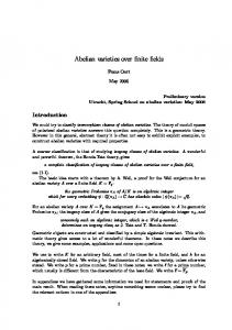
Fig. 1: (a) The ten rings of S2VD; (b) Cell x and its neighbor y cells; (c) The counterexample

Quantifier Elimination over Finite Fields Using Gr¨ obner Bases

153

The S2VD Model The model consists of a hexagonal grid of cells. Each hexagon represents a cell, and each cell has six neighbors. There are four possible colors for each cell. A green cell is infected with (the good) Virus G, and a red cell is infected with (the bad) Virus R. When the two viruses meet in one cell, Virus G captures Virus R and the cell becomes yellow. A cell not infected by any virus is white. The dynamics of the system is determined by the interaction of the viruses. There are ten rings of cells in the model, with a total of 331 cells (Figure 1(a)). In the initial configuration, the cells in Ring 4 to 10 are set to white, and the cells in Ring 1 to 3 can start with arbitrary colors. The aim is to have a controller that satisfies the following safety property: The cells in the outermost ring are either green or white at all times. The proposed controller detects if any cell has been infected by Virus R, and injects cells that are “one or two rings away” from it with Virus G. The injected Virus G is used to block the further expansion of Virus R. Formally, the model is a polynomial system over the finite field F4 = {0, 1, a, a+ 1}, with each element representing one color: (0, green), (1, red), (a, white), (a + 1, yellow). The dynamics is given by the function f : F4331 → F4331 . For each cell x, its dynamics fx is determined by the color of its six neighbors y1 , ..., y6 , specified by the nonlinear polynomial fx =df γ22 + γ2 γ13 + a2 (γ13 + γ12 + γ1 ), where P6 P γ1 = i=1 yi and γ2 = i6=j yi yj . The designed controller is specified by another function g : F4331 → F4331 : For each cell x, with y1 , ..., y18 representing the cells Q18 in the two rings surrounding it, we define gx =df i=1 (1 − yi )3 . More details can be found in [11]. Applying Quantifier Elimination We first try checking whether the safety property itself forms an inductive invariant of the system (which is a strong sufficient check). To this end, we check whether the controlled dynamics of the system remain inside the invariant on the boundary (Ring 10) of the system. Let x be a cell in Ring 10 and y = (y1 , ..., y18 ) be the cells in its immediate two rings. We assume the cells outside Ring 10 (y8 , ..., y12 , y2 , y3 ) are white. See Figure 1(b) for the coding of the cells. We need to decide the formula: ∀x((∃y((

12 ^

(yi = a) ∧ y2 = a ∧ y3 = a) ∧ Safe(y) ∧ x = Fx (y))) → x(x − a) = 0) (3) | {z } {z } “green/white”

i=8

|

where (writing γ1 =

ϕ1

P6

i=1

yi , γ2 =

P

i6=j∈{1,...,6}

yi yj )

Safe(y) =df (y1 (y1 − a) = 0 ∧ y4 (y4 − a) = 0 ∧ y7 (y7 − a) = 0 ∧ y13 (y13 − a) = 0) Fx (y) =df (γ22 + γ2 γ13 + a2 (γ13 + γ12 + γ1 )) · (

18 Y

(1 − yi ))3

i=1

After quantifier elimination, Formula (3) turns out to be false. In fact, we obtained Jϕ1 K = Jx4 − x = 0K. Therefore, the safety property itself is not an inductive invariant of the system. We realized that there is an easy counterexample

154

Sicun Gao, Andr´e Platzer, and Edmund M. Clarke

of safety of the proposed controller design: Since the controller is only effective when red cells occur, it does not prevent the yellow cells to expand in all the cells. Although this is already a bug of the system, it may not conflict with the authors’ original goal of controlling the red cells. However, a more serious bug is found by solving the following formula:

|

18 ^

yi (yi − a)(yi − a2 ) = 0) ∧ x = Fx (y)) → ¬(x = 1) ) | {z } i=1 {z } “not red”

∀x((∃y(

(4)

ϕ2

Formula (4) expresses the desirable property that when none of the neighbor cells of x is red, x never becomes red. However, we found again that Jϕ2 K = Jx4 − x = 0K, which means in this scenario the x cell can still turn red. Thus, the formal model is inconsistent with the informal specification of the system, which says that non-red cells can never interact to generate red cells. In fact, the authors mentioned that the dynamics Fx is not verified because of the combinatorial explosion. Finally, to give a counterexample of the design, we solve the formula ϕ3 =df ∃y∃x.(x = 1 ∧

6 ^

yi (yi − a)(yi − a2 ) = 0 ∧ x = Fx (y))

(5)

i=1

The formula checks whether there exists a configuration of y1 , ..., y6 which are all non-red, such that x becomes red. ϕ3 evaluates to true. Further, we obtain x = 1, y = (a, a, a, 0, 0, 0) as a witness assignment for ϕ3 . This serves as the counterexample (see Figure 1(c)). This example shows how our quantifier elimination procedure provides a practical way of verifying and debugging systems over finite fields that were previously not amenable to existing formal methods and cannot be approached by exhaustive enumeration.

7

Conclusion

In this paper, we gave a quantifier elimination algorithm for the first-order theory over finite fields based on the Nullstellensatz over finite fields and Gr¨obner basis computation. We exploited special properties of finite fields and showed the correspondence between elimination of quantifiers, projection of varieties, and computing elimination ideals. We also generalized the Tseitin transformation from Boolean formulas to formulas over finite fields using ideal operations. The complexity of our algorithm depends on the complexity of Gr¨obner basis computation. In an application of the algorithm, we successfully found bugs in a biological controller design, where the original authors expressed that no verification methods were able to handle the system. In future work, we expect to use the algorithm to formally analyze more systems with finite field arithmetic. The scalability of the method will benefit from further optimizations on Gr¨obner basis computation over finite fields. It is also interesting to combine Gr¨obner basis methods and other efficient Boolean methods (SAT and QBF solving). See [9] for a discussion on how the two methods are complementary to each other.

Quantifier Elimination over Finite Fields Using Gr¨ obner Bases

155

Acknowledgement The authors are grateful for many important comments from Jeremy Avigad, Helmut Veith, Paolo Zuliani, and the anonymous reviewers.

References 1. 2. 3. 4. 5.

6. 7. 8. 9. 10. 11.

12.

13. 14. 15. 16. 17.

The SAGE Computer Algebra system, http://sagemath.org The Singular Computer Algebra system, http://www.singular.uni-kl.de/ Becker, T., Weispfenning, V.: Gr¨ obner Bases. Springer, (1998) Le Borgne, M., Benveniste, A., Le Guernic, P.: Polynomial dynamical systems over finite fields. In: Algebraic Computing in Control, Vol. 165, Springer, (1991) Marchand, H., Le Borgne, M.: On the Optimal Control of Polynomial Dynamical Systems over Z/pZ. In: 4th International Workshop on Discrete Event Systems, pp. 385–390 (1998) Buchberger, B.: A Theoretical Basis for the Reduction of Polynomials to Canonical Forms. In: ACM SIGSAM Bulletin, 10(3), pp.19-29, (1976) Cox, D., Little, J., O’Shea, D.: Ideals, Varieties, and Algorithms. Springer (1997) Cox, D., Little, J., O’Shea, D.: Using Algebraic Geometry. Springer (2005) Gao, S.: Counting Zeroes over Finite Fields with Gr¨ obner Bases. Master Thesis, Carnegie Mellon University (2009) Germundsson, R.: Basic results on ideals and varieties in Finite Fields. Technical Report LiTH-ISY-I-1259, Linkoping University, S-581 83 (1991) Jarrah, A., Vastani, H., Duca, K., and Laubenbacher, R.: An Optimal Control Problem for in vitro Virus Vompetition. In: 43rd IEEE Conference on Decision and Control (2004) Jarrah, A.S., Laubenbacher, R., Stigler, B., and Stillman, M.: Reverse-engineering of polynomial dynamical systems. In: Advances in Applied Mathematics, vol. 39, pp 477–489 (2007) Lakshman, Y.N.: On the Complexity of Computing a Gr¨ obner Casis for the Radical of a Zero-dimensional Ideal. In STOC ’90, pp 555–563, New York, NY, USA, (1990) Lang, S.: Algebra, 3rd Edition. Springer (2005) Marker, D.: Model theory. Springer (2002) Smith, E.W., Dill, D.L.: Automatic Formal Verification of Block Cipher Implementations. In: FMCAD, pp. 1–7 (2008) Tran, Q.N.: Gr¨ obner Bases Computation in Boolean Rings is PSPACE. In: International Journal of Applied Mathematics and Computer Sciences, vol. 5, No. 2, (2009)

156

Sicun Gao, Andr´e Platzer, and Edmund M. Clarke

Appendix: Omitted Proofs Proof of Lemma 2.1 This is a consequence of the Seidenberg’s Lemma (Lemma 8.13 in [3]). It can also be directly proved as follows. p Proof. We need to show J + hxq1 − x1 , ..., xqn − xn i = J + hxq1 − x1 , ..., xqn − xn i. Since by definition, any ideal is contained in its radical, we only need to prove q J + hxq1 − x1 , ..., xqn − xn i ⊆ J + hxq1 − x1 , ..., xqn − xn i. 1 , ..., xn ]. Consider an arbitrary polynomial f in the ideal p Let Rq denote Fq [x q J + hx1 − x1 , ..., xn − xn i. By definition, for some integer s, f s ∈ J + hxq1 − x1 , ..., xqn − xn i. Let [f ] and [J] be the images of, respectively, f and J, in R/hxq1 − x1 , ..., xqn − xn i under the canonical homomorphism from R to R/hxq1 − x1 , ..., xqn − xn i. For brevity we write S = hxq1 − x1 , ..., xqn − xn i. Now we have [f ]s ∈ [J], and we further need [f ] ∈ [J]. We prove, by induction on the structure of polynomials, that for any [g] ∈ R/S, [g]q = [g].

– If [g] = cxa1 1 · · · xann + S (c ∈ Fq , ai ∈ N ), then [g]q = (cxa1 1 · · · xann + S)q = (cxa1 1 · · · xann )q + S = cxa1 1 · · · xann + S = [g]. – If [g] = [h1 ] + [h2 ], by inductive hypothesis, [h1 ]q = [h1 ], [h2 ]q = [h2 ], and, since any element divisible by p is zero in Fq (q = pr ), then [g]q = ([h1 ] + [h2 ])q =

q   X q i=0

i

[h1 ]i [h2 ]q−i = [h1 ]q + [h2 ]q = [h1 ] + [h2 ] = [g]

Hence [g]q = [g] for any [g] ∈ R/S, without loss of generality we can assume s < q in [f ]s . Then, since [f ]s ∈ [J], [f ] = [f ]q = [f ]s · [f ]q−s ∈ [J]. t u Proof of Lemma 3.1 Proof. Let V a ∈ Fqn+m be an assignment vector for (x, y). r If a ∈ J i=1 fi = 0K, then fV1 (a) = · · · = fr (a) = 0 and a ∈V V (hf1 , ..., fk i). r r u If a ∈ V (hf1 , ..., fr i), then i=1 fi (a) = 0 is true and a ∈ J i=1 fi = 0K. t Proof of Lemma 3.2 Proof. We show set inclusion in both directions. – For any b ∈ J∃xϕ(x; y)K, by definition, there exists a ∈ Fqn such that (a, b) satisfies ϕ(x; y). Therefore, (a, b) ∈ Jϕ(x; y)K, and b ∈ πn (Jϕ(x; y)K). – For any b ∈ πn (Jϕ(x; y)K), there exists a ∈ Fqn such that (a, b) ∈ Jϕ(x; y)K. By definition, b ∈ J∃xϕ(x; y)K. t u

Quantifier Elimination over Finite Fields Using Gr¨ obner Bases

157

Proof of Lemma 3.3 V V Proof. We have J i∈Ax (xqi − xi = 0) ∧ i∈Ay (yiq − yi = 0)K = J>K, which follows from Proposition 2.1. t u Proof of Lemma 4.1 Proof. Let ϕ[ψ1 /ψ2 ] denote substitution of ψ1 in ϕ by ψ2 . Suppose the negative atomic formulas in ϕ are f1 6= 0, ..., fk 6= 0. We introduce a new variable z1 , and substitute f1 6= 0 by p · z1 = 1. Since the field Fq does not have zero divisors, all the solutions for Jf1 6= 0K = J∃z1 (p · z1 = 1)K (the Rabinowitsch trick). Iterating the procedure, we can use k new variables z1 , ..., zk so that: JϕK = Jϕ[f1 6= 0/(∃z1 .(p · z1 − 1 = 0))] · · · [fk 6= 0/(∃zk .(p · zk − 1 = 0))]K

Since the result formula contains no more negations and the zi s are new variables, it can be put into prenex form ∃z.(ϕ[f1 6= 0/(p·z1 −1 = 0)] · · · [fk 6= 0/(p·zk −1 = 0)]). t u Proof of Lemma 4.2 Proof. Jψ1 ∨ ψ2 K = V (J1 ) ∪ V (J2 ) follows from the definition of realization. We only need to show the second equality. Let a = (a1 , ..., an ) ∈ Fqn be a point. - Suppose a ∈ V (J1 ) ∪ V (J2 ). If a ∈ V (J1 ), then (1, a1 , ..., an ) ∈ V (x0 J1 + (1 − x0 )J2 ). If a ∈ V (J2 ), then h0, a1 , ..., an i ∈ V (x0 J1 + (1 − x0 )J2 ). In both cases, a ∈ π0 (V (x0 J1 + (1 − x0 )J2 )). - Suppose a ∈ π0 (V (x0 J1 + (1 − x0 )J2 )). There exists a0 ∈ Fq such that (a0 , a1 , ..., an ) ∈ V (x0 J1 + (1 − x0 )J2 ). If a0 6∈ {0, 1}, then all the polynomials in J1 and J2 need to vanish on a; if a0 = 1 then J1 vanishes on a; if a0 = 0 then J2 vanishes on a. In all cases, a ∈ V (J1 ) ∪ V (J2 ). t u Proof of Theorem 5.1 Proof. We only need to show the intermediate formulas obtained in Step 1-3 are always equivalent to the original formula ϕ. In Step 1, the formula is flattened with ideal operations, which preserve the realization of the formula Vr as proved in Theorem 4.1. In Step 2, we have (by Theorem 3.2) J∃x ∃t∃s( m i=1 (fi = 0))K = Vu J i=1 (gi = 0)K. Hence the formula obtained in Step 2 is equivalent to ϕ. In Step 3, the substitution preserves realization of the formula because u ^

J

i=1

∀xm−1 (gi = 0)K = J

u ^

(¬∃xm−1 (¬gi = 0))K = J(

i=1

vi u _ ^ ( hij 6= 0))K,

i=1 j=1

where the second equality is guaranteed by Theorem 3.2 again. The loop terminates either at the end of Step 2 or Step 3. Hence the output quantifier-free formula ψ is always in conjunctive normal form, which contains only variables y, and is equivalent to the original formula ϕ. t u