Front. Energy 2015, 9(1): 115–124 DOI 10.1007/s11708-015-0348-8
RESEARCH ARTICLE
Shangguang YANG, Chunlan WANG, Kevin LO, Mark WANG, Lin LIU
Quantifying and mapping spatial variability of Shanghai household carbon footprints
© Higher Education Press and Springer-Verlag Berlin Heidelberg 2015
Abstract Understanding the spatial variability of household carbon emissions is necessary for formulating sustainable and low-carbon energy policy. However, data on household carbon emissions is limited in China, the world’s largest greenhouse gases emitter. This study quantifies and maps household carbon emissions in Shanghai using a city-wide household survey. The findings reveal substantial spatial variability in household carbon emissions, especially in transport-related emissions. Low emission clusters are founded in Hongkou, Xuhui, Luwan, Jinshan, and Fengxian. High emission clusters are located in Jiading and Pudong. Overall, the spatial pattern of household carbon emissions in Shanghai is donut-shaped: lowest in the urban core, increasing in the surrounding suburban areas, and declining again in the urban fringe and rural regions. The household emissions are correlated with a number of housing and socioeconomic factors, including car ownership, type of dwelling, size of dwelling, age of dwelling, and income. The findings underscore the importance of a localized approach to low-carbon policymaking and implementation. Keywords household carbon emissions, spatial variability, energy policy, Shanghai, China
Received June 26, 2014; accepted October 24, 2014 Shangguang YANG, Lin LIU Institute of Economic Development, East China University of Science and Technology, Shanghai 200237, China Chunlan WANG School of Social Development, East China Normal University, Shanghai 200062, China
✉
Kevin LO ( ) Department of Geography, Hong Kong Baptist University, Hong Kong, China E-mail:
[email protected] Mark WANG School of Geography, University of Melbourne, VIC 3010, Australia
1
Introduction
Climate change is one of the most significant global energy challenges and households are increasingly seen as important contributors to the problem [1, 2]. Households directly and indirectly produce carbon emissions from various types of activities, including energy use at home (e.g., space heating, air conditioning, lighting, and cooking), transportation (e.g., personal vehicle and public transit use), and the consumption of goods and services (i.e., embodied emissions). Although Chinese households contribute a relatively small proportion of national carbon emissions, absolute and relative household emissions have been rapidly increasingly due to rapid urbanisation and increasing wealth which drive the consumption of energyintensive goods and services [3]. Two examples suffice to illustrate this trend. First, the penetration rate of air conditioning systems in China’s urban households grew from less than 1% in 1990 to 62% in 2003 [4]. Second, private vehicle ownership grew equally rapidly, from 0.71 vehicles to 54 vehicles per thousand people from 1990 to 2011 [5]. Therefore, an analysis of China’s household carbon footprints is one of the most important topics in energy research. Much past and recent works on China’s household carbon emissions use national-level statistics to conduct cross-region comparison with respect to household carbon footprints. For example, Zheng et al. [6] examined 74 Chinese cities and found the households in the dirtiest cities (Daqing, Mudanjiang, and Beijing) emitted three to four times as much carbon as the households in the cleanest cities (Huai’an, Suqian, and Haikou). According to the authors, the intercity difference can largely be explained by the presence of carbon-intensive centralised heating in northern Chinese cities. Liu et al. [3] used national-level input-output data to estimate China’s carbon emissions from rural and urban households and found a significant upward trend for both cases from 1992 to 2007. While these findings are important, emission inventories at the national level cannot shed light on the spatial variability of
116
Front. Energy 2015, 9(1): 115–124
household emissions within a locality. Studies conducted outside China have illuminated the magnitude of this spatial variability and the contributing spatial factors such as urban form, availability of public transport, quality and quantity of the housing stock, and rural-urban separation [7, 8]. To formulate sustainable local energy policy and avoid dangerous climate change, policymakers and urban planners need to understand the spatial variability of household carbon footprints. This paper presents a pioneering study of the spatial distribution of household carbon emissions in Shanghai, one of China’s most important economic centers. The study has been guided by three questions: ① What is the spatial distribution of household carbon emissions in Shanghai? ② What are the most important spatial and socio-economic factors influencing household carbon emissions in Shanghai? ③ What insights can be gained for guiding future urban policy and planning? Using a quantitative survey approach and applying geographic information systems (GIS) and statistical analysis, this study maps Shanghai household carbon emissions to highlight both spatial and non-spatial properties. The study is concerned with household carbon emissions from direct sources only and primarily tracks emissions associated with energy use at home and transport. Indirect or embodied emissions are not considered because they are not directly relevant to the main objective of providing local governments with relevant policy recommendations on household emissions reduction. From a local government perspective, reducing embodied emissions is difficult, if not impossible, in a global trading system [9, 10]. This paper proceeds in five sections following this introduction. The first section surveys the recent literature on the determinants of household carbon emissions. The second section introduces the research method. The third section thematically maps Shanghai household carbon emissions and discusses some observations about the spatial characteristics. Results from the spatial autocorrelation analysis are also presented in this section. The fourth section identifies the significant housing and socioeconomic factors of household emissions as well as the relationship between different factors using correlation analysis. Finally, the fifth section summarizes the findings and discusses relevant policy implications.
2 Factors contributing to spatial variability of household carbon emissions The paper provides convincing evidence that there is significant spatial variation in household energy consumption and carbon emissions within a city’s boundary. A number of spatial, housing, and socioeconomic factors have been found to contribute to the difference in household emissions. Turning first to spatial factors, the location of household
relative to the city center is a strong predictor of household carbon emissions. A significant number of empirical studies have found that transport-related emissions increase with distance from the urban core [1, 2, 11, 12]. This is primarily due to the fact that suburban households often have less access to public transit and a greater reliance on automobiles. Furthermore, because most cities have a high concentration of workplaces, shopping malls, schools, and leisure facilities in the urban center, suburban households often need to make longer and more frequent trips than their inner-city counterparts to access these facilities. The policy implication of such findings is an emphasis on compact cities (as opposed to sprawling cities) as a low-carbon, energy-efficient urban development objective. However, Wilson et al. [13] found that in the Canadian city of Halifax, households from the suburbs generate similar amounts of transportation emissions to those in the inner city because there are an abundance of jobs and recreational opportunities in the suburbs. Their study highlights how spatial dynamics driving household carbon emissions are complex and are to some extent specific to individual cities. The spatial variability of household carbon emissions is also dependent on a number of housing factors. For example, energy consumption from space heating is dependent on the dwelling size and type, building insulation levels, and heating system efficiency [9, 10]. The age of the dwelling is also an important factor as older buildings are usually less energy efficient [14]. Others, however, have suggested that newer buildings, especially high-rise buildings, are less energy efficient [15]. Furthermore, the type of resident tenure is a strong predictor of investment in energy conservation measures and therefore household carbon emissions from energy use at home. In general, rental properties have a low adoption rate of energy efficiency measures due to a mismatch between the party paying for the energy efficiency improvements (the landlord) and the party receiving the benefits (the tenant) [16]. A number of policy responses have been developed to address this problem, most notably the Chinese government’s ambitious program to provide governmentfunded energy conservation retrofits to existing residential buildings [17]. Housing factors often also have a spatial dimension. For example, the city center’s housing stock is typically older and therefore less energy efficient than those in the surrounding suburbs [13]. Urban cores’ high housing densities are also associated with lower rates of residential renewable energy installations [18]. Further, city center households may need to use more energy on cooling because of the urban heat island effect due to high density and the lack of vegetation; however, this effect may be reversed when heating is required in winter. Finally, a number of socioeconomic factors are found to be significant predictors of household carbon emissions. Carbon emissions are not just positively correlated with household size, but also with household members’ income
Shangguang YANG et al. Spatial variability of Shanghai household carbon footprints
and education levels [19, 20]. Households with higher incomes are likely to spend more on both direct and indirect energy consumption and live in a larger dwelling. Zheng et al. [6] found that richer cities have significantly higher household carbon emissions as well. Education is also positively correlated with household emissions, possibly because of its association with higher income levels [21]. Similar to housing factors, socioeconomic factors also have a spatial dimension in that cities are often segregated socioeconomically. For example, Druckman and Jackson [9] found that households in the most affluent suburbs are responsible for 64% more CO2 than households in the least affluent suburbs.
3
Data and methods
3.1
Study area
Shanghai is situated on the east coast of China at 31.12°N latitude and 121.30°E longitude. It is one of the four provincial-level cities and the most populous Chinese city.1) According to the last census conducted in 2010, Shanghai has a population of 23 million people. Shanghai’s administrative boundary covers an area of 6340.5 km2, extending approximately 100 km inward from the coast to the inland border with Jiangsu province. The Huangpu River divides Shanghai’s urban core into two main areas: Puxi, the historic city center of Shanghai, and Pudong, a former rural locality transformed in less than two decades into the city’s most modern and developed district. Despite its image as an urban metropolis, Shanghai still has patches of rural landscapes, most notably along the eastern and southern rim of the city, as well as on Chongming Island in the Yangtze River estuary. While Shanghai’s transformation into one of the world’s
117
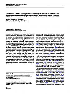
leading global cities has been impressive, its increasing prosperity has led to concerns regarding environmental impact and climate change. From 1980 to 2011, annual energy consumption in Shanghai increased by more than 5fold, from 21.3 million tons coal equivalent (tce) in 1980 to 109.4 million tce in 2011 (Fig. 1). The calculation by Li et al. [22] demonstrated that Shanghai’s energy-related greenhouse gas emissions increased from 109 million tons of CO2 in 1995 to 184 million tons of CO2 in 2006, with projected emissions rising to 630 million tons of CO2 by 2020 under a business-as-usual scenario or 330 million tons of CO2 under a best policy scenario. Wang et al. [23] found that the city’s total carbon emissions from 2000 to 2008 increased from 136 to 200 teragrams of CO2 equivalent. In 2008, Shanghai’s per capita emissions reached 14.03 tons of CO2, which were higher than both the world average and the average in China. Both studies found that residential and transportation emissions significantly contribute to emissions increases as Shanghai transforms into a post-industrial city. 3.2
Data collection
Household surveys are typically conducted through mailed survey questionnaires or telephone interviews. However, these methods are often plagued by low response rates, which impact the generalisability of findings. To address this problem, we chose to administer face-to-face surveys. This data collection approach also allowed us to clarify questions immediately, thereby enhancing the completion rate and the validity of the findings. Additionally, face-toface contact allows for more complicated selection methods and provides better coverage of households living in different districts. The questionnaires consisted of four sections. Section one asked for information regarding the residential dwelling and the neighborhood, such as the
Fig. 1 Energy consumption in Shanghai (1980–2011) (Source: Shanghai Statistical Yearbook)
1) Provincial-level cities are at the same administrative level as provinces and therefore have more power and enjoy more support from the central government compared to other Chinese cities.
118
Front. Energy 2015, 9(1): 115–124
size, age, and type of dwelling, the name of the residing neighborhood, and the availability of commercial and public facilities in close proximity to the dwelling. Section two enquires about transport patterns, and the data are used to calculate transport-related carbon emissions. The main questions include how far and how often household members need to travel for work/school and for leisure, the means of transportation, and the average cost of petrol if the household owns a car. Section three asks about energy use at home. The main questions are how much electricity is used per month in different seasons, the availability of a centralised heating system, and how much coal gas, liquefied petroleum gas, and natural gas are consumed per month. Finally, section four collects household information, including the number of household members, household income, and educational achievements. Between June and September 2012, a team of interviewers visited different parts of Shanghai and a diverse set of locations, including residential areas, metro stations, bus stations, shops, parks, and local community centers. The interviewers distributed the questionnaire survey to 1200 respondents, and a total of 1054 (88%) valid questionnaires were received. A sectoral analysis of the responses confirmed that they reflect the underlying character of the population of Shanghai at-large (Table 1). Table 1 Comparison of sample and census population characteristics Age
Household size
Education
Sample/%
Shanghai census (2010)/%
0–19
13.72
13.48
20–29
24.66
22.55
30–44
27.86
25.75
45–59
28.71
23.14
60 and up
5.05
15.07
1 person
10.63
19.89
2 people
14.46
33.99
3 people
52.37
30.89
4 people
14.49
8.88
5 people or more
8.05
6.35
Junior high school
15.55
53.95
Senior high school
24.73
22.52
Vocational college
19.39
10.35
Undergraduate
30.58
11.21
Postgraduate
9.75
1.97
4 Spatialvariation of household emissions in Shanghai 4.1
Descriptive analysis
Our results demonstrate that the average annual household carbon footprint in Shanghai is 3206.15 kgCO2/a, with
59% coming from energy use at home (1902.72 kgCO2/a) and 41% from transport-related activities (1303.43 kgCO2/a). The emissions levels are substantially higher than the 1796 kgCO2/a estimated by Zheng et al. [6]. This is likely due to the difference in time; Zheng et al. [6] used 2006 data whereas our survey was conducted much more recently. Despite the significant rise in emissions, households in Shanghai remain substantially less carbon intensive than those in the United States. On average, households in the greenest American cities (e.g., San Francisco and San Diego) still emit approximately eight times more than households in Shanghai [24]. Figure 2 illustrates the average annual household emissions across 17 Shanghai districts. The spatial variation in carbon emissions across households is substantial even at this aggregated level. The lowest levels of emissions were recorded in the Luwan district with 2095 kgCO2/a and the Fengxian district with 2099 kgCO2/a. Luwan is an inner city district at the heart of the metropolitan area that has good access to public transit, jobs, and amenities; Fengxian, on the other hand, is a rural district with poor access to transport and amenities and a high percentage of rural populations. The highest levels of emissions were recorded in the Jiading district with 4563 kgCO2/a, the Baoshan district with 3493 kgCO2/a, and the Pudong district with 3365 kgCO2/a. These high-emission districts are all suburban residential districts dotted with luxurious apartment buildings and a car-dependent lifestyle, which is reflected in their high transport-related emissions levels. For the majority of districts, the average annual household emissions ranged from 2800 kgCO2/a to 3500 kgCO2/a. It may also be noted that while in most cases, energy use at home is the dominant type of household emissions, the variability is much greater in transport-related emissions. Transport-related emissions range from the lowest value of 204 kgCO2/a in the Luwan district to the highest value of 2594 kgCO2/a in the Jiading district. In contrast, emissions from energy use at home range from the lowest value of 1549 kgCO2/a in the Fengxian district to the highest value of 2211 kgCO2/a in Hongkou. This result demonstrates that spatial variation in household carbon emissions is mainly due to differences in transport-related emissions rather than energy use at home. 4.2
Thematic mapping
To better visualize the spatial variation of household carbon emissions in Shanghai, the survey data were fed into a GIS platform to produce thematic maps. Figure 3 plots the household carbon emissions data from energy use at home only. The map confirms the previous finding that the difference in emissions from energy use at home across households is not significant, with most households producing between 1000 kgCO 2 and 2000 kgCO 2 annually. Households with the highest levels of emissions
Shangguang YANG et al. Spatial variability of Shanghai household carbon footprints
119
Fig. 2 Household carbon emissions in different Shanghai districts
Fig. 3 The spatial pattern of Shanghai household carbon emissions from energy use at home
from energy use at home are located in the city center and the surrounding suburban areas. Households from the rural areas tend to have lower levels of emissions. This finding thus illustrates the rural-urban divide of energy use at home in Shanghai; urban energy consumption is much greater than rural consumption.
Figure 4 illustrates the spatial distribution of Shanghai household carbon emissions from transport-related activities only. As expected, variation in household emissions from transport is more significant than that associated with energy use at home. The difference between the highest and lowest emissions levels is more than 10-fold. The
120
Front. Energy 2015, 9(1): 115–124
Fig. 4 The spatial pattern of Shanghai household carbon emissions from transport
spatial pattern is also very different from energy use at home. Households with low transport emissions are mainly in the city center and the rural districts, suggesting that households in these districts have fewer travel needs than those located in the suburbs. On the other hand, suburban households have longer and more frequent travel needs, as well as a higher car ownership rate. The fact that suburban households have the highest transport emissions indicates that the suburban districts of Shanghai are home to large residential developments for commuters to the central city. Figure 5 shows the spatial distribution of Shanghai household carbon emissions from both energy use at home and transport. The spatial pattern from both emission types is donut-shaped: emissions are the lowest in the urban core, increase in the surrounding suburban areas, and decline again in the urban fringe and rural regions. Suburban districts, in particular in Pudong, Hongkou, Baoshan, and Jiading, have the highest concentration of households with high carbon emissions levels. In contrast, the households in the central districts (e.g., Jingan, Luwan, Zhabei, and Huangpu) and the rural districts (e.g., Jinshan and Fengxian) tend to have low carbon emissions. This spatial pattern can be almost entirely attributed to transportationrelated emissions. The effect of energy use at home on overall household emissions’ spatial variability is not significant. 4.3
Global spatial autocorrelation
Global spatial autocorrelation (i.e., Moran’s I index) is a
measure of the overall clustering of the data. A positive value indicates spatial clustering of similar values and a negative value, clustering of dissimilar values. The household emissions data were analyzed using Moran’s I index to determine the extent of significant spatial clustering in household carbon emissions. The Moran’s I index for our data are 0.005212, which indicates the presence of clustering of households with similar carbon emissions values. Statistical significance of the Moran’s I index can be assessed based on the p-value and the z-score. The p-value is a probability score indicating the significance of the index. When the p-value is small, the correlation is unlikely to occur by chance. The z-score is a measurement of standard deviation and is also used to indicate the index’s significance. A high or low z-score also indicates that the result is unlikely to be random. Our analysis found a p-value of 0.088 and a z-score of 1.71, indicating that at a 90% confidence level, the clustering result is statistically significant and did not occur by chance. 4.4
Local spatial autocorrelation
To measure local spatial association and to identify statistically significant clusters, we calculated the GetisOrdGi* statistic to generate a map illustrating hot and cold spots for household carbon emissions. The Getis-OrdGi* statistic compares the local mean to the global mean and produces a z-score for each area indicating whether the differences between the means are statistically significant.
Shangguang YANG et al. Spatial variability of Shanghai household carbon footprints
121
Fig. 5 The spatial distribution of Shanghai household carbon emissions from both energy use at home and transport
A statistically significant positive z-score indicates a hot spot (i.e., a local clustering of above-average values) whereas a statically significant negative z-score indicates a cold spot (i.e., a local clustering of below-average values). To make the results easier to visualize, we divided the zscore into seven categories. The results are shown in Fig. 6. The distribution of hotspots (red) and cold spots (blue) is
distinctive and reflects the donut-shaped pattern identified previously. Low emission clusters are concentrated in Hongkou, Xuhui, and Luwan. These central districts are high-density residential areas with well-established public transport; they have a wide array of commercial and community facilities nearby. Low emission clusters can also be found in the rural areas of Jinshan and Fengxian.
Fig. 6 Local spatial association of household carbon emissions in Shanghai
122
Front. Energy 2015, 9(1): 115–124
Most high emission clusters are located in Jiangqiao in the Jiading district and Huinan in the Pudong district. In these suburban areas, rapidly growing residential developments outpace investment in commercial facilities, public facilities, and transportation, so daily commuting needs are high. 4.5
Correlation analysis
Our survey also collected information about socioeconomic and housing factors, which can be used to further shed light on the causes to spatial variability of household carbon emissions in Shanghai. In total, there are 3 independent variables and 16 dependent variables (Table 2). Table 2 Dependent and independent variables used in regression and correlation analysis Variable symbol Y1
Meaning Total household emissions
Y2
Household emissions from transport
Y3
Household emissions from energy use at home
X1
Home tenure (rental or owner-occupation)
X2
Nature of dwelling (commodity housing, affordable housing, or public housing)
X3
Size of dwelling
X4
Household registration
X5
Age of dwelling
X6
Type of dwelling (low-rise building, high-rise building, detached house, semi-detached house, or row house
X7
Car ownership
X8
Household size
X9
Age of the first household member
X10
Age of the second household member
X11
Age of the third household member
X12
Education of the first household member
X13
Education of the second household member
X14
Employment of the first household member
X15
Employment of the second household member
X16
Income
We conducted three types of correlation analysis: correlation between dependent variables, correlation between independent variables, and correlation between dependent and independent variables. Turning first to the correlation between dependent variables, we found that the Pearson correlation coefficient between household emissions from transport and from energy use at home is 0 (significance level = 0.01), which indicates no linear relationship between the two variables. Households with high emissions levels from energy use at home do not
necessarily generate more emissions from transport. This suggests there are different factors influencing the two types of household emissions. In computing the correlation between the five housingrelated independent variables (X1, X2, X3, X5, and X6), we found positive correlations between X3 (size of dwelling) and X6 (type of dwelling), and between X5 (age of dwelling) and X6 (type of dwelling). The correlation coefficients are 0.350 and 0.306, respectively (significance level = 0.01), which indicates that some of the housing variables are interrelated. We also analyzed the correlation between five socioeconomic independent variables (X12, X13, X14, X15, and X16). The correlation between the household members’ education levels (X12 and X13) is significant (correlation coefficient = 0.672, significance level = 0.01). The correlations between education and employment, between income and education, and between income and employment were also significant. This suggests that there is a relationship between the various socioeconomic variables. In assessing the correlation between dependent and independent variables, we found that total household emissions where correlated with car ownership (X7), type of dwelling (X6), size of dwelling (X3), income (X16), and age of dwelling (X5) (Table 3). The correlation coefficients are, respectively, –0.331, 0.182, 0.145, 0.120, and 0.086. Car ownership is the most significant correlate to household emissions, which suggests that households that have cars use them regularly, resulting in higher emissions. The type and size of dwelling are also significantly correlated with household emissions from energy use at home and from transport. This correlation may occur because these Table 3 Results of correlation analysis between dependent and independent variables Variable
Pearson's correlation coefficient Significance (two-tailed)
X1
–0.390
0.207
X2
0.009
0.775
X3
0.145
0.000
X4
–0.072
0.019
X5
0.086
0.006
X6
0.182
0.000
X7
–0.331
0.000
X8
0.181
0.000
X9
–0.007
0.817
X10
0.007
0.839
X11
–0.020
0.588
X12
0.025
0.426
X13
0.027
0.421
X14
–0.033
0.293
X15
–0.035
0.291
X16
0.120
0.000
Shangguang YANG et al. Spatial variability of Shanghai household carbon footprints
two factors not only influence energy use at home but also reflect the household’s location, which is a key spatial determinant of household emissions from transport. Finally, income and size of household positively correlate with household emissions. Interestingly, employment, age, and education are not strongly correlated with household emissions.
5
Conclusions and discussion
This study’s findings suggest three key conclusions. First, Shanghai’s household carbon emissions are non-homogeneous, with low-carbon households concentrated in the urban center and rural regions and high-carbon households in suburban areas. In other words, the spatial pattern of household carbon emissions can be described as donutshaped. However, this should not be interpreted as a confirmation that the inner-city is more sustainable than the suburbs. Rather, both areas have different challenges that require policy attention. In general, inner-city households have higher emissions from energy use at home because of the type and age of dwellings commonly found there. Second, household emissions are correlated with a number of housing and socioeconomic factors, including car ownership, type of dwelling, size of dwelling, age of dwelling, and income. Lastly, there is no linear relationship between household emissions from energy use at home and from transport, indicating that different factors are involved in determining the two types of household emissions. The distance between residential areas and employment opportunities, the availability of facilities and amenities, and the quality of public transport and car ownership are the key factors influencing transport-related household emissions; the age, type, and size of dwellings affect emissions from energy use at home. In sum, examining Shanghai’s household emissions reveals substantial spatial variability and indicates the need for policy solutions that address this variability. Therefore, the key policy implication of this study is to advocate for a more localized approach to low-carbon urban governance. Metropolises are complex systems with significant spatial variations in household carbon emissions. Therefore, an approach that is sensitive to local (i.e., sub-city, neighborhood, or residential area) circumstances could provide more precise and effective interventions promoting household energy conservation. In Shanghai, the highest levels of household transport emissions stem from the sprawling suburban residential areas, reflecting the negative environmental impact of urban sprawl and a monocentric urban system. Public transit investment and improvement, such as rapid bus transit and rail-based mass transit connecting to the city center, should be prioritised in these areas. At the same time, the government should look into improving the provision of local facilities and economic opportunities to reduce the need for long-distance com-
123
muting and other travel. In contrast, the inner-city districts have the highest levels of household emissions from energy use at home, which is associated with high income levels and with the number of old buildings that lack or have insufficient insulation. The government should focus on retrofitting old buildings with insulation, promoting the use of energy efficient appliances, and encouraging the adoption of renewable energy solutions such as solar water heaters and photovoltaic systems. For rural areas, which currently have a low level of both household emissions types, policy challenges focus on balancing the need to improve living standards and the need to control emissions. In this context, the promotion of energy efficient appliances and renewable energy technologies is highly recommended. Acknowledgements The project was funded by the National Social Science Foundation (No. 11CRK005), the Ministry of Education Humanities and Social Science Foundation (No. 11YJA630176), the Shanghai Municipal Soft Science Foundation, the Australia Research Council (No. DP1094801), and the East China University of Science and Technology (No. WN1222011), the Fundamental Research Funds for the Central Universities (No. 222201422026). We are grateful to the two anonymous reviewers for helping to improve this work.
References 1. Shammin M R, Herendeen R A, Hanson M J, Wilson E J. A multivariate analysis of the energy intensity of sprawl versus compact living in the US for 2003. Ecological Economics, 2010, 69 (12): 2363–2373 2. Zegras P C. The built environment and motor vehicle ownership and use: Evidence from Santiago de Chile. Urban Studies (Edinburgh, Scotland), 2010, 47(8): 1793–1817 3. Liu L C, Wu G, Wang J N, Wei Y M. China’s carbon emissions from urban and rural households during 1992–2007. Journal of Cleaner Production, 2011, 19(15): 1754–1762 4. McNeil M A, Letschert V E. Future air conditioning energy consumption in developing countries and what can be done about it: the potential of efficiency in the residential sector. 2014–05, http:// www.eceee.org/library/conference_proceedings/eceee_Summer_Studies/2007/Panel_6/6.306/paper 5. Cao X, Huang X. City-level determinants of private car ownership in China. Asian Geographer, 2013, 30(1): 37–53 6. Zheng S, Wang R, Glaeser E L, Kahn M E. The greenness of China: household carbon dioxide emissions and urban development. Journal of Economic Geography, 2011, 11(5): 761–792 7. Peters G P. Carbon footprints and embodied carbon at multiple scales. Current Opinion in Environmental Sustainability, 2010, 2(4): 245–250 8. Wiedenhofer D, Lenzen M, Steinberger J K. Energy requirements of consumption: Urban form, climatic and socio-economic factors, rebounds and their policy implications. Energy Policy, 2013, 63: 696–707 9. Druckman A, Jackson T. Household energy consumption in the UK: A highly geographically and socio-economically disaggregated
124
Front. Energy 2015, 9(1): 115–124
model. Energy Policy, 2008, 36(8): 3177–3192 10. Druckman A, Jackson T. The carbon footprint of UK households 1990–2004: a socio-economically disaggregated, quasi-multi-regional input–output model. Ecological Economics, 2009, 68(7): 2066– 2077 11. Naess P. ‘New urbanism’or metropolitan-level centralization? A comparison of the influences of metropolitan-level and neighborhood-level urban form characteristics on travel behavior. Journal of Transport and Land Use, 2011, 4(1): 25–44 12. VandeWeghe J R, Kennedy C. A spatial analysis of residential greenhouse gas emissions in the Toronto census metropolitan area. Journal of Industrial Ecology, 2007, 11(2): 133–144 13. Wilson J, Spinney J, Millward H, Scott D, Hayden A, Tyedmers P. Blame the exurbs, not the suburbs: exploring the distribution of greenhouse gas emissions within a city region. Energy Policy, 2013, 62: 1329–1335 14. Ye H, Wang K, Zhao X, Chen F, Li X, Pan L. Relationship between construction characteristics and carbon emissions from urban household operational energy usage. Energy and Building, 2011, 43(1): 147–152 15. Liu R. Energy consumption and energy intensity in multi-unit residential buildings (MURBs) in Canada. CBEEDAC 2007–RP04. Canadian Building Energy End-Use Data and Analysis Centre, Edmonton, 2007 16. Bird S, Hernández D. Policy options for the split incentive: increasing energy efficiency for low-income renters. Energy Policy, 2012, 48: 506–514
17. Lo K. China’s low-carbon city initiatives: the implementation gap and the limits of the target responsibility system. Habitat International, 2014, 42: 236–244 18. Kwan C L. Influence of local environmental, social, economic and political variables on the spatial distribution of residential solar PV arrays across the United States. Energy Policy, 2012, 47: 332– 344 19. Girod B, de Haan P. More or better? A model for changes in household greenhouse gas emissions due to higher income. Journal of Industrial Ecology, 2010, 14(1): 31–49 20. Kennedy E H, Krahn H, Krogman N T. Egregious emitters: disproportionality in household carbon footprints. Environment and Behavior, 2014, 46(5): 535–555 21. Liu W, Spaargaren G, Heerink N, Mol A P, Wang C. Energy consumption practices of rural households in north China: basic characteristics and potential for low carbon development. Energy Policy, 2013, 55: 128–138 22. Li L, Chen C, Xie S, Huang C, Cheng Z, Wang H, Wang Y, Huang H, Lu J, Dhakal S. Energy demand and carbon emissions under different development scenarios for Shanghai, China. Energy Policy, 2010, 38(9): 4797–4807 23. Wang Y, Ma W, Tu W, Zhao Q, Yu Q. A study on carbon emissions in Shanghai 2000–2008, China. Environmental Science & Policy, 2013, 27: 151–161 24. Glaeser E L, Kahn M E. The greenness of cities: carbon dioxide emissions and urban development. Journal of Urban Economics, 2010, 67(3): 404–418