Quantifying Cortical Surface Asymmetry via Logistic Discriminant

Published in IEEE Computer Society Workshop on Mathematical Methods in Biomedical Image Analysis (MMBIA) 2008

Quantifying Cortical Surface Asymmetry via Logistic Discriminant Analysis Moo K. Chung1,2 , Daniel J. Kelley2, Kim M. Dalton2 , Richard J. Davidon2,3 1 Department of Biostatistics and Medical Informatics 2 Waisman Laboratory for Brain Imaging and Behavior 3 Department of Psychology and Psychiatry University of Wisconsin, Madison, WI 53706, USA Abstract

determining regions of significant signal [31]. We present a radically different framework from this well established brain asymmetry analysis paradigm. Our proposed asymmetry analysis framework starts with segmenting the cortical surfaces using a deformable algorithm and obtaining cortical thickness that measures the distance between outer and inner cortical surfaces. Cortical thickness varies locally by region and is likely to be influenced by aging, development and clinical status [3]. An algebraic representation of cortical surface is constructed using weighted spherical harmonics. Inter-hemispheric and between-subject surface registrations are done within the algebraic representation without any numerical optimization that is needed for many previous surface registration techniques [11, 12, 25, 30]. The previous methods solve a complicated optimization problem of minimizing the measure of discrepancy between two surfaces while maximizing the smoothness of deformation. Our proposed technique does not try to normalize the original cortical meshes, which are highly noise, but instead normalize the algebraic representation of the cortical surfaces. Utilizing the property of Hilbert space, on which the algebraic representation resides, optimization is performed algebraically without the usual numerical optimization. Then instead of physically mirror reflecting the original MRI, the algebraic surface representation is mirror reflected by simply changing the sign in the representation. Then the inter-hemispheric correspondence can be established and the normalized asymmetry index on cortical thickness can be computed at each mesh vertex.

We present a computational framework for analyzing brain hemispheric asymmetry without any kind of image flipping. In almost all previous literature, to perform brain asymmetry analysis, it was necessary to flip 3D magnetic resonance images (MRI) and establish the hemispheric correspondence by registering the original image to the flipped image. The difference between the original and the flipped images is then used as a measure of cerebral asymmetry. Instead of physically flipping MRI and performing image registration, we construct the global algebraic representation of cortical surface using the weighted spherical harmonics. Then using the inherent angular symmetry present in the spherical harmonics, image flipping is done by changing the sign of the asymmetric part in the representation. The surface registration between hemispheres and different subjects is done algebraically within the representation itself without any time consuming numerical optimization. The methodology has been applied in localizing the abnormal cortical asymmetry pattern of a group of autistic subjects using the logistic discriminant analysis that avoids the traditional hypothesis driven statistical paradigm.

1. Introduction Previous MRI neuroanatomical studies have mainly flipped the whole brain 3D MRI to obtain the mirror reflected MRI with respect to the midsaggital cross section [2, 21]. The anatomical correspondence across the hemispheres is established and the normalized asymmetry index of type (L-R)/(L+R) is used at each voxel for quantification. Then the asymmetry index is fed into a statistical procedure, mainly general linear model (GLM), and a hypothesis on the estimated GLM parameters is tested and the resulting P-value is projected onto a template at each voxel. The thresholded P-value map is then used as a decision rule for

The most closely related work to our proposed method is done by Gerig et. al [15]. In Gerig et al., two independent spherical harmonic representations are obtained for both the left and right amygdala-hippocampal complex. Then global asymmetry is measured between two spherical harmonic representation using the mean squared distance. In our study, we are establishing local asymmetry at each mesh vertex within a single spherical harmonic representation. 1

Our first contribution is showing that the localized asymmetry index can be explicitly given in terms of the ratio of sum of negative and positive order harmonics (Theorem 4) so that readers can directly compute the asymmetry index without concern about surface correspondence. Considering a lot of anatomical objects such as cortex, mandible and skull can be represented using only one spherical harmonic representation, the proposed method is highly applicable in various medical imaging applications. Once we obtain the local asymmetry index, it is fed into the logistic discriminant framework [18] at each mesh vertex. Considering the sample size is relatively small compared to feature vectors that characterize complex cortical geometry, many previous classification approaches [19, 28, 29] used a brute force dimensionality reduction technique such as the principal component analysis in reducing the dimension of the feature vectors. On the other hand, our proposed formulation can locally discriminate shape features at each mesh vertex without additional dimensionality reduction procedures. The methodology has been applied in localizing the abnormal cortical asymmetry pattern in a group of autistic subjects and obtain the localized discriminant power up to 85.7% at some vertices. Unlike the traditional statistical hypothesis driven approach [31], since there is no null hypothesis to test, there is no need to compute P-values. The proposed localized logistic discriminant analysis is our second contribution.

2. Preliminary The human cerebral cortex has the topology of a 2D highly convoluted grey matter shell of average thickness of 3mm. The outer boundary of the shell is called the outer cortical surface while the inner boundary is called the inner cortical surface. Cortical surfaces are segmented from magnetic resonance images (MRI) using a deformable surface algorithm and mapped to unit sphere S 2 [7, 23]. The resulting surfaces are represented as high resolution triangle meshes with the average inter-vertex distance of 3mm. Let ζ be the bijective mapping from u = (uj ) ∈ S 2 to the point p = (pj ) ∈ M, the outer cortical surface. The mapping ζ enforces the one-to-one correspondence between the outer cortical mesh and the spherical mesh. The coordinates u is parametrized by Euler angles (θ, ϕ): (u1 , u2 , u3 ) = (sin θ cos ϕ, sin θ sin ϕ, cos θ) with Ω = (θ, ϕ) ∈ N = [0, π] ⊗ [0, 2π). The polar angle θ is the angle from the north pole and the azimuthal angle ϕ is the angle along the horizontal cross section. We further parameterize surface M with Euler angles in such a way that the plane u2 = 0, which passes through ϕ = 0, π, is mapped to the midsagittal cross section of the brain (Figure 1), i.e. p(Ω) = ζ ◦ u(Ω).

Figure 1. Cortical surface parameterization using Euler angles. The plane u2 = 0, which passes through ϕ = 0, π, is mapped to the midsagittal cross section of the brain. The north (θ = 0) and the south (θ = π) poles are chosen along the midsagittal cross section.

The coordinates p(Ω) are expected to be noisy. To filter out mesh noisy, we perform diffusion-based surface smoothing [1, 6, 8]. However, our formulation differs from all previous diffusion smoothing in a sense that we analytically smooth by explicitly solving heat diffusion: ∂f = Δf, f (Ω, σ = 0) = p(Ω), ∂σ

(1)

where Δ is the spherical Laplacian. The solution of (1) is given in terms of the integral transform called heat kernel smoothing [27] as  Kσ ∗ p(Ω) = Kσ (Ω, Ω )p(Ω ) dμ(Ω ), (2) S2

where dμ(Ω) = sin θdθdϕ and Kσ is the heat kernel with bandwidth σ. Heat kernel smoothing (1) has the spectral representation with respect to the spherical harmonics Ylm of degree l and order m. The explicit form of Ylm is given in [9]. With respect to the inner product  f (Ω)g(Ω) dμ(Ω), f, g = S2

Ylm form the orthonormal basis in L2 (S 2 ), the space of square integrable functions. The L2 -norm is defined as f  = f, f 1/2 . For a vector functional f = (fj ), the norm is similarly defined as  fj 2 )1/2 . f  = ( j

Using spherical harmonics, the heat kernel is written as Kσ (Ω, Ω ) =

l ∞   l=0 m=−l

e−l(l+1)σ Ylm (Ω)Ylm (Ω ).

(3)

By substituting (3) into equation (2) and exchanging the integral with the summation, heat kernel smoothing (2) has the following spectral representation: Kσ ∗ p(Ω) =

l ∞  

e−l(l+1)σ plm Ylm (Ω),

(4)

l=0 m=−l

where plm = p, Ylm  are the spherical harmonic coefficients. The finite expansion of (4) has the Hilbert space interpretation given in Theorem 1. Theorem 1 Let the subspace Hk = {

l k  

βlm Ylm : βi ∈ R} ⊂ L2 (S 2 ),

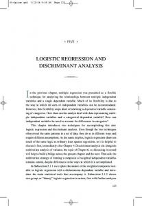
Figure 2. Left: cross correlation of up to 42 degrees. Each rows and columns are arranged in a vectorized fashion starting with (l, m) = (0, 0), (1, −1), (1, 0), (1, 1), · · · . Right: enlargement of small white square in the top left corner of the left figure. The average correlation is 0.16 and the most of correlations are extremely low indicating the independence of Fourier coefficients.

l=0 m=−l

which is spanned by up to k-th degree spherical harmonics. Let h0 be the solution of (1). Then the closest function h in the subspace Hk to h0 is given by k l  

e−l(l+1)σ plm Ylm (Ω) = arg min h − h0 . h∈Hk

l=0 m=−l

Unlike previous literature [1, 6, 8] that solves surface diffusion numerically using the finite difference scheme, Theorem 1 provides a new framework for performing surface diffusion by computing a series expansion. The advantage of this new framework is the ability to explicitly model surface diffusion using the Karhunen-Loeve expansion of a random field [22]. The Fourier coefficient vector plm can be modeled to follow independent multivariate normal N (μlm , D), where the covariance matrix is of the form 2 2 2 D = diag(σl1 , σl2 , σl3 ). Within the same degree, equal covariance is assumed. This model assumption is equivalent to the following. l k  

e−l(l+1)σ plm Ylm

l=0 m=−l

=

l k  

e−l(l+1)σ μlm Ylm

l=0 m=−l

+

l k  

e−l(l+1)σ lm Ylm ,

l=0 m=−l

where lm are independent multivariate normal ∼ N (0, D). The error term is the form of the Karhunen-Loeve expansion [22]. The normality assumption was tested using the Jarque-Bera statistic [20] for the parameters (k = 42, σ = 0.001) used in the study. For instance, 10 out of total (42 + 1)2 = 1, 849 Fourier coefficients of x-component in plm do not show normality at significance level α = 0.05.

Since uncorrelated Gaussian random variables are independent, we have also computed the cross correlation of all 18492 pairs of coefficients to check independence (Figure 2). Most pairs show very low correlation and the average correlation is 0.16 indicating the independence assumption is valid. The finite series expansion given in Theorem 1 is called the weighted spherical harmonic representation [7]. The weighted spherical harmonic representation shares similarity with the harmonic descriptors[14, 16, 28] which has been used to model simpler anatomical objects such as hippocampus [28] and ventricles [14] in brain imaging.

2.1. Model parameter estimation There are many available methods for computing Fourier coefficients [5, 14, 16, 28]; however, these methods are not suitable for computing the Fourier coefficients for a cortical mesh due to fairly large number of vertices. The fast Fourier transform [5, 16] usually needs a predefined regular grid so if the mesh topology is different for each cortical mesh, a time consuming interpolation is needed. The least squares method [14, 28] is also not suitable when the number of mesh vertices and the degree of the expansion are large. Consider the functional data f ∈ L2 (S 2 ). The functional data f is measured at the finite number of mesh vertices Ω1 , · · · , Ωn . Then the weighted Fourier series representation evaluated at Ωj is f (Ωj ) =

k l  

e−λ(λ+1)σ flm Ylm (Ωj ).

(5)

l=0 m=−l

The system of equations (5) can be written in a matrix form. Let f β

= (f (Ω1 ), · · · , f (Ωn )) = (f00 , f1,−1 , f1,0 , f1,1 , · · · , fkk ) .

Y

= (e−l(l+1)σ Ylm (Ωj )).

Matrix Y is the size of n × (k + 1)2 . The columns of Y are Y00 , Y1,−1 , Y1,0 , Y1,1 , · · · evaluated at Ω1 , · · · , Ωn . Then the system of equations (5) can be written as f = Yβ, where the Fourier coefficients are estimated as β = (Y Y)−1 Y f .

(6)

For most cortical surface segmentation algorithms [12, 23], n > 40, 000 and the matrix size can easily reach the physical memory limit of the most personal computers for k ≥ 42. To address this issue, we have developed an iterative method for solving a large least squares problem by decomposing it into smaller least squares problems [7]. The algorithm shares similarity to the matching pursuit method [24] in the underlying Hilbert space construction but differs in numerical implementation and motivation. While our algorithm was developed to avoid the computational burden of inverting a huge linear equation, the matching pursuit method was developed to compactly decompose a time frequency signal into a linear combination of pre-selected pool of basis functions. We briefly describe the algorithm. Initially, we estimate the first coefficient f00 by solving f (Ωj ) = f00 Y00 (Ωj ). If we let f 00 to be the least squares estimation, the next set of coefficients f1,−1 , f1,0 , f1,1 are estimated by solving f (Ωj ) − f 00 Y00 (Ωj ) =

1 

e−1(1+1)σ f1m Y1m (Ωj ).

m=−1

The subsequent set of coefficients f2,−2 , · · · , f2,2 are estimated by solving f (Ωj )−

l 1  

f lm Ylm (Ωj ) =

2 

2.2. Validation The weighed Fourier series representation is validated against analytically constructed ground truth. We have used the cortical thickness of a subject in constructing the analytical ground truth. Consider a surface measurement of the form l k   l=0 m=−l

Kσ ∗ g(Ω) =

βlm Ylm (Ω)

l k  

e−l(l+1)σ βlm Ylm (Ω).

(8)

l=0 m=−l

Using the sample cortical thickness data, we simulated the measurement of the form (7) by computing βlm = g, Ylm  (Figure 3 top left). Then we have compared the weighted Fourier series representation of g against the analytical ground truth (8) along the surface mesh (Figure 3). We have used σ = 0.001 and the corresponding optimal degree k = 42 [7]. The relative error is up to 0.013 at a certain vertex and the mean relative error over all mesh vertices is 0.0012. Our validation results demonstrates that the numerical implementation of the weighted Fourier series representation is sufficiently good.

Surface Asymmetry Analysis

3.1. Correspondence across hemispheres

At each iteration, the residual of the previous fit is used to estimate the next set of coefficients. The process continues until the residual is no longer statistically significant. At the l-th iteration, the iterative algorithm inverts manageable smaller (2l − 1)× (2l − 1) matrix instead of huge (k + 1)2 × (k + 1)2 matrix in (6).

g(Ω) =

for given βlm . Heat kernel smoothing of g is given as an exact analytic form, which serves as the ground truth for validation:

e−2(2+1)σ f2m Y2m (Ωj ). 3. Local

m=−2

l=0 m=−l

Figure 3. Cortical thickness is simulated from the sample cortical thickness. The ground truth is analytically constructed from the simulation. Then the weighted Fourier series representation are compared against the ground truth. The mean relative error is at 0.0012.

(7)

Comparing measurements defined at different cortical surfaces is not a trivial task due to the fact that no two cortical surfaces are identically shaped. We need to establish surface correspondence between hemispheres and between subjects for subsequent statistical analysis. We present a new surface registration technique utilizing the Hilbert space property of spherical harmonics. Consider pa and q  obtained from coordinates p and q rameterizations p respectively:  (Ω) = p

l k  

e−l(l+1)σ plm Ylm (Ω),

l=0 m=−l

(Ω) = q

l k   l=0 m=−l

e−l(l+1)σ qlm Ylm (Ω).

Figure 4. Representative subjects showing cortical thickness (g), its weighted-SPHARM representation (b g ), asymmetry index (A), symmetry index (S) and normalized asymmetry index (N ). The Cortical thickness is projected onto the original brain surfaces while all other measurements are projected onto the 42-th degree weighed Fourier series representation.

 is deformed to p  + d, where d = Suppose the surface p (dj ) is the displacement vector field to be estimated. We find optimal displacement d that minimizes the discrepancy  +d and q  in the finite subspace Hk using the L2 between p norm:

Proof. From the way the spherical coordinates are set up (Figure 1), we obtain  ∗ (θ, ϕ) p

 (θ, 2π − ϕ) = p =

k l  

e−l(l+1)σ plm Ylm (θ, 2π − ϕ)

l=0 m=−l

 and q , the optimal Theorem 2 Given parameterization p  is  to q displacement from p k 

l 

e

−l(l+1)σ

l=0 m=−l

(qlm −plm )Ylm = arg min  p+d− q. dj ∈Hk

Theorem 2 shows that the optimal displacement is obtained by taking the difference between two parametric representations and matching coefficients of the same degree and order. Note that we are not taking the difference between the original noisy surface meshes. Theorem 2 can be further used to establish the inter-hemispheric correspon.  to be the mirror reflection of p dence by letting q

 ∗ denotes the mirror reflection of p  with reTheorem 3 If p spect to the midsaggital cross section, the optimal displace ∗ is  to p ment from p

−2

l k   l=0 m=0

 ∗ . e−l(l+1)σ plm Ylm = arg min  p+d−p dj ∈Hk

=

k −1  

e−l(l+1)σ plm Ylm (θ, ϕ)

l=0 m=−l

−

l k  

e−l(l+1)σ plm Ylm (θ, ϕ).

l=0 m=0

The last decomposition into negative and positive orders is obtained from the property of spherical harmonics:  −Ylm (θ, ϕ), −l ≤ m ≤ −1, Ylm (θ, 2π − ϕ) = (9) Ylm (θ, ϕ), 0 ≤ m ≤ l. =p  ∗ , we obtain the result.  Then letting q Theorem 3 shows that the optimal inter-hemispheric correspondence is obtained by matching the parameterization  (θ, 2π − ϕ). Again note that we are not try (θ, ϕ) to p p ing to match the original mesh coordinates p(θ, ϕ) but their algebraic representations.

3.2. Local asymmetry index Theorem 3 enables us to establish the inter-hemispheric correspondence and, in turn, to construct cortical thickness based asymmetry index. Now we present our main contribution.

Theorem 4 If g is the weighted spherical harmonic representation of cortical thickness, the normalized asymmetry index of type (L-R)/(L+R) is given by k N (θ, ϕ) =

−1

l=1 k l=0

m=−l

l

m=0

e−1(l+1)σ glm Ylm (θ, ϕ) e−l(l+1)σ glm Ylm (θ, ϕ)

. (10)

 (θ, ϕ), we have cortical thickProof. At each position p ness g(θ, ϕ). Then from Theorem 3, we match  g(θ, ϕ) to g(θ, 2π − ϕ) for the hemispheric correspondence. From  (9), we obtain −1 k  

g(θ, 2π − ϕ) =

e−1(l+1)σ glm Ylm (θ, ϕ)

Figure 5. Discriminant power projected on top of the average cortical surface. The discriminant power ranges from 32.1 to 85.7%. The logistic discriminant analysis framework provides an alternative to the traditional corrected P-value approach in the two group comparison setting.

l=1 m=−l l k  

−

e−l(l+1)σ glm Ylm (θ, ϕ)

l=0 m=0

Comparing the expansions g(θ, ϕ) and g(θ, 2π − ϕ), we see that the negative order terms are invariant while the positive order terms change the sign. Computing N (θ, ϕ) =

g(θ, ϕ) −  g(θ, 2π − ϕ) g(θ, ϕ) +  g(θ, 2π − ϕ)

directly, we obtain the result.  The numerator in the expression (10) is the sum of all negative orders while the denominator is the sum of all positive and the 0-th orders. The larger the value of the index, the larger the amount of asymmetry. Following the proof of Theorem 4,  g(θ, ϕ) can be decomposed into symmetric S and antisymmetric A parts so that g(θ, ϕ) = S(θ, ϕ) + A(θ, ϕ), where S(θ, ϕ)

= =

1 g(θ, ϕ) + g(θ, 2π − ϕ) 2 −1 k   e−1(l+1)σ glm Ylm (θ, ϕ) l=1 m=−l

and A(θ, ϕ)

1 g(θ, ϕ) − g(θ, 2π − ϕ) 2 l k   e−l(l+1)σ glm Ylm (θ, ϕ). = =

l=0 m=0

Figure 4 shows the asymmetry index for selective subjects.

3.3. Local discriminant analysis For each subject, its normalized asymmetry index N (θ, ϕ) is computed and modeled as a zero mean Gaussian

random field. For the traditional group comparison between autistic and normal control subjects, the T statistic at each point (θ, ϕ) would be constructed. Since T statistics at different points are correlated, it becomes a multiple comparison problem [4, 26, 31]. The corrected P-value accounting for spatially correlated test statistics is determined by computing the superima distribution of the T random field [31], i.e.

(11) P sup T (θ, ϕ) < h . (θ,ϕ)∈S 2

Unfortunately, computing the suprima distribution of the T random field is not an easy task and requires satisfying many distributional assumptions and the estimation of the smoothness of the random field. If we can come up with a different framework that does not use the traditional hypothesis testing paradigm, there is no need to compute the P-value. With this as a motivation, we propose a different approach called the logistic discriminant analysis [13, 18] that does not require computing the P-value and still is able to detect the regions of abnormal asymmetry pattern in the autistic subjects. Unlike previous discriminant techniques [19, 28, 29] that tried to classify preselected feature vectors, our approach does not require any preselected feature vectors and performs the classification at each mesh vertex. Let ni (θ, ϕ) denotes the normalized asymmetry index for the i-th subject at a particular point (θ, ϕ). Let Yi (θ, ϕ) be the clinical state of the i-th subject modeled as a Bernoulli random variable with parameter πi (θ, ϕ). Yi = 1 if the i-th subject is autistic with probability πi while Yi = 0 if the subject is normal with probability 1 − πi . Then we have the following logistic model at each point (θ, ϕ), which links the probability of clinical statue πi to the asymmetry index ni : log

πi = β0 + β 1 n i . 1 − πi

(12)

The unknown parameters β(θ, ϕ) = (β0 , β1 ) are estimated by maximizing the loglikelihood function L(β) at

each point (θ, ϕ). The loglikelihood function is given by log L(β) = const. +

n 

yi (β0 + β1 ni ) + log(1 − πi ). (13)

i=1

Since the loglikelihood function (13) is not easy to maximize analytically, the Newton-Raphson method is used to maximize it in an iterative fashion. Starting with an arbitrary initial vector β 0 , we estimate iteratively β j+1 = β j + I(β j )−1

∂ log L(β) j (β ), ∂β

where I is the Fisher information matrix [13, 18]. Once we estimated the parameters β(θ, ϕ), we classify the i-th subject as autistic if P (Yi = 1) > P (Yi = 0), which is equivalent to the condition πi > 1/2. The classification error rate γ(θ, ϕ) is estimated by the leave-one-out cross-validation scheme. Denote e−i (θ, ϕ) as the error rate for leaving the i-th subject out. Note that e−i = 0 if the subject is classified correctly while e−i = 1 if the subject is misclassified. Then the error rate γ is estimated as 1 e−i . n i=1 n

γ (θ, ϕ) =

The discriminant power is then given as 1 − γ  and it is displayed in Figure 5 localizing the regions of abnormal asymmetry pattern in autistic subjects. In order to show that the discriminant power map can be used as an alterative to the usual P-value map, the statistical significance of discriminant power is computed using Presss Q-statistic n(2ˆ γ − 1)2 , which is asymptotically 2 distributed as χ1 [17]. Figure 6 shows the plot of P-value of Presss Q-statistic as a function of discriminant power. Larger discriminant power corresponds to smaller P-value. For n = 28, the discriminant power of 0.85 corresponds to the extremely small P-value of 0.0002. To account for multiple comparisons, this small P-value needed to be corrected by computing the probability of the superima distribution of a test statistic similar to (11). However, this is not so trivial. On the other hand, the proposed discriminant power approach is much easier.

4. Application Three Tesla T1 -weighted MR scans were acquired for 16 high functioning autistic and 12 control right handed males. The autistic subjects were diagnosed by a trained and certified psychologist [10]. The average ages are 17.1 ± 2.8 and 16.1 ± 4.5 for control and autistic groups respectively. The standard image processing steps, such as the intensity non-uniformity correction and the global affine normalization into the Montreal neurological institute stereotaxic

Figure 6. The plot of statistical significance as a function of discriminant power for various sample size n = 10, 28, 100.

space, were performed. Afterwards, an automatic tissuesegmentation algorithm based on a supervised artificial neural network classifier was used to segment gray and white matters. Cortical surface meshes were constructed by a deformable surface algorithm and cortical thickness g and mesh vertices p are obtained. Using the bijective mapping from the unit sphere to the cortical surface, mesh vertices p were parameterized by Euler angles (θ, ϕ) (Figure 1).  and The weighted spherical harmonic representation p g for 28 subjects was constructed using the iterative algo rithm with bandwidth σ = 0.001 corresponding to k = 42 degrees (Figure 4). The representation has been validated against the ground truth and shown to perform sufficiently well with the average relative error of 0.0012 (Figure 3). The symmetry (S), asymmetry (A) and normalized asymmetry (N ) indices were computed and projected onto k = 42 degree representation (Figure 4). The normalized asymmetry index was used in localizing the regions of cortical asymmetry difference between two groups. Instead of performing the usual two sample T-test, which introduces multiple comparison issues [4, 26, 31], logistic discriminant analysis was performed. At each point, the logistic model (12) was fitted to link the probability of clinical status to the asymmetry index. The logistic model was used to estimate the probability of the asymmetry index belonging to the autistic group. Then we computed the discriminant power, which is defined as the rate of correct classification. The discriminant power was projected onto the average cortical surface constructed by averaging the Fourier coefficients of all subjects within the same spherical harmonics basis using Theorem 2 (Figure 5). The average surface serves as an anatomical landmark for displaying these indices as well as projecting the logistic discriminant analysis result. The regions of high discriminant power indicates the likelihood of the regions to exhibit abnormal asymmetry

in the autistic subjects.

References [1] A. Andrade, F. Kherif, J. Mangin, K. Worsley, A. Paradis, O. Simon, S. Dehaene, D. Le Bihan, and J.-B. Poline. Detection of fmri activation using cortical surface mapping. Human Brain Mapping, 12:79–93, 2001. [2] T. Barrick, C. Mackay, S. Prima, F. maes, D. Vandermeulen, T. Crow, and N. Roberts. Automatic analysis of cerebral asymmetry: an exploratory study of the relationship between brain torgue and planum temporale asymmetry. NeuroImage, 24:678–691, 2005. [3] P. Barta, M. Miller, and A. Qiu. A stochastic model for studying the laminar structure of cortex from mri. IEEE Transactions on Medical Imaging, 24:728–742, 2005. [4] Y. Benjamini and Y. Hochberg. Controlling the false discovery rate: a practical and powerful approach to multiple testing. J. R. Stat. Soc, Ser. B, 57:289–300, 1995. [5] T. Bulow. Spherical diffusion for 3d surface smoothing. IEEE Transactions on Pattern Analysis and Machine Intelligence, 26:1650–1654, 2004. [6] A. Cachia, J.-F. Mangin, D. Riviere, F. Kherif, N. Boddaert, A. Andrade, D. Papadopoulos-Orfanos, J.-B. Poline, I. Bloch, M. Zilbovicius, P. Sonigo, F. Brunelle, and J. . Regis. A primal sketch of the cortex mean curvature: a morphogenesis based approach to study the variability of the folding patterns. IEEE Transactions on Medical Imaging, 22:754–765, 2003. [7] M. Chung, K. Dalton, L. Shen, A. Evans, and R. Davidson. Weighted fourier representation and its application to quantifying the amount of gray matter. IEEE Transactions on Medical Imaging, 26:566–581, 2007. [8] M. Chung, K. Worsley, T. Paus, D. Cherif, C. Collins, J. Giedd, J. Rapoport, , and A. Evans. A unified statistical approach to deformation-based morphometry. NeuroImage, 14:595–606, 2001. [9] R. Courant and D. Hilbert. Methods of Mathematical Physics: Volume II. Interscience, New York, english edition, 1953. [10] K. Dalton, B. Nacewicz, T. Johnstone, H. Schaefer, M. Gernsbacher, H. Goldsmith, A. Alexander, and R. Davidson. Gaze fixation and the neural circuitry of face processing in autism. Nature Neuroscience, 8:519–526, 2005. [11] C. Davatzikos. Spatial transformation and registration of brain images using elastically deformable models. Comput. Vis. Image Underst., 66:207–222, 1997. [12] B. Fischl, M. Sereno, R. Tootell, and A. Dale. Highresolution intersubject averaging and a coordinate system for the cortical surface. Hum. Brain Mapping, 8:272–284, 1999. [13] B. Flury. A First Course in Multivariate Statistics. Springer, 1997. [14] G. Gerig, M. Styner, D. Jones, D. Weinberger, and J. Lieberman. Shape analysis of brain ventricles using spharm. In MMBIA, pages 171–178, 2001. [15] G. Gerig, M. Styner, M. Shenton, and J. Lieberman. Shape versus size: improved understanding of the morphology of brain structures. In MICCAI, pages 24–32, 2001.

[16] X. Gu, Y. Wang, T. Chan, T. Thompson, and S. Yau. Genus zero surface conformal mapping and its application to brain surface mapping. IEEE Transactions on Medical Imaging, 23:1–10, 2004. [17] J. Hair, R. Anderson, R. Tatham, and W. Black. Multivariate data analysis. Prentice Hall, Inc., 1998. [18] T. Hastie, R. Tibshirani, and J. Friedman. The elements of statistical learning. Springer, 2003. [19] R. Higdon, N. Foster, R. Koeppe, C. DeCarli, W. Jagust, C. Clark, N. Barbas, S. Arnold, J. H. R.S. Turner, and S. Minoshima. A comparison of classification methods for differentiating fronto-temporal dementia from alzheimer’s disease using fdg-pet imaging. Stat Med, 23:315–326, 2004. [20] C. Jarque and A. Bera. A test for normality of observations and regression residuals. International Statistical Review, 55:1–10, 1987. [21] D. Kennedy, K. O’Craven, B. Ticho, A. Goldstein, N. Makris, and J. Henson. Structural and functional brain asymmetries in human situs inversus totalis. Neurology, 53:1260–1265, 1999. [22] J. Li and A. Hero. A spectral approach to statistical polar shape modeling. In Proceedings of International Conference on Image Processing, 2002. [23] J. MacDonald, N. Kabani, D. Avis, and A. Evans. Automated 3-D extraction of inner and outer surfaces of cerebral cortex from mri. NeuroImage, 12:340–356, 2000. [24] S. Mallat and Z. Zhang. Matching pursuits with timefrequency dictionaries. IEEE Transactions on Signal Processing, 41:3397–3415, 1993. [25] M. Miller, A. Banerjee, G. Christensen, S. Joshi, N. Khaneja, U. Grenander, and L. Matejic. Statistical methods in computational anatomy. Statistical Methods in Medical Research, 6:267–299, 1997. [26] T. Nichols and S. Hayasaka. Controlling the familywise error rate in functional neuroimaging: a comparative review. Stat Methods Med. Res., 12:419–446, 2003. [27] S. Rosenberg. The Laplacian on a Riemannian Manifold. Cambridge University Press, 1997. [28] L. Shen, J. Ford, F. Makedon, and A. Saykin. surface-based approach for classification of 3d neuroanatomical structures. Intelligent Data Analysis, 8:519–542, 2004. [29] C. Thomaz, J. Boardman, S. Counsell, D. Hill, J. Hajnal, A. Edwards, M. Rutherford, D. Gillies, and D. Rueckert. A whole brain morphometric analysis of changes associated with preterm birth. In SPIE Medical Imaging 2006: Image Processing, volume 6144, pages 1903–1910, 2006. [30] P. Thompson and A. Toga. A surface-based technique for warping 3-dimensional images of the brain. IEEE Transactions on Medical Imaging, 15, 1996. [31] K. Worsley, S. Marrett, P. Neelin, A. Vandal, K. Friston, and A. Evans. A unified statistical approach for determining significant signals in images of cerebral activation. Human Brain Mapping, 4:58–73, 1996.