This article has been accepted for publication in a future issue of this journal, but has not been fully edited. Content may change prior to final publication. Citation information: DOI 10.1109/TBME.2014.2366554, IEEE Transactions on Biomedical Engineering IEEE TRANSACTIONS ON BIOMEDICAL ENGINEERING, VOL. XX, NO. X, JAN 201X
1
Quantifying Electrode Reliability During Brain-Computer Interface Operation Hesam Sagha, Serafeim Perdikis, Jos´e del R. Mill´an, and Ricardo Chavarriaga
Abstract—One of the problems of non-invasive BrainComputer Interface (BCI) applications is the occurrence of anomalous (unexpected) signals that might degrade BCI performance. This situation might slip the operator’s attention since raw signals are not usually continuously visualized and monitored during BCI-actuated device operation. Anomalous data can for instance be the result of electrode misplacement, degrading impedance or loss of connectivity. Since this problem can develop at run-time, there is a need of a systematic approach to evaluate electrode reliability during online BCI operation. In this paper, we propose two metrics detecting how much each channel is deviating from its expected behavior. This quantifies electrode reliability at run-time which could be embedded into BCI data processing to increase performance. We assess the effectiveness of these metrics in quantifying signal degradation by conducting three experiments: electrode swap, electrode manipulation and offline artificially degradation of P300 signals. Keywords-Brain Computer Interaction, Anomaly Detection, Electrode Reliability
I. I NTRODUCTION Brain-Computer Interfaces (BCIs) provide the possibility of a direct, non-muscular communication and control channel by recognizing patterns of brain activity [1]. The most common recording technique used for these devices is the electroencephalography (EEG). This is due to its high temporal resolution, portability and relative low cost [2]. However, this technique is characterized by low spatial resolution, since the neural activity is propagated through the brain tissue and scalp which acts as a low-pass filter and smears the activity [3]. Moreover, it is prone to contamination due to muscular artifacts and electromagnetic noise, resulting in a low signalto-noise ratio. Furthermore, modifications in the recording settings, e.g., changes in conductivity [4], result in signal variations that may also affect the decoding performance. Despite these drawbacks, complex BCI applications have been designed including virtual keyboards [5], quadcopter [6], wheelchairs [7] and neuroprostheses [8]. Some of these systems –relying on both neural evoked responses (e.g., P300based BCI) or modulation of sensory-motor rhythms (e.g., Motor imagery (MI)-based BCI)– have successfully been tested Manuscript received November 19,2013; revised February 15, 2014, May 5,2014 and September 29, 2014; accepted October 25, 2014. Date of publication XX X, 2014; date of current version XX X, 2014. This work was supported by the European projects OPPORTUNITY (FET 225938) and TOBI (ICT FP7-224631) All authors are with Chair in Non-Invasive Brain-Machine Interface, Center ´ for Neuroprosthetics Ecole Polytechnique F´ed´erale de Lausanne, EPFL-STICNBI, Station 11, CH-1015, Lausanne, Switzerland. e-mail: Hesam Sagha:
[email protected], other authors: {name.surname}@epfl.ch Copyright (c) 2013 IEEE. Personal use of this material is permitted. However, permission to use this material for any other purposes must be obtained from the IEEE by sending an email to
[email protected]
by end-users in research labs, clinics and at their homes. However, several aspects undermine the possibility of having a wider deployment, as well as sustainable, successful, longterm use by end-users (i.e. patients, caretakers, etc.) [4]. This includes the variability in the system performance, difficulties in system setup and calibration, that often requires intervention of qualified personnel. One of the causes for performance variability is the non-stationarity of brain signals in general and EEG in particular [1], [9]. For this reason the models obtained from the calibration data do not necessarily suit the signals obtained during operation. This can be due to changes in the brain activity patterns (e.g., resulting from brain plasticity [10], development of new strategies by the user during feedback sessions [11]). Several pre-processing and classification techniques can be applied to make the system less-sensitive to these factors (e.g., averaging over trials [12], evidence accumulation [4]). In addition, adaptive methods have been proposed to alleviate this problem [9], [13]. Another source of variability concerns the characteristics, setting up and the placement of the sensors [4], [14]. Since it is impossible to replicate and maintain exactly the same recording conditions (e.g., electrode position, impedance, physiological or electrical artifacts), these variations cannot be avoided and may appear both across and within recording sessions. For this reason, classifier adaptation may not be ideal, as it may attempt to track irregular task-unrelated data streams. As an alternative, methods that assess the electrode reliability can be applied to identify these anomalies, allowing to take appropriate measures to compensate for their effects. In this paper we propose two metrics based on the local correlation and mutual information between electrodes, respectively. Experimental results show that they successfully detect anomalous EEG patterns irrespective of their anomaly cause (e.g., montage errors, impedance change, artifacts). Although we report results using scalp EEG recordings, the proposed approaches can be used for other recording techniques, e.g., Electrocorticography (ECoG). The rest of this paper is organized as follows; first we present related work on anomaly detection, followed by the description of the proposed method. Then we describe the performed experiments (Section IV) and report the obtained results (Section V). Finally, we present our conclusions and the proposed future work in this direction. II. R ELATED WORKS Detection of anomalous data patterns has been largely addressed in fields like control systems [15] and remote sensing [16]. However, this issue has been largely neglected in the
0018-9294 (c) 2013 IEEE. Personal use is permitted, but republication/redistribution requires IEEE permission. See http://www.ieee.org/publications_standards/publications/rights/index.html for more information.
This article has been accepted for publication in a future issue of this journal, but has not been fully edited. Content may change prior to final publication. Citation information: DOI 10.1109/TBME.2014.2366554, IEEE Transactions on Biomedical Engineering IEEE TRANSACTIONS ON BIOMEDICAL ENGINEERING, VOL. XX, NO. X, JAN 201X
2
III. M ETHOD
Fig. 1. Left) Example of data distribution (black) and an anomalous data point (star shape) with a single anomalous feature (z). Right) Histogram of marginal distributions of the data on each axis.
design of BCI applications. In this field, most efforts have been devoted to specifically cope with recording contamination by muscular activity or eye movements [17]. The most common techniques are based on independent component analysis (ICA) or linear filtering of patterns previously identified as signatures of the artifact [18]. Albeit effective, these approaches are specifically tailored for such artifacts and are not suitable for other anomalies. Methods for anomaly detection are surveyed in [19]. These methods typically indicate whether the data pattern is anomalous, without identifying which of its components (i.e. features) is responsible for the anomaly. As an illustration, Fig. 1(left) shows a hypothetical multivariate normal data distribution with three features, centered at µ = [x : 0, y : 0 , z : 0]. An anomalous sample at X 0 = [0, 0, 1.3] (shown as a square dot) deviates from the distribution solely due the value of feature z. The methods reviewed in [19] will label the pattern vector as anomalous without being able to specifically identify that feature Xz0 is responsible for the anomaly. Such methods are not suitable for BCI since they would consider the whole sample as anomalous, despite the fact that two of its features still provide valuable information. A simple approach would be to keep track of data statistics individually on each channel [20] and consider deviations from those feature-specific estimates as anomalies [21]. However, since in this case deviations are monitored on each channel separately, there is an implicit assumption of feature independence that may not hold. Revisiting the previous example, Fig. 1(right) depicts the histogram of marginal distributions of the same dataset. Looking at the anomalous feature alone (Xz0 = 1.3) would not substantiate that the detected deviation corresponds to an anomaly. However the exemplary data distribution shows high correlations among features; i.e. such a feature value would only be valid if other features fall in a particular part of the feature space (e.g., [x : 1.3, y : 1.3, z : 1.3]). Indeed this is the case for EEG where signals of nearby electrodes tend to be highly correlated. Furthermore, in the case of EEG-based BCI certain anomalies do not change the statistics of the individual signals (e.g., electrodes are misplaced). Therefore, they cannot be detected by this type of methods. An alternative approach, presented in the next section, is to evaluate the behavior of each electrode with respect to the other electrodes. That is, take into account correlations across electrodes to reach better detection of anomalous patterns.
As mentioned above, the proposed method relies on the relation of a given electrode to other channels in the system. At run time, larger changes of this relation –compared to calibration data– can be considered as a marker of decreased electrode reliability. Since the method is based on the relation across channels, it is well suited for EEG or ECoG signals where volume conduction induces high correlations. However, since it is based on changes on this relation, it also can be applied in less correlated signals. To assess these changes we present two different metrics: The first one based on the Mahalanobis distance (section III-A), while the second is based on the mutual information between channels (section III-B). To compare the proposed approaches we also assessed three other metrics as reference. These are techniques based on Laplacian spatial filtering (section III-C), the signal statistics (section III-D) and offset value (section III-E). A. Distance-based approach (DB) We want to assess whether a given channel exhibits the same behavior as observed in the training phase. To this end, we exploit the fact that EEG signals are not independent and correlations can be found among channels (especially neighboring electrodes). The rationale of this approach is to estimate the expected value at a given channel using the measures from its neighbors and their cross-correlation. We can then monitor the distance between the predicted value and the actual measure. Assuming the data are normally distributed, for a given channel, e, the expected value, vˆe , can be obtained using the conditional mean based on the measures from neighboring channels values, vne : vˆe = µe||vne = µe + Σene Σ−1 ne ne (vne − µne )
(1)
where µe is the mean value of the channel of interest, while µne is the mean vector corresponding to neighboring channels. Σene is the covariance between the electrode e and its neighbors, and finally Σne ne is the covariance among the neighboring electrodes. All these values are computed on the training dataset. The distance between the expected value vˆe and the current measure, ve , is estimated using the Mahalanobis distance since it takes the shape of the distribution of the difference into account: 2 2 DeviationM (2) e = (ve − vˆe ) /σe where σe2 is the variance of the distance for channel e. As mentioned above, the expected signal vˆe depends on the measures on other channels. However, these channels can also be faulty (unreliable), thus affecting the process and decreasing the quantification accuracy. In order to prune unreliable channels from the estimation, we first rank the channels as follows. Starting from a vector, vene , composed of the values of the current channel and its neighbors, we iteratively remove the channel, c, in the set which leads to the least Mahalanobis distance to the mean value, µene , in the k-1 dimensional space: −1
c Dc = (ven − µcene )T (Σcene ) e
c (ven − µcene ) e
0018-9294 (c) 2013 IEEE. Personal use is permitted, but republication/redistribution requires IEEE permission. See http://www.ieee.org/publications_standards/publications/rights/index.html for more information.
(3)
This article has been accepted for publication in a future issue of this journal, but has not been fully edited. Content may change prior to final publication. Citation information: DOI 10.1109/TBME.2014.2366554, IEEE Transactions on Biomedical Engineering IEEE TRANSACTIONS ON BIOMEDICAL ENGINEERING, VOL. XX, NO. X, JAN 201X
Algorithm 1 Detection of anomalous electrodes. Estimate Σ, µ, σe2 and statistics on D using training set for Each electrode, e do eList ← Select the electrode, e and its neighbors, ne , in the radius of Rpr. RANKING PHASE: CorrectList ← eList for i=1:length(ne ) do for each c ∈ CorrectList do others ← CorrectList − c Dc = MahalDistance(vothers ,Σothers ,µothers ) end for anomal = argminc (Dc ) CorrectList ← CorrectList − anomal rank(i) = anomal end for REGENERATION PHASE ind = f indind(rank, e) hE = rank(j) such that j > ind vˆe = regenerate(vhE , µe∪hE , Σe∪hE ) (1) Dif fe = ve − vˆe M T rain Deviatione = Dif fe /var(Dif fe ) (2) end for
(3)
where the superscript c indicates removing the element c from a vector or removing the corresponding row and column from the covariance matrix. In this case, the value of the distance metric in the k − 1 dimension indicates how much the value of the corresponding data element, c, is outside the estimated distribution. Lower value in k − 1 dimension means the element c is farther from its expected value. Channels are thus ranked according to the order in which they were removed, with the lowest ranking corresponding to the first removed channels. For example, in the case shown in Fig 1, removal of the z dimension reduces the Mahalanobis distance of the point [x : 0, y : 0] to zero, while removing other axes yields larger distances. After the ranking procedure, only those channels that are better ranked than the channel of interest are used to compute the expected value, vˆe (1). Then, we estimate the distance to the actual measure using (2). Since electrodes are highly correlated with its surrounding neighbors, the estimation process considers only the nearest electrodes. The size of the neighborhood is defined by the radius Rpr, as illustrated in Fig. 2(b). The final algorithm is shown in Algorithm Box 1. The function f indind(rank, e) returns the index of the electrode e in the rank list. hE includes the electrodes which seem to be less faulty. In order to obtain a more robust estimation we compute the M \ e , of the distance DeviationM moving average, Deviation e over a sliding window of size win. Nevertheless, the length of the window induces proportional time lags on the detection. 1) Computational cost: For a given channel, there are two phases. First, the ranking phase estimates the Mahalanobis distance in k-1 dimensions. Each distance calculation involves three matrix multiplications which cost O(Nn3e ). Therefore, the complexity of the first phase is O(Nn4e ). The next phase requires three matrix multiplications and two matrix summations for the electrodes in the higher ranks (at most ne ), therefore it yields a complexity of O(Nn4e ), the same holds for the distance estimation. So, the final order of complexity is O(N Nn4e ), where N is the total number of electrodes.
3
B. Information theoretic approach (IT) In this case, we characterize the deviation of the signal based on the pairwise mutual information between channels. To extract mutual information, the signals are quantized into predefined bins. These bins are defined automatically based on Sturges’ criterion. The mutual information between channels n and m is computed as: X X p(x, y) (4) p(x, y)log Inm = p(x)p(y) x∈binn y∈binm
We estimate then the difference between the mutual informatest tion, Inm , computed in the current samples over a window of length win and that computed on the training data. test train Dif fnm = Inm − Inm
(5)
To remove the effect of common changes affecting all electrodes, the deviation is computed as the distance to the average value of the all differences, Dif f , and summed over all the electrodes. X (6) DeviationIn = (Dif fnm − Dif f )2 m6=n
This approach does not need a smoothing procedure since mutual information is already computed over a window of samples. 1) Computational cost: Computing I for two electrodes has a complexity of order O(b2 win), where b is the number of bins, and win is the size of the sliding window. Therefore, the computation of I for all the electrodes costs O(b2 N 2 win). Computing Dif f and Deviation is not demanding and has the order of O(N 2 ). This is lower than the cost of the method based on the Mahalanobis distance. C. Laplacian approach In this case, the deviation is equivalent to a Laplacian spatial filter, i.e. the average of values of the neighborhood electrodes is subtracted to the captured value: 1 X DeviationL vne )2 (7) n = (vn − ne n e
As before, we use a window to smooth the deviation values. D. Statistic-based approach In this case, anomalies are detected based on the statistics of the signal [20]. They comprise maximum value, standard deviation, kurtosis and skewness of the signal in Alpha band [8-12] Hz, Beta band [13-35] Hz and high-passed signal (> 1 Hz). In addition, given their use as features for BCI applications, we also considered power spectral densities computed in the range of [1-40] Hz [4]. This yields 52 values for each window of data (win = 2s, overlap = 1s). To detect anomalies, the statistics which exceed the 5%-quantile of the statistics obtained in the training set are spotted as anomaly. Finally we add up all the decisions for all statistics, leading an integer value between 0 and 52. DeviationSn =
52 X
outlierin
i=1
0018-9294 (c) 2013 IEEE. Personal use is permitted, but republication/redistribution requires IEEE permission. See http://www.ieee.org/publications_standards/publications/rights/index.html for more information.
(8)
This article has been accepted for publication in a future issue of this journal, but has not been fully edited. Content may change prior to final publication. Citation information: DOI 10.1109/TBME.2014.2366554, IEEE Transactions on Biomedical Engineering IEEE TRANSACTIONS ON BIOMEDICAL ENGINEERING, VOL. XX, NO. X, JAN 201X
4
where outlieri is 1 when the ith statistics for nth electrode exceeds the 5%-quantile. As before, we also use a window to smooth decisions. E. Signal offset We finally estimate another metric based on variations of the offset (DC) value of the signal. This measure is related to the conductivity of an electrode. To detect changes during the online runs, we compare this DC value between two consecutive time windows. IV. E XPERIMENTS We report results on three different experiments using real EEG recordings. The first one emulates electrode misplacement, i.e. swapping the location of two neighboring electrodes, which is a possible mistake in the recording setup, especially when the system is deployed out of research laboratories [4]. This experiment was performed on pre-recorded data for a Motor-imagery (MI) based BCI. In the second scenario, we deliberately manipulated the electrodes during a recording of 64 EEG channels to induce anomalies in a controlled manner. The third experiment aims at assessing the effect of noise on P300 classifier performance and the detection such anomalies. The proposed methods are independent of the choice of preprocessing and feature extraction methods. Except for the statistics- and offset-based approaches, we filtered the signal of both experiments in the band 4 − 24Hz, since the neural substrates of most BCI tasks are cortical rhythms within this range. This reduces the noise and allows better estimation of covariance matrices and distances. Furthermore, it should be noted that the anomaly detection does not have to be applied at the same sampling frequency as the EEG acquisition or the BCI application. We thus downsampled the data and took into account samples acquired every 175 ms. Unless stated otherwise, the smoothing window, win, used to compute the deviation comprised 200 samples, equivalent to 35s of data. A. Experiment I - Swapping electrodes Quantifying reliability of swapped electrodes from the signal characteristics is a difficult task. In particular, due to the fact that the recorded signals still correspond to normal EEG patterns. Furthermore, in the case of nearby electrodes, signals in both channels will be highly correlated. In consequence, quantification based on single channel statistics usually fail to identify this type of anomalies. In this experiment we emulate the swap of electrode position while the subject is performing a 2-class Motor Imagery task, Fig. 2(a) (cf. [4]). Analysis was done offline from prerecorded data. EEG is recorded on 16-electrodes at a sampling frequency of 256Hz using a g.USBamps system (gTec medical engineering, Schiedelberg, Austria) as shown in Fig. 2(b). We analyzed the data of 12 able-bodied subjects performing two BCI sessions over different days. One session is used for training and the other one for testing. For each subject we estimate the deviation values after swapping a pair of electrodes selected at random among nearby electrodes (radius
(a)
(b)
Fig. 2. (a) Motor imagery experimental protocol. Arrow bars in the bottom show the feedback provided to the user. Adapted from [4]. (b) EEG montage used in the Motor-imagery experiment. Electrodes in the square are within the radius Rpr = 1. Shaded electrodes correspond to radius Rpr = 2 for electrode C2.
Rsw = 1), as well as for more distant ones (Rsw = 2). This procedure was repeated 5 times for each case, and results are reported for processing radius (Rpr) equal to 1 and 2. B. Experiment II - Controlled scenario In this experiment we devised a scenario comprising possible anomalies during EEG recording, e.g., electrode failure, impedance change, disconnection and misplacement. In the experiment we recorded spontaneous EEG of five able-bodied subjects during resting condition. The recording was done with a 64-electrode Biosemi ActiveTwo system (Biosemi, Amsterdam, the Netherlands), in an extended 10/20 montage, at a sampling frequency of 2048Hz. We used the same preprocessing and window length as for the previous experiment and Rpr = 1. The first 5 minutes of the recording were used as training set. Then, we artificially introduce anomalies by physical manipulation of the electrodes. This phase, lasting another 5 minutes, was used as testing set. The scenario is as follows: a) No anomaly (30s) b) Electrode C4 was pressed by the operator c) Electrode Cz was pressed (30s) d) Disconnect FC2, electrode is left floating (60s) e) Disconnect FCz. FC2 is left floating (60s) f) Swap FC2 and FCz (60s) g) Electrode F5 was pressed (30s) By pressing an electrode we are emulating changes in the conductivity and possible external artifacts. C. Experiment III - P300 classification Arguably, most of the BCI systems used currently by patients with disabilities are based on the decoding of the P300-signal. Here, we analyze how the noise level affects the performance of such systems, and the possibility of quantifying this level using one of the proposed techniques (IT-based measure). We analyzed data from a P300 domotic application [12]. Eight subjects took part in the experiment, four are healthy and four are disabled wheelchair-bounded with some limited abilities in their hand movements. The experiment comprises a total of four sessions across two days, yielding on average 3420 trials per subject. Common Average Referencing (CAR) is used followed by bandpass filtering 112Hz and then data is downsampled to 64Hz. Each one-second
0018-9294 (c) 2013 IEEE. Personal use is permitted, but republication/redistribution requires IEEE permission. See http://www.ieee.org/publications_standards/publications/rights/index.html for more information.
This article has been accepted for publication in a future issue of this journal, but has not been fully edited. Content may change prior to final publication. Citation information: DOI 10.1109/TBME.2014.2366554, IEEE Transactions on Biomedical Engineering IEEE TRANSACTIONS ON BIOMEDICAL ENGINEERING, VOL. XX, NO. X, JAN 201X
(a)
(b)
(c)
5
(a) Distance-based (Rpr=1)
(b) Distance-based (Rpr=2)
Fig. 3. Deviation values in the MI experiment using electrodes within radius Rpr = 1, and different lengths of the smoothing window. Here two neighbor electrodes, C1 and CP1, are swapped at the middle of the recording (solid vertical line at 240s). a) win = 100 samples. b) win = 200, c) win = 50. For b and c the time interval is from 210s to 340s. Vertical dashed lines in (a) demonstrate the time bounds in (b) and (c). The time required for the anomalous channels to exceed twice the variance of the deviation value are about 30, 48 and 60s for window lengths of 50, 100 and 200, respectively. (c) Information theoretic
trial is extracted and the data from 8 channels [Fz, Cz, Pz, Oz, P7, P3, P4, P8] are classified using a Bayesian LDA classifier. Finally, classifier outputs are averaged for several trials (up to 20). Performances and reliabilities are computed according to one-session-out cross validation. For our test, additive noise with different signal-to-noise ratios (10 to 50dB with the step of 10dB) was added to the raw signals of all the electrodes.
(d) Laplacian
Fig. 4. Distribution of deviation values for correct (C) and swapped (S) sensors. The value in the parenthesis shows the distance between the two swapped sensors. IT and Laplacian approaches take all electrodes into consideration. Outliers are not shown. TABLE I S TATISTICAL PROPERTIES OF ELECTRODES CP1 AND C1 (µV). Electrode C1 CP1
Mean 0.00 0.00
Standard deviation 14.96 14.35
Skewness 0.04 0.02
Kurtosis 6.48 5.32
B. Experiment II - Controlled scenario
V. R ESULTS A. Experiment I - Swapping electrodes M
\ e ) computed Fig. 3 shows the deviation values (Deviation using the distance-based metric (section III-A). In this example, we artificially swapped the data from electrodes CP1 and C1 (offline analysis) at the middle of the recording (t=240s). It shows how the estimated deviation increases at about 60s after the swapping and is considerably larger than for other channels. The figure also shows the effect of the smoothing window length, win. Unsurprisingly, longer window length delays the change in the deviation value (see Fig 3(b)), while shorter windows yield rapid but less stable detection, Fig 3(c). For comparison, Table I summarizes the statistical properties of the two swapped channels. These values are within the ranges of artifact free EEG [20]. Moreover, the similarity between their statistic moments highlights how difficult it may be to detect the misplacement based on these values alone, as shown further below. The distributions of the deviation values for all subjects and conditions are shown in Fig. 4. We are not providing results for statistics- and offset-based because the signals are still normal EEG. In all cases, the deviation is notably higher for the swapped electrodes than for the other (i.e. correct) channels. Irrespective of the metric used, estimation using the electrodes in Rpr = 2 results in higher values than Rpr = 1. However, the estimated distance for the correct electrodes increases as well. It could be due to the fact that adding more electrodes will bring more noninformative (uncorrelated) knowledge into account, degrading the estimation. Based on the results shown in Fig. 4, both the distance-based and IT approaches have more distinct values for correct and swapped electrodes. On the contrary, these differences are smaller for the Laplacian approach.
Fig. 5 shows the deviation values in the controlled scenario for one of the subjects. Clearly, all the methods are able to detect electrode disconnection (90-120s). However, the Laplacian approach provides a large amount of false positives for neighboring electrodes. Pressing electrodes is more detectable by DB-, IT-, Laplacian-approach and monitoring offset change. The first column in Fig. 5(e) shows the difference of the first 30s interval with the offset in the training data and the rest of the columns are showing the offset difference with the previous 30s interval. The large variation of the values for both correct and anomalous electrodes makes it less practical for anomaly detection. In addition, for this approach we need to set a reference interval for comparing the DC values. The choice of this interval affects detection in longterm and short-term. For instance, the first window (0-30s) in Fig. 5(e) shows the offset difference with respect to the training data (measured 5 minutes before). The other differences are computed over short periods with respect to the previous 30s window. The difference is higher in the first window because it is compared with the data recorded about 5 minutes before. In all cases we observe low specificity of the high deviation values, potentially resulting in high false positive rates. Finally, the statistic approach does recognize electrode removal, but is less performant on the case of electrode swapping or pressing. Table II shows the detection performance (Area under the ROC curve) for all subjects using the five measures. Consistently across subjects, the distance-based (DB) approach performs significantly better than the other approaches. In contrast, monitoring offset as well as statistics do not provide enough information for a robust anomaly detection. Note that the deviation values can also be interpreted as the reliability of the electrode and be used by the operator to take appropriate actions during a BCI session.
0018-9294 (c) 2013 IEEE. Personal use is permitted, but republication/redistribution requires IEEE permission. See http://www.ieee.org/publications_standards/publications/rights/index.html for more information.
This article has been accepted for publication in a future issue of this journal, but has not been fully edited. Content may change prior to final publication. Citation information: DOI 10.1109/TBME.2014.2366554, IEEE Transactions on Biomedical Engineering IEEE TRANSACTIONS ON BIOMEDICAL ENGINEERING, VOL. XX, NO. X, JAN 201X
6
(a) DB approach in log scale (log( D +1)). (a)
(b)
Fig. 6. (a) ERP-based target recognition accuracy w.r.t. the SNR and number of averaged trials. (b) Deviation values w.r.t. the SNR. Horizontal solid gray line represents 0.9 quantile of deviations of training data which can be used as a threshold over reliability. TABLE III C OMPUTATION TIME . Nne :AVERAGE # OF NEIGHBOR ELECTRODES Metric
(b) IT approach
DB
IT Laplacian Statistics
# Electrodes 16 16 64 64 16 64 16 64 16 64
Rpr 1 2 1 2 -
Nne 5.12 11 6.4 16.3 5.12 6.4 -
Time/electrode (ms) 2 20 8 53 7 11 0.04 0.06 0.05 0.2
(c) Laplacian approach
become similar. Furthermore, in this plot, a 0.9 quantile of deviations of training data is presented which can serve as a threshold. In general, to avoid temporary fluctuations, rate of exceeding this threshold is more preferable to identify changes in the signal and, thus, trigger corrective actions to improve recording conditions and avoid decrease in BCI performance (e.g., discard noisy channels, re-calibration).
(d) Statistics-based
D. Computation time
(e) Signal offset (log(|offseti+1 − offseti |)) Fig. 5. Deviation values in the online controlled scenario during the testing period using different metrics (Subject S3). TABLE II P ERFORMANCE (AUC) OF THE QUANTIFIERS Method DB IT Laplacian Offset Statistics
S1 0.93 0.80 0.82 0.70 0.71
S2 0.86 0.86 0.70 0.66 0.75
S3 0.97 0.86 0.81 0.76 0.73
S4 0.96 0.81 0.77 0.84 0.70
S5 0.99 0.83 0.83 0.79 0.72
AVG 0.94 0.83 0.79 0.75 0.72
C. Experiment III - P300 classification Figure 6(a) shows how the decoding of the P300 signal is affected by different signal-to-noise ratios (SNR). Although the accuracy can be improved by averaging several trials, low SNR still yields reduced performance after averaging. Figure 6(b) shows the IT-based deviation values for the different SNRs. As this plot demonstrates, after SNR=30dB the deviation decreases. This is due to the fact that larger noise is masking the signal and the statistics (Dif fnm in Eq. 5)
We report the computation time for the anomaly detection method implemented using custom made functions in Matlab (Mathworks Inc, USA). Table III shows, for different montages, the average number of channels used for the estimation and the time required to compute metrics for a single channel. As mentioned above, the cost for DB is higher than the others. However, it is still possible to apply it in online setups. VI. D ISCUSSION BCI systems aimed at restoring communication and motor capabilities are now being tested by potential end-users at their homes or in rehabilitation centers [4]. Besides the technical challenge of decoding the brain patterns, these endeavors have highlighted the need for these systems to be robust, reliable and able to operate over longer periods of time without intervention of highly trained personnel. To this end, we propose a method to detect whether the EEG signal is degraded due to anomalies in the recording. Traditional approaches to detect EEG degradation have focused on the removal of muscular and ocular artifacts. Alternatively, other approaches attempt to characterize the normal, not contaminated EEG signal [20]. However, it is not straightforward to translate these characterizations into quantitative measures. In addition, such characteristics may
0018-9294 (c) 2013 IEEE. Personal use is permitted, but republication/redistribution requires IEEE permission. See http://www.ieee.org/publications_standards/publications/rights/index.html for more information.
This article has been accepted for publication in a future issue of this journal, but has not been fully edited. Content may change prior to final publication. Citation information: DOI 10.1109/TBME.2014.2366554, IEEE Transactions on Biomedical Engineering IEEE TRANSACTIONS ON BIOMEDICAL ENGINEERING, VOL. XX, NO. X, JAN 201X
change drastically when considering users with neural or motor pathologies. Moreover, as results showed certain anomalies do not vary significantly the single-channel statistics. To address these issues our approach evaluates the behavior of the signals with respect to its neighboring electrodes. In this case, if the signals are not following the same behavior as in the training set, anomalies can be easily detected. Furthermore, it does not rely on specific assumptions on the origin of the anomalous behavior. As a result the effects of different phenomena ranging from artifact contamination to problems in the electrode setup can be captured. In order to be applicable for practical BCI systems the anomaly detection should run continuously in parallel with the main application. The computational cost is thus a critical factor. We showed that the proposed methods can be run online, given the pace of standard non-invasive BCI systems (c.f. Table III). Further approaches can be used to reduce the computational cost. For instance, the process can be run at a lower rate than the decoding procedure. Moreover, depending on the signal pre-processing and selected features, not all the channels may need to be monitored. Alternatively, channels can be monitored sequentially (e.g., in a round-robin fashion). Quantifying electrode reliability per se cannot improve BCI performance. Upon detection of the anomalous patterns different corrective actions can be undertaken to improve the robustness of the system. These actions (e.g. discarding an electrode or using and adaptive classifier) and their net effect on performance are highly dependent on the application and particular implementation details. These steps are either performed by operator’s intervention to fix the cause of anomaly or by developing algorithms that take into account the channel reliability [22] or allow for online adaptation [23]. These algorithms may include: assign less weight or discard unreliable electrodes in the classification, or in the case of a hybrid approach (e.g., Leeb et al. [24]), giving less weight to the EEG decoding. Obviously, these steps are highly application-dependent and their evaluation is beyond the scope of this paper. We show results of the proposed approach applied to EEG recordings. These signals present a large correlation across channels mainly due to volume conduction. However, as the methods are based on variations on the statistical relation across channels, they do not require signals to be highly correlated. Thus it may be applied for other techniques such as LFP or ECoG. Moreover, the ITbased method may as well capture relation across channels conveying information in a more sparse manner as is the case of single cell activity. Nevertheless, further validation is required to assess this case. VII. C ONCLUSION We proposed two metrics based on the Mahalanobis distance and information theory to detect anomalous EEG electrodes. The distance-based method measures the deviation of the acquired value from a sensor and its expected value based on the measurements calculated using values of neighboring electrodes. The information theoretic method monitors the changes in the mutual information of the electrodes. The
7
former metric provides higher recognition rate with respect to the latter metric. However, the distance-based approach has higher computation complexity. By means of these two metrics, we showed the possibility of quantifying the reliability of the electrodes on-line. In addition, an experiment on P300 is performed to verify the effect of unreliable electrodes on BCI performance degradation and the benefit of our approach. R EFERENCES [1] J. Wolpaw and E. W. Wolpaw, Brain-computer interfaces: principles and practice. Oxford University Press, 2011. [2] J. d. R. Mill´an and J. Carmena, “Invasive or noninvasive: Understanding brain-machine interface technology,” Eng. Med. Biol. Mag., vol. 29, pp. 16–22, 2010. [3] S. Eichelbaum et al., “Visualizing simulated electrical fields from electroencephalography and transcranial electric brain stimulation: A comparative evaluation,” NeuroImage, vol. 101, pp. 513–530, 2014. [4] R. Leeb et al., “Transferring brain-computer interface skills: from simple BCI training to successful application control,” Artif Intell Med, 2013. [5] “Robust Brain-computer Interface for virtual Keyboard (RoBIK): Project results,” IRBM, vol. 34, no. 2, pp. 131 – 138, 2013. [6] K. LaFleur et al., “Quadcopter control in three-dimensional space using a noninvasive motor imagery-based brain–computer interface,” J. Neural Eng., vol. 10, no. 4, p. 046003, 2013. [7] T. Carlson et al., “Driving a bci wheelchair: A patient case study,” in Proc. of TOBI Workshop III: Bringing BCIs to End-Users: Facing the Challenge, 2012, pp. 59–60. [8] R. Rupp and G. R. M¨uller-Putz, “Bci-controlled grasp neuroprosthesis in high spinal cord injury,” in Converging Clinical and Engineering Research on Neurorehabilitation. Springer, 2013, pp. 1253–1258. [9] C. Vidaurre and B. Blankertz, “Towards a Cure for BCI Illiteracy.” Brain Topogr., November 2009. [10] M. A. Dimyan and L. G. Cohen, “Neuroplasticity in the context of motor rehabilitation after stroke,” Nat Rev Neurol, vol. 7, no. 2, pp. 76–85, 2011. [11] H.-J. Hwang, K. Kwon, and C.-H. Im, “Neurofeedback-based motor imagery training for brain-computer interface (BCI).” J. Neurosci. Meth., vol. 179, no. 1, pp. 150–156, 2009. [12] U. Hoffmann et al., “An efficient P300-based brain-computer interface for disabled subjects,” J. Neurosci. Meth., vol. 167, no. 1, pp. 115–125, 2008. [13] S. Perdikis et al., “A supervised recalibration protocol for unbiased BCI,” in 5th Int. Brain-Computer Interface Conf., 2011. [14] E. S. Kappenman and S. J. Luck, “The effects of electrode impedance on data quality and statistical significance in erp recordings,” Psychophysiology, vol. 47, no. 5, pp. 888–904, 2010. [15] V. T. Minh, N. Afzulpurkar, and W. M. Wan Muhamad, “Fault detection and control of process systems,” Math. Probl. Eng., vol. 2007, no. 80321, pp. 1–21, 2007. [16] D. Lu et al., “Change detection techniques,” Int. J. Remote Sens., vol. 25, no. 12, pp. 2365–2401, 2004. [17] M. Fatourechi et al., “EMG and EOG artifacts in brain computer interface systems: A survey.” Clin Neurophysiol, vol. 118, no. 3, pp. 480–494, Mar 2007. [18] A. Schl¨ogl et al., “A fully automated correction method of EOG artifacts in EEG recordings.” Clin Neurophysiol, vol. 118, no. 1, pp. 98–104, 2007. [19] V. Chandola, A. Banerjee, and V. Kumar, “Anomaly detection: A survey,” ACM Comput. Surv., vol. 41, no. 3, pp. 1–58, 2009. [20] I. Daly et al., “What does clean EEG look like?” in Proc. IEEE Eng. Med. Biol. Soc. (EMBC), 2012, pp. 3963–3966. [21] M. Gupta et al., “Outlier detection for temporal data,” Synth. Lect. on Data Mining and Knowledge Discovery, vol. 5, no. 1, pp. 1–129, 2014. [22] J. Faller et al., “Autocalibration and recurrent adaptation: Towards a plug and play online ERD-BCI,” IEEE T. Neur. Sys. Reh., vol. 20, no. 3, pp. 313–319, 2012. [23] S. Perdikis, R. Leeb, and J. d. R. Mill´an, “Subject-oriented training for motor imagery brain-computer interfaces,” in Proc. of the 36th Annual Int. Conf. of the IEEE Eng. Med. Bio., 2014. [24] R. Leeb et al., “A hybrid brain–computer interface based on the fusion of electroencephalographic and electromyographic activities,” J. Neural Eng., vol. 8, no. 2, p. 025011, 2011.
0018-9294 (c) 2013 IEEE. Personal use is permitted, but republication/redistribution requires IEEE permission. See http://www.ieee.org/publications_standards/publications/rights/index.html for more information.