Available online at www.sciencedirect.com
ScienceDirect Procedia Earth and Planetary Science 10 (2014) 249 – 253
Geochemistry of the Earth’s Surface meeting, GES-10
Quantifying geomorphic controls on time in weathering systems Simon M. Mudda* Kyungsoo Yoob, Beth Weinmanc a
School of GeoSciences, University of Edinburgh, Edinburgh EH8 9XP, UK Department of Soil, Water and Climate, University of Minnesota, St Paul, MN 55108, USA c Department of Earth and Environmental Sciences, California State University, Fresno, CA,93740, USA b
Abstract The time minerals spend in the weathering zone is crucial in determining soil biogeochemical cycles, solid state chemistry and soil texture. This length of time is closely related to erosion rates and can be modulated by sediment transport, mixing rates within the soil and the temporal evolution of erosion. Here we describe how time length can be approximated using geomorphic metrics and how topography reveals changing residence times of minerals within soils. We also show model simulations from a field site in California that can reproduce observed solid state geochemistry in the eroding portion of the landscape. © 2014 The TheAuthors. Authors.Published Published Elsevier © 2014 by by Elsevier B.V.B.V. This is an open access article under the CC BY-NC-ND license Peer-review under responsibility of the Scientific Committee of GES-10. (http://creativecommons.org/licenses/by-nc-nd/3.0/). Peer-review under responsibility of the Scientific Committee of GES-10 Keywords: Chemical weathering; erosion; topography
1. Introduction Hans Jenny identified time as one of the five soil forming factors1. In soils formed on stable landforms (e.g., terraces, floodplains), time is related to the age of that landform. Much of the terrestrial Earth’s surface, however, is sloping and on sloping landscapes soil materials are transported downslope through a myriad of sediment transport processes. As soil is removed from the system due to sediment transport, new soil is created as the fronts of weathering and physical disturbance propagate downward through the near surface environment. In sloping terrains, therefore, the age of the landform has little meaning as a time dimension of soil formation since it experiences constant rejuvenation. Thus we must find alternative ways to describe time in eroding landscapes. The solid state chemistry of soils is linked to sediment transport through the length of time length that they spend in the weathering zone. Both mineral and fluid residence times are linked to geomorphic processes, although the
* Corresponding author. Tel.: +44-131-650-2525; fax: +44-131-650-2524 E-mail address:
[email protected]
1878-5220 © 2014 The Authors. Published by Elsevier B.V. This is an open access article under the CC BY-NC-ND license (http://creativecommons.org/licenses/by-nc-nd/3.0/). Peer-review under responsibility of the Scientific Committee of GES-10 doi:10.1016/j.proeps.2014.08.033
250
Simon M. Mudd et al. / Procedia Earth and Planetary Science 10 (2014) 249 – 253
latter in a more indirect manner via geomorphic controls on the hydraulic properties of the weathering material. One way to characterize temporal dimensions of mineral weathering in the weathering zone is to use three measures of time as defined in reservoir theory2. The three measures are i) the residence time, which is the difference between the time a particle has exited and entered the reservoir, ii) the age, which is the time a particle has spent in the weathering zone, and iii) the turnover time, which is calculated by dividing the total mass of particles in a reservoir by the outgoing flux of the particles in the reservoir2. Whereas age and residence time are particle specific, turnover time represents a collective measure of time for all particles in the reservoir. These three measures of time are all affected by geomorphic processes that govern the physical movement of minerals. 2. Geomorphic drivers of time in weathering systems Two zones of the critical zone may be distinguished on the basis of geomorphic activity3. These zones are distinguished by disturbance: in landscapes with active sediment transport there is a near surface layer that is subject to physical disturbance and we call this zone the physically disturbed zone (PDZ). This zone could also be chemically weathered but physical disturbance is its defining characteristic: particles within this layer move. Frequently, below this physically active layer is a layer that is subject to chemical alteration but not physical disturbance; we call this the chemically active zone (CAZ). This distinction is important if we are examining eroding landscapes because the solid state chemistry of the CAZ is determined by fluid flows, whereas in the PDZ solid state chemistry is not only changing due to chemical reactions, but also because mass moves laterally. 2.1. Mixing matters We consider first a steadily eroding landscape, where landscape lowering is spatially homogenous and not varying in time. In this case the residence time of particles in the CAZ is a function of the thickness of the CAZ and the landscape lowering rate. This is not the case in the PDZ, even in the steady case, because mixing and sediment transport processes alter the population of particles removed from the PDZ reservoir. In the hypothetical end member case of an unmixed PDZ, particles removed from the surface of the PDZ will always be those with the greatest age and the residence time will equal the turnover time2. On the other hand, in fully mixed soils, particles of varying age will be removed from the surface, and the longer a particle stays within the reservoir the more likely it is to be removed. The result is that in a perfectly mixed reservoir the residence time of particles leaving the reservoir follows an exponential distribution, with particles leaving the reservoir more likely to be young2. This alters the age of particles in the reservoir: the mean age of particles within a mixed PDZ is older than in an unmixed PDZ. For minerals susceptible to weathering mass loss, there will be less mass remaining relative to parent material within a mixed PDZ compared to an ummixed PDZ eroding at the same rate. This situation is reversed for the particles leaving the PDZ: those particles leaving the PZD will be more depleted in hydrochemically mobile elements and minerals in an unmixed PDZ compared’ to particles leaving a mixed PDZ2. Mixing rates can be calculated from techniques such as optically stimulated luminescence (OSL), CRN profiles or fallout radionuclides such as 210Pb4. 2.2. Transient erosion Since particles in the PDZ move downslope, it seems reasonable to assume that particle age increases as one moves away from the divide, because, after all, the farther one moves from the divide the farther particles have traveled. However, this simple assumption is incorrect since it does not account for the supply of particles from the underlying parent material5. Accounting for production of weathering material below, both theory and numerical simulations predict that mean particle age in a steadily eroding soil is spatially homogenous in both mixed and unmixed scenarios. Thus in a steadily eroding PDZ, factors other than particle age must drive the development of geochemical catenae. On the other hand, if erosion rates are spatially heterogeneous, particle ages can vary in space, potentially contributing to changes in solid state soil texture and geochemistry. These changes can impact fluid flow as well, since fluid flow is strongly affected by soil texture.
251
Simon M. Mudd et al. / Procedia Earth and Planetary Science 10 (2014) 249 – 253
3. Quantifying geomorphic controls on time in the weathering zone There are several means of estimating mixing and erosion rates in eroding landscapes. One may calculate erosion rates by measuring the concentration of cosmogenic radionuclides (CRNs) such as 10Be and 26Al in near surface materials6, but these techniques can be costly and so topographic indicators may be used to estimate spatially distributed erosion rates with limited number of CRN data points. Simple metrics used to estimate local erosion rates are relief and mean basin slope, but relief is biased by hillslope length7 and mean basin slope is not a good predictor of erosion rates in rapidly eroding landscapes8. Ridgetop curvature may be a better indicator of local erosion rates8; it is related to erosion rate through the relation:
E=
ρs D C HT , ρr
(1)
where E is the erosion rate, ρr and ρs are the parent material and soil densities, respectively, CHT is the curvature of the hilltop (that is, the laplacian of elevation), and D is the sediment transport coefficient. This relationship holds where sediment transport is diffusion-like and not dependent on soil thickness. Estimates of ridgetop curvature are sensitive to topographic resolution9, so it is best calculated on optimal resolution topographic data that captures the scaling break between local roughness and broader ridge-valley topography. This resolution is typically on the order of 1-5 meters9. If CRN data is available, the sediment transport coefficient D can be calculated for a landscape and then local erosion rates can be mapped on the basis of ridgetop curvature9. Roering et al.7 found that in landscapes that can be described by a nonlinear sediment flux law of the form:
⎡ ⎛ S q s = − DS ⎢1 − ⎜⎜ ⎢⎣ ⎝ S C
⎞ ⎟⎟ ⎠
2
−1
⎤ ⎥ , ⎥⎦
(2)
where qs is sediment flux, S is local slope (defined by the gradient of topography) and Sc is a critical slope, the relief, normalized for hillslope length, should follow the following nonlinear relationship:
R* =
S 1 ⎧ ⎡1 ⎤ ⎫ = * ⎨ 1 + ( E * ) 2 − ln ⎢ 1 + 1 + ( E * ) 2 ⎥ − 1⎬ , SC E ⎩ ⎣2 ⎦ ⎭
(
)
(3)
where E* is an apparent erosion rate that can be estimated from ridgetop curvature: E* = (2 CHT LH)/Sc where LH is the hillslope length. The E* vs R* curve can be used to detect landscapes that are transient. Both E* (the normalized ridgetop curvature) and R* (the normalized relief) can be calculated from topographic data for points along ridgetops; these can be compared to the theoretical curve described by Eq. (3). If the R* value for a given point lies above the curve described by Eq. (3), then that may indicate the hillslope has seen an acceleration in erosion at its base. If the hillslope has a ridgeline E* that lies below the curve described by Eq. (3), then that landscape may be experiencing a period in which channel incision is decelerating and there may be deposition at the toe of the slope10. The rate at which material is entrained into the PDZ is also important in controlling the geochemical evolution of eroding landscapes because it is the balance between this PDZ production (often called soil production in the geomorphic literature) and erosion that sets the thickness of the physically disturbed layer. Numerous studies have shown that the production of PDZ material is a function of the PDZ thickness; in many places this follows an exponential relationship11. Combining equations describing sediment transport (e.g., Eq. (3)) with soil production allows one to predict how soil thickness and topography evolve through time, and one can compare predictions of soil thickness and topography with measured quantities under different erosion scenarios. One means of doing this is by using a Monte Carlo-Markov Chain approach (MCMC) where simulations are iteratively compared to measured values using a likelihood estimator (MLE):
252
Simon M. Mudd et al. / Procedia Earth and Planetary Science 10 (2014) 249 – 253 N
MLE = ∏ i =1
⎡ (r )2 ⎤ 1 exp⎢− i 2 ⎥ , 2π σ ⎣ 2σ ⎦
(4)
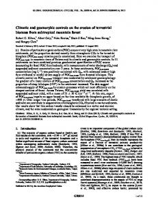
where ri are the residuals between measured and predicted quantities (PDZ thickness and surface elevation) and σ is the standard deviation of measured values. During each iteration an erosion history is used to drive the simulation. If the MLE for the simulation is greater than for the pervious iteration, the new erosion history is ‘accepted’ and slightly modified to drive the following iteration. If the MLE for the iteration is less than the previous iteration, it is accepted with a probability equal to the ratio between the two iterations. If the new history is ‘rejected’, then the subsequent iteration uses an erosion history slightly modified from the last accepted erosion history12. This method allows identification of the most likely erosion history at a field site given topographic and soil thickness data. 4. Example from Tennessee Valley, CA We have used geomorphic information to constrain particle ages at a site in Tennessee Valley, CA, where soil production and transport rates have been previously constrained4,11. We use a particle-based model2 to predict OSL ages in the soil and constrain the mixing velocity with measured OSL ages (Fig. 1a). We also constrain the history of erosion using measured topography and soil thickness (Fig. 1b). Because erosion rejuvenates hillslope topography, we are only able to resolve the last ~500kyr of erosion rates at the site (Fig. 1b).
Fig. 1.Using field data to reconstruct mixing and erosion rates at a field site in Tennessee Valley, CA. a. Mixing velocities constrained using a particle based model that compares predicted OSL ages against measured ages. b. Reconstruction of erosion history of the transect (negative values indicate deposition) based on a Monte Carlo Markov Chain analysis
These mixing and erosion parameters are used to drive a particle based weathering model2. We examine the hypothesis that primary rock forming minerals weather as a function of the time they spend in the weathering zone13. The concentrations of primary rock forming minerals at the field site were determined by quantitative XRF14. We simulated the predicted solid state geochemistry under several particle size scenarios (Fig 2). We find that in pits near the divide, the model is able to reproduce the enrichment of zirconium, which is frequently used as a weathering tracer5, measured in the PDZ if particles are assumed to be of silt size. The measured soil texture at the site is approximately 1/3 each of sand, silt and clay. The hillslope transect features thin PDZ (~30-35 cm thickness) from 0-~30 meters from the ridgetop and we have interpreted these soils to be responding to rapid erosion rates that occurred over the last ~300 kyrs (Fig 1b). Beyond 30m from the ridgetop, the hillslope transitions to a PDZ of >80 cm thickness, which the MCMC model suggests is due to increased deposition over the last