Appears in the Proceedings of the 15th Symposium on Parallelism in Algorithms and Architectures San Diego, CA, June 7-9, 2003
Quantifying Instruction Criticality for Shared Memory Multiprocessors Tong Li and Alvin R. Lebeck
Daniel J. Sorin
Department of Computer Science Duke University Durham, NC 27708, USA
Department of Electrical and Computer Engineering Duke University Durham, NC 27708, USA
{tongli,alvy}@cs.duke.edu
[email protected]
ABSTRACT
instruction-first). Recent research [3, 4, 12, 13, 14] advocates designing policies based on the criticality of dynamic instructions with respect to overall program performance. To quantify the criticality of dynamic instructions, Fields et al. [3, 4] propose a directed acyclic graph (DAG) model for characterizing the fine-grain microexecution of a sequential program. With this model, they can perform critical path analysis and quantify instruction criticality by using a dynamic instruction’s global slack value, where global slack is the amount the hardware can delay an instruction without lengthening the critical path of the execution. While prior research has demonstrated that instruction criticality is an effective metric for uniprocessors, this paper is the first research to extend the fine-grain criticality model and analysis to shared memory multiprocessors.
Recent research on processor microarchitecture suggests using instruction criticality as a metric to guide hardware control policies. Fields et al. [3, 4] have proposed a directed acyclic graph (DAG) model for characterizing program microexecutions on uniprocessors. Under such a model, critical path analysis can be applied and instructions’ slack values can be used to quantify instruction criticality. In this paper, we extend the uniprocessor DAG model to characterize parallel program executions on shared memory multiprocessor systems. We describe how critical path analysis can be applied, at a fine grain, in a multiprocessor system running both finite and continuous workloads. We provide detailed evaluations for various aspects of multiprocessor executions under the DAG model. To enable efficient offline critical path analysis, we propose a novel graph reduction technique that reduces a DAG to an equivalent but significantly smaller DAG.
Criticality-based control policies require that the hardware evaluate instruction criticality—either on a per-instruction basis or aggregated over intervals—on the fly and make decisions accordingly during program execution. Provided that such capabilities are available, the following list shows some potential advantages of criticality-based policies in a multiprocessor system.
Categories and Subject Descriptors C.1.2 [Processor Architectures]: Architectures (Multiprocessors)
Multiple
Data
Stream
•
Resource utilization. Resources (e.g., caches, memory bandwidth, network bandwidth) can be better utilized by prioritizing allocations and accesses based on instruction criticality.
•
Power efficiency. Processors executing less critical instructions can run more slowly, thus saving power without sacrificing performance.
•
Misspeculation reduction. Selectively applying speculation techniques based on instruction criticality can reduce the number of misspeculations. For instance, using coherence prediction to accelerate less critical instructions does not help improve overall performance even if the prediction is correct.
•
Dynamic scheduling. Multiprocessor systems typically perform dynamic scheduling at the task level to obtain an efficient schedule. With instruction criticality, it is possible to incorporate such fine-grain information with the scheduling algorithm to achieve a better schedule.
General Terms Algorithms, Measurement, Performance, Design
Keywords Shared memory multiprocessors, critical path analysis, slack
1. INTRODUCTION Computer hardware frequently makes decisions about how to manage its resources. For example, dynamically scheduled (a.k.a., out-of-order) superscalar microprocessors must decide how to schedule instructions and how to share resources (e.g., functional units or fetch bandwidth) among them. Until recently, microprocessors considered all instructions to have equal effect on performance, and they employed microarchitectural control policies (e.g., instruction issue policy) based on simple priority functions (e.g., oldest-
Before we can achieve these benefits of criticality-based policies, we must first extend the fine-grain uniprocessor DAG model and critical path analysis to multiprocessors. Specifically, we focus on modeling parallel program executions on shared-memory multiprocessor systems. We explore the graph properties of the resulting multiprocessor DAGs using offline analysis of traces of program executions. Previous multiprocessor DAG models represented programs at a coarse grain, such that each node in a DAG represented a
Permission to make digital or hard copies of all or part of this work for personal or classroom use is granted without fee provided that copies are not made or distributed for profit or commercial advantage and that copies bear this notice and the full citation on the first page. To copy otherwise, or republish, to post on servers or to redistribute to lists, requires prior specific permission and/or a fee. SPAA’03, June 7-9, 2003, San Diego, California, USA. Copyright 2003 ACM 1-58113-661-7/03/0006…$5.00.
1
task [8, 9] or a procedure [6, 7, 16]. In our fine-grain model, as in prior microprocessor work, each node represents the microexecution of an instruction. We seek to provide insights into the fine-grain instruction-level modeling of multiprocessor executions, so that we can exploit instruction criticality in system policies.
2
The remainder of this paper is organized as follows. In Section 2, we describe a general DAG model for program execution. Section 3 shows how to apply the model to represent uniprocessor executions and how we extend it to shared memory multiprocessors. Section 4 formalizes the definitions of local and global slack and presents an algorithm for computing them. The offline approach of our analysis requires significant storage space for keeping dynamic information during program executions. To ease this problem, we develop a graph reduction technique in Section 5. The graph reduction removes certain nodes and edges from a DAG without affecting the critical path and slack computation. In Section 6, we present experimental results on global slack distribution and show how the critical path spans across processors in a system. We then evaluate design decisions, such as the effects of different cache coherence protocols, and we present results on the effectiveness of the DAG reduction technique. We discuss related work in Section 7 and conclude in Section 8.
3
2
3
6
4
5
8
Figure 1. A simple DAG with critical path highlighted. The slack of an event is a measure of how long its start time can be delayed without affecting subsequent events. To distinguish types of slack, Fields et al. [3] introduce the concepts of local and global slack. In the DAG model, the local slack of a node is the maximum time the start of the corresponding event can be delayed without delaying any event in the descendent nodes.2 The global slack of a node is the maximum time the start of the event can be delayed without extending the DAG’s critical path. By definition, instructions on the critical path have both local and global slack of zero.
2. A DAG MODEL FOR EXECUTION We can model the execution of a program with a directed acyclic graph (DAG), in which each node represents a dynamic event of the program and each edge represents a dependence between its source and sink nodes. In this model, a dynamic event is a general term that can represent any event in the program’s execution (e.g., fetching an instruction, the execution of an entire instruction, or execution of a coarsegrain task). A dependence edge models the precedence constraints dictated by the program’s semantics (e.g., data dependence) or the underlying hardware (e.g., resource dependence). Each edge is weighted by the time required to resolve the corresponding dependence during the execution. For an edge e = (u, v), we say that e arrives at node v with arrival time t, where t is the time that the corresponding dependence is resolved. The arrival time of an edge is the real time during program execution (i.e., arrival times increase monotonically as the execution progresses). Among all edges arriving at v, we call the one that arrives last the last-arriving edge [4]. There can be more than one last-arriving edge when multiple edges arrive simultaneously.
3. MAPPING DAGS TO SYSTEMS In this section, we discuss how to map the DAG model to specific hardware systems.
3.1 Uniprocessor Systems Fields et al. [3, 4] model the execution of a single-threaded sequential program on a dynamically scheduled superscalar processor. In their DAG model, a node represents one of three events: instruction dispatch, execute, and commit. Each event corresponds to a stage in an instruction’s microexecution. An edge represents one of seven types of dependences.
A critical path of a DAG is a longest weighted path in the DAG. The events on a critical path determine the overall runtime of the program. If an edge e = (u, v) is on a DAG’s critical path, an important property is that e must be a lastarriving edge sinking on node v. Conversely, if an edge is not a last-arriving edge to its sink node, it must not be on a critical path. Note that a node with multiple last-arriving edges may possibly lead the DAG to have multiple critical paths.1 For the purposes of our critical path analysis, we do not explicitly label each edge with its weight; instead, we label each edge with the time that it arrives at the sink node. Figure 1 shows a simple DAG with its critical path highlighted. 1
4
(1) In-order dispatch: Instructions must be dispatched in the order in which they appear in the program. (2) Finite reorder buffer: When the reorder buffer is full, an instruction can be dispatched to it only after another instruction commits and frees an entry. (3) Control dependence: The correct target instruction of a mis-predicted branch cannot be dispatched until the branch is resolved. (4) Execution follows dispatch: An instruction cannot execute until it has been dispatched.
For brevity of terminology, we will refer without loss of generality to the critical path as encompassing these potentially multiple critical paths.
2
2
Node u is a descendent of v if there exists a path from u to v.
(5) Data dependence: An instruction cannot execute until the instructions producing its operands finish.
Processor 1
Processor 2
(6) Commit follows execution: An instruction cannot commit until it has finished execution.
Processor 3
Store
(7) In-order commit: Instructions must be committed in the order in which they appear in the program.
1
Types (1) and (7) collectively model the program order dependence required by the program's sequential semantics. The other dependence types reflect microarchitectural constraints that exist in most dynamically scheduled microprocessors.
2
3.2 Multiprocessor Systems
Load
4
2 3 Load
3
We extend the uniprocessor DAG model to parallel programs on shared memory multiprocessors. We first construct uniprocessor DAGs for each processor in the system, and then we add edges between them that correspond to inter-processor communication. Unlike prior work, to simplify the exposition, we consider multiprocessor systems with simple in-order processors (i.e., instructions dispatch, execute, and commit all in the order specified by the program). Since program order dictates the ordering of all dynamic instruction events, each node in our model represents an entire instruction (i.e., we do not split it into dispatch, execute, and commit). Within each processor, we maintain the program order dependence of its dynamic instructions. The only difference introduced by a dynamically scheduled processor model is the mapping of events and dependences to nodes and edges; the critical path analysis is the same.
7
5
4 Store
6
Load
Figure 2. A multiprocessor DAG (critical path highlighted).
4. COMPUTING SLACK In this section, we formally define local and global slack with respect to nodes and edges in a DAG (Section 4.1). We then present our algorithm for computing the global slack of all the nodes in a DAG (Section 4.2). While our algorithm computes the global slack, it can also determine the critical path of the DAG. Finally, we discuss how we apply the algorithm differently to finite and continuous workloads (Section 4.3).
In our model, a program order dependence edge connects an instruction to the instruction that immediately follows it in program order. The program order dependence resolves when the following instruction is issued to a functional unit for execution. Therefore, by the definition of the DAG model, we label a program order dependence edge with the issue time of the following instruction.
4.1 Definitions We use the global slack of an instruction to quantify its criticality. To compute global slack in a DAG, we use the same definitions developed by Fields et al. [3]. We present them again here in order to later explain our algorithm and reduction methodology.
Processors communicate with each other only via loads and stores to shared memory. Between instructions on different processors, true data dependence governs their ordering for the correctness of the program. Thus the other type of dependence we model, which does not exist in the uniprocessor model, is the read-after-write (RAW) dependence. A RAW dependence occurs between a store that produces a value and a load that consumes the value. When the store and load are on the same processor, the RAW edge connecting them models a normal data dependence as in the uniprocessor model. When the store and load are on different processors, the RAW edge models a communication between the two processors. A RAW dependence resolves when the store finishes. Therefore, we label a RAW edge with the store’s completion time.
Definition 1. The local slack of an edge e = (u, v), denoted by L(e), is the time that the latency of e can be increased without delaying the sink node v. We compute L(e) as the difference between the arrival time of the last-arriving edge sinking on node v and the arrival time of e. If e is last-arriving, L(e) = 0. Definition 2. The local slack of a node u, denoted by L(u), is the maximum time u can be delayed without delaying any of its descendent nodes. We compute L(u) as the smallest local slack among the outgoing edges of u, i.e., L(u) = mini(L(ei)), where ei is the ith outgoing edge of node u.
Since we model only two types of dependences, a node in our DAG model has at most two incoming edges: a program order edge and a RAW edge. Only load nodes have incoming RAW edges and only store nodes have outgoing RAW edges. Figure 2 shows an example DAG for a multiprocessor system with its critical path highlighted. Unlabeled nodes are instructions that are neither loads nor stores.
Definition 3. The global slack of an edge e = (u, v), denoted by G(e), is the time that the latency of e can be increased without extending the critical path. We compute G(e) as L(e) + mini(G(oi)), where oi is the ith outgoing edge of the sink node v.
3
Algorithm 1: Computing global slack for all nodes.
G(u)
if u is the endpoint node then
u
G(u) = 0 else if u has no outgoing edges then
L(e n)
L(e1)
G(u) = finish_time(endpoint) - finish_time(u)
L(e 2)
else G(u) = undefined
v1
v2
G(v1 )
G(v2)
...
...
end if
vn
Sort all nodes in reverse topological order
G(vn)
for all nodes u in the sorted order do if G(u) = undefined then
Figure 3. Computing the global slack of node u.
min_global_slack = infinity for all of u’s outgoing edges ei = (u, vi) do compute L(ei)
Definition 4. The global slack of a node u, denoted by G(u), is the maximum time u can be delayed without extending the critical path of the DAG.
if L(ei) + G(vi) < min_global_slack then min_global_slack = L(ei) + G(vi)
We compute G(u) as the smallest global slack among the outgoing edges of u, i.e., G(u) = mini(G(ei)), where ei is the ith outgoing edge of node u.
end if end for G(u) = min_global_slack
Given these definitions, we can derive G(u) from u’s outgoing edges and the global slack of their sink nodes.
end if
Let u be a node, ei = (u, vi) be the ith outgoing edge of node u, and oij be the jth outgoing edge of sink node vi. We have
end for properties of a DAG; therefore we can apply it directly to DAGs modeling dynamically scheduled processors.
G ( u ) = min ( G ( e i ) ) i = min ( L ( e i ) + min ( G ( o ij ) ) ) i j = min ( L ( e i ) + G ( v i ) ) . i
4.3 Finite vs. Continuous Workloads
(EQ 1)
A finite workload, such as a scientific application, executes a finite number of instructions, so we can construct a DAG for all its dynamic instructions that has a well-defined endpoint. However, a continuous workload, such as a web server or database, executes continuously and thus does not have a welldefined endpoint. Nevertheless, given a large interval of execution, we can pick the last finished node within the interval from an arbitrary processor and consider it to be the endpoint. We construct a DAG that includes only the finite number of instructions that directly or transitively lead to the endpoint node via program order and/or RAW dependence edges. If a DAG node has an outgoing dependence edge to a node outside the DAG, we do not include this edge in the DAG. Unlike DAGs for finite workloads, in which nonendpoint nodes can have no outgoing edges, the endpoint node in a continuous workload DAG is the only node that has no outgoing edges. A DAG constructed in this way allows us to apply our algorithm to a finite subset of the infinitely many instructions in a continuous workload, and it enables control policies to apply optimizations to these instructions without increasing their overall runtime. Randomly choosing the endpoint node from all the processors affects the individual instruction slack values computed by the algorithm. Nevertheless, as shown in Section 6.2, the endpoint choice has negligible impact on the overall slack distribution among the instructions. This result suggests that we can design more sophisticated control policies based on aggregated slack values over an interval.
We illustrate this computation in Figure 3, and we note that it lends itself to an algorithm that starts at the end of execution and proceeds backwards in time.
4.2 Algorithm for Computing Global Slack Equation 1 shows a recursive way to compute the global slack of all nodes in a DAG. We now define the base case for the recursion. We define the endpoint node of a DAG as the last finished node (instruction) among all the nodes in the DAG. When there are multiple last finished nodes (because they finish at the same time on different processors), we choose an arbitrary node among them to be the endpoint node. We initialize the global slack of the endpoint node to zero. If a non-endpoint node has no descendents (i.e., it has no outgoing edges) in the DAG, we initialize its global slack to be the difference between its finish time and the finish time of the endpoint node. During program execution, we store information about its instructions so that we can construct the DAG for offline processing. Algorithm 1 shows how we compute the global slack for all the nodes in a DAG. Since instructions on the critical path have global slack of zero, we can determine the critical path by backtracing the DAG from its endpoint node. On the backtrace, all nodes with global slack of zero constitute the critical path. Our algorithm does not assume any special
4
G(vj). Since e is the only edge sinking on vj, by definition, L(e) = 0. Therefore, G(vi) = G(vj). Let e’ be the program order edge connecting nodes vk-1 and vk. Inductively, we have
v0
.. .
G ( v 1 ) = G ( v 2 ) = … = G ( v k – 1 ) = L ( e' ) + G ( v k ).
vi
Since we compute L(e’) by using the arrival times of the edges sinking on vk, and we compute G(vk) by using vk’s outgoing edges and descendent nodes, which are all retained in the reduced DAG, we can correctly derive the global slack of nodes v1, ... , vk-1 if they are removed. 3
v0
e Reduction arrival time = t
vj
.. .
We can also derive the critical path from the reduced DAG. If the removed nodes are on the critical path of the original DAG, then vk must be on the critical path and e’ must be a lastarriving edge to vk. Since the arrival time of e’ is retained in the reduced graph, we must find that both v0 and vk are on the critical path in the reduced DAG, and from this we can derive that all the removed intermediate nodes must also be on the critical path in the original DAG. Conversely, if the removed nodes are not on the critical path of the original DAG, then we know either vk is not on the critical path of the original DAG, or, if it is, e’ must not be a last-arriving edge to vk. For either case, we must not find in the reduced DAG that both v0 and vk appear on the critical path at the same time. Therefore we can derive that the removed nodes are not on the critical path of the original DAG. ❏
vk
vk-1
e’
arrival time = t vk Figure 4. Illustration for Theorem 1.
Since only load and store nodes have RAW edges, by Theorem 1, we can remove all the other nodes without changing the critical path and slack information. We retain, however, all the nodes that do not have outgoing edges since they are part of the base case of our algorithm. 4 Other than these nodes, with the reduction, a DAG now contains only load and store nodes and the edges connecting them.
5. GRAPH REDUCTION The algorithm described in the previous section assumes that we have enough information to construct the DAG for a given program’s execution. In our model, a DAG contains nodes representing all dynamic instructions, which can be a large amount of information to store. For example, the sizes of our workloads running with eight processors are all on the order of billions of instructions. Though not infeasible, it is certainly non-scalable and time-consuming to store and process such a large amount of information. To ease this problem, we developed a reduction technique that reduces a DAG to a much smaller one without changing its critical path and slack properties. The reduction exploits the observation that many nodes and edges are not “useful” for computing the critical path of the DAG or the global slack of any node in the DAG, and thus they can be removed from the DAG.
Definition 6. Given a DAG G, a RAW edge e = (u, v) is dominated if removing it from G produces a DAG that is equivalent to G. The rest of the reduction is based on the observation that many RAW edges are dominated and thus can be removed from the DAG. The following lemma states the conditions for a RAW edge to be dominated. Lemma 1. Given a DAG G, a RAW edge e = (u, v) is dominated if it does not contribute to the computation of any of the following values:
Definition 5. DAG A is equivalent to DAG B if an algorithm can derive from A the critical path of B and the global slack of each node in B.
(i)
the critical path of G,
(ii) the global slack of node u, and
There are three cases in which the reduction can be applied. We describe them as three theorems and show proofs for their correctness.
(iii) the local slack of the program order edge into node v. Proof. Since the RAW edge e does not contribute to the computation of the critical path of G, removing it from G does not change the critical path.
Theorem 1. Let v0 and vk be two nodes on the same processor, and let p = (v0, v1, ... , vk-1, vk) be the path connecting them via only program order edges. If all the intermediate nodes on p (i.e., nodes v1, ... , vk-1) have neither incoming nor outgoing RAW edges, then we can reduce the DAG to an equivalent DAG by removing all the intermediate nodes and connecting v0 and vk directly with an edge labeled with the same arrival time as that of the original program order edge sinking on vk.
Let e’ = (w, v) be the program order edge sinking on v. By definition, the RAW edge e is only useful for computing the global slack of u and w, and e affects G(w) only if it contributes to the computation of L(e’). Given the conditions 3
Depending on how the slack information is to be used, we may optionally store in vk the number of nodes that are removed so we can accurately derive how many nodes were present in the original DAG. 4 In a continuous workload, the chosen endpoint node is the only node that does not have outgoing edges.
Proof. Figure 4 shows the situation described by the theorem. Let vi and vj be two arbitrary intermediate nodes on the path p, and let e be the program order edge connecting them. Since e is the only outgoing edge from vi, by Equation 1, G(vi) = L(e) +
5
u
e’
pw
u e’
w w e
e
pv v
v Figure 5. Illustration for Theorem 2.
Figure 6. Illustration for Theorem 3.
in the lemma, removing e does not change the global slack of any node in the DAG.
Now consider the global slack of u. We have G(u) = min(L(e) + G(v), L(e’) + G(w)). Edges e and e’ have the same arrival time at their corresponding sink nodes (both edges are labeled with node u’s completion time), and because w is earlier than v in program order, the arrival time of pw is less than that of pv. Therefore L(e’) < L(e). Since we know that G(w) ≤ G(v), we have G(u) = L(e’) + G(w). Therefore, removing e does not affect the computation of the global slack of u. ❏
Therefore, removing e from G produces a DAG that is equivalent to G. By definition, the edge e is dominated. ❏ Given Lemma 1, we can prove two sufficient conditions for a RAW edge to be dominated. The first condition considers the case in which a store has two consuming loads that are performed by the same processor.
The first three conditions in Theorem 2 describe a situation that occurs frequently in a program. A value stored by an instruction is read repeatedly by later loads on the same or different processor after the store has already finished. Thus, if the last condition in the theorem is also satisfied, we can remove all such later RAW edges (except the first one) from the DAG.
Theorem 2. A RAW edge e = (u, v) is dominated if there exists another edge e’ = (u, w) such that (i)
nodes w and v are on the same processor;
(ii) node w appears before v in program order; (iii) the arrival time of e is less than that of the program order edge sinking on v; and
Theorem 2 considers the situation in which a sequence of RAW edges can be removed except for the first one in the sequence. In the following theorem, we consider a situation in which the RAW edge of the first instruction that loads a value can be removed.
(iv) no node between w and v is the sink of a RAW edge whose arrival time is greater than that of the program order edge sinking on that node. Proof. Figure 5 shows the situation described by the theorem. Dashed lines are program order edges and solid lines are RAW edges. Let pw and pv denote the program order edges sinking on w and v, respectively.
Theorem 3. A RAW edge e = (u, v) is dominated if (i)
nodes u and v are on the same processor;
(ii) the arrival time of e is less than that of the program order edge sinking on v; and
To show that edge e is dominated, we prove that e does not contribute to the computation of any of the three values listed in Lemma 1.
(iii) no node between u and v is the sink of a RAW edge whose arrival time is greater than that of the program order edge sinking on that node.
First, by condition (iii), pv is the last-arriving edge to the node v. Therefore edge e must not be on the critical path, i.e., removing e does not affect the computation of the critical path. Second, since pv is the last-arriving edge to v, by definition, the local slack of pv, L(pv), is zero. Thus, removing e does not affect the computation of L(pv).
Proof. Figure 6 shows the situation described by the theorem. Conditions (i) and (ii) ensure that e does not contribute to the computation of the critical path and the local slack of the program order edge sinking on v.
Third, we prove that e does not contribute to the computation of the global slack of node u. Consider the path from w to v. Let n1, ... , nk be the intermediate nodes on the path. From condition (iv), we know that for every intermediate node, its incoming program order edge is the last-arriving edge, which has local slack zero. Therefore, we have G(w) ≤ G(n1) ≤ ... ≤ G(nk) ≤ G(v).
Let e’ be the program order edge out of u and let w be the sink node of e’. From Condition (iii), we know that e’ is the lastarriving edge to w. Thus we have L(e’) = 0 ≤ L(e). Similar to Theorem 2, Condition (iii) also ensures that G(w) ≤ G(v). Therefore G(u) = min(L(e) + G(v), L(e’) + G(w)) = L(e’) + G(w). This proves that e does not contribute to the computation of the global slack of u. ❏
6
Conditions (i) and (ii) in Theorem 3 describe the frequent situation in which a store writes a value and has already finished by the time a later load is issued to read the value.
Table 1. Target system parameters.
The three theorems described in this section allow us to reduce a DAG to an equivalent but much smaller DAG. Moreover, we can apply these theorems repeatedly. For example, after removing the RAW edges by Theorems 2 and 3, we may further reduce the DAG by applying Theorem 1. In Section 6, we evaluate the effectiveness of the reduction. These reduction theorems were derived for systems with in-order processors. DAGs for dynamically scheduled processor models may require different graph reduction theorems.
L1 Cache (I and D)
128 KB, 4-way set associative
L2 Cache
4 MB, 4-way set-associative
Memory
2 GB, 64 byte blocks
Miss From Memory
180 ns (uncontended)
Network
tree, link b/w = 6.4 GB/sec
changes required for a dynamically scheduled processor model involve the mapping of events and dependences to the DAG.
6. EXPERIMENTAL RESULTS
Memory Model. We have implemented a memory hierarchy simulator that supports a MOSI broadcast snooping cache coherence protocol. The simulator captures all state transitions (including transient states) of our coherence protocol in the cache and memory controllers. Our memory model is sequential consistency and we model the interconnection network and the contention within it. In Table 1, we present the design parameters of our target memory system.
In this section, we describe our simulation methodology and present detailed evaluations for various aspects of program executions under our multiprocessor DAG model.
6.1 Methodology We simulate a multiprocessor target system with the Simics full-system, multiprocessor, functional simulator [10], and we extend Simics with a memory hierarchy simulator to compute execution times. Each node in our system consists of a processor, two levels of cache, some portion of the shared memory, and a network interface.
Workloads. We evaluate our system with the four continuous commercial applications of the Wisconsin Commercial Workload Suite [1] and two finite scientific applications. These workloads are described briefly in Table 2 and in more detail by Alameldeen et al. [1].
Simics. Simics is a system-level architectural simulator developed by Virtutech AB. We use Simics/sun4u, which simulates Sun Microsystems’ SPARC V9 platform architecture (e.g., used for Sun E6000s) in sufficient detail to boot unmodified Solaris 8. Simics is a functional simulator only, and it assumes that each instruction takes one cycle to execute (although I/O may take longer), but it provides an interface to support detailed memory hierarchy simulation.
Data Collection. Our simulator assigns a sequence number to each dynamic instruction when the instruction is issued for execution. The sequence number is a unique, monotonically increasing integer across all instructions on the same processor. A (processor ID, sequence number) pair thus uniquely identifies an instruction in the system. During execution, the simulator tracks instruction dependences and stores them in a file. Each line of the file contains information that uniquely identifies an edge in the program’s DAG. For each edge, we store the (processor ID, sequence number) pair, the issue time, and the completion time of both its source and sink nodes. We store only RAW edges, since we can derive program order edges by the sequence numbers of the nodes stored in the file. To ensure that we store only necessary
Processor Model. We use Simics to model a processor core that, given a perfect memory system, would execute four billion instructions per second and generate blocking requests to the cache hierarchy and beyond. We use this simple processor model to enable tractable simulation times for fullsystem simulation of commercial workloads. Our critical path analysis, however, applies to any processor model. The only
Table 2. Workloads: Wisconsin Commercial Workload Suite [1] and two SPLASH-2 benchmarks. OLTP: Our OLTP workload is based on the TPC-C v3.0 benchmark using IBM’s DB2 v7.2 EEE database management system. We use a 1 GB 10-warehouse database stored on five raw disks and an additional dedicated database log disk. There are eight simulated users per processor. We warm up for 10,000 transactions, and we run for 500 transactions. Java Server: SPECjbb2000 is a server-side java benchmark that models a three-tier system with driver threads. We used Sun’s HotSpot 1.4.0 Server JVM. Our experiments use 24 threads and 24 warehouses (~500 MB of data). We warm up for 100,000 transactions, and we run for 50,000 transactions. Static Web Server: We use Apache 1.3.19 (www.apache.org) for SPARC/Solaris 8, configured to use pthread locks and minimal logging as the web server. We use SURGE to generate web requests. We use a repository of 2,000 files (totalling ~50 MB). There are ten simulated users per processor. We warm up for ~80,000 requests, and we run for 5,000 requests. Dynamic Web Server: Slashcode is based on a dynamic web message posting system used by slashdot.com. We use Slashcode 2.0, Apache 1.3.20, and Apache’s mod_perl 1.25 module for the web server. MySQL 3.23.39 is the database engine. The database is a snapshot of slashcode.com, and it contains ~3,000 messages. A multithreaded driver simulates browsing and posting behavior for three users per processor. We warm up for 240 transactions, and we run for 50 transactions. Scientific Applications: We use two benchmarks from the SPLASH-2 suite [15]. We use barnes-hut with the 64K body input set and ocean with the 514x514 input size. For both, we measure from the start of the parallel phase to avoid measuring thread forking.
7
oltp
oltp 0.12
8 Processors
2 Processors PDF: fraction of instructions with global slack = x
PDF: fraction of instructions with global slack = x
0.6 0.5 0.4 0.3 0.2 0.1
0.1 0.08 0.06 0.04 0.02 0
0 1
10
100 1000 GlobalSlack + 1
10000
1
100000
10
100
1000
10000
100000
GlobalSlack + 1
Figure 7. Multiprocessor slack distribution. processor system. We plot our results only for ocean and slash; for the other workloads, the critical path is almost evenly distributed with a maximum 7% variation across all the processors. These critical path time breakdowns closely correspond with the L2 cache miss rates on the processors, since a processor with a larger L2 cache miss rate incurs more communication to remote memories, thus taking a higher fraction of the critical path’s time. In ocean, processor 0 dominates the critical path, which is unsurprising since processor 0 performs the sequential work in this algorithm.
0.3
Fraction of CP time
0.25 0.2 ocean slash
0.15 0.1 0.05
Broadcast vs. Directory Protocols. To study how different cache coherence protocols affect the distribution of global slack, we compare our MOSI broadcast snooping protocol with a directory protocol similar to that used in the AlphaServer GS320 [5]. In Figure 9, we plot the cumulative distribution function (CDF) of global slack for apache and jbb on an 8processor system. The x-axis is the global slack value plus one shown in log scale. For any global slack x, the y-axis corresponds to the fraction of DAG nodes (instructions) that have global slack less than or equal to x. From the results, we see that instructions in the directory system possess more slack than those in the broadcast system. Since the systems we model have plentiful network bandwidth, by broadcasting cache block requests to all nodes in the system, the broadcast protocol avoids indirections and achieves better performance than the directory protocol. Our results show that, on average, the critical path of a workload in the directory system is 38% longer in time than that in the broadcast system. In the directory system, instructions typically wait longer for cache misses, thus making them have more slack in their executions.
0 0
1
2
3
4
5
6
7
Processor ID
Figure 8. Fraction of critical path’s time on each processor. information, the simulator dynamically checks whether it can apply a graph reduction.
6.2 Results In this section, we present our results on global slack distribution and how the critical path spans across the processors in a system. We then evaluate how different cache coherence protocols and the endpoint choice in a continuous workload affect the slack distribution. Finally we show results on the effectiveness of the graph reduction. Slack Distribution. In Figure 7, we plot the probability density function (PDF) of global slack for 2-processor and 8-processor OLTP workloads. The x-axis is global slack plus one shown in log scale, so as to provide more resolution for small values and allow the x-axis to represent zero global slack in log scale. The y-axis is the fraction of instructions that have the given global slack value specified by the x-axis. We observe that most instructions have global slack less than 100 ns. There are, however, spikes in the distributions between 100 and 200 ns, which correspond to the latency of inter-processor communication. The spike for the 4-processor workload (not shown) lies between these two. The results for the other workloads are similar.
Choice of Endpoint Processor. In Section 4.3, we claimed that, for continuous workloads, we can choose the last finished node from an arbitrary processor as the endpoint node. We now present results that support this claim. To investigate the effects of the endpoint choice, we ran Algorithm 1 for each of our continuous workloads (apache, jbb, oltp, and slash) P times for a system of P processors, and in each run we constructed a DAG with the endpoint node chosen from a different processor. Our results show that, for each workload, all of the P DAGs have almost identical global slack distribution. Specifically, for any given global slack x, the fraction of instructions that have global slack x differs on average by the order of 10-7 in their values among all P DAGs. Moreover, the fraction of instructions that are on the critical path (i.e., with global slack zero) differs on average by 10-4 in
Critical Path Time Breakdown. The breakdown of the critical path’s time on each processor provides insight into the relative criticality of the processors. In Figure 8, we show the fraction of the critical path’s time spent on each processor in an 8-
8
jbb 1
CDF: fraction of instructions with global slack