on the time-dependent wave-packet method, is presented in detail. In contrast to ... 6Li + 209Bi at energies around the Coulomb barrier demonstrate that converged reliable excitation ... jectile nucleus breaking up, at a given incident energy.
Quantifying low-energy fusion dynamics of weakly bound nuclei from a time-dependent quantum perspective Maddalena Boselli and Alexis Diaz-Torres European Centre for Theoretical Studies in Nuclear Physics and Related Areas (ECT∗ ), Strada delle Tabarelle 286, I-38123 Villazzano, Trento, Italy (Dated: September 30, 2015) A quantum reaction approach to low-energy collisions of weakly-bound few-body nuclei, based on the time-dependent wave-packet method, is presented in detail. In contrast to existing models that use this perspective, the approach separates the complete and incomplete fusion from the total fusion. Calculations performed within a one-dimensional model with two degrees of freedom for 6 Li + 209 Bi at energies around the Coulomb barrier demonstrate that converged reliable excitation functions for total, incomplete and complete fusion can be obtained with this type of approach. PACS numbers: 25.60.Pj, 25.60.-t, 24.10.-i
I.
INTRODUCTION
Nowadays many facilities are being built around the world to perform measurements using beams of exotic nuclei (often called RIB: Radioactive Ion Beams). Performing good measurements is laborious for various reasons, as the RIB needs to satisfy some basic properties: it is desirable for it to be intense, pure and able to cover a wide range of incident energies. This means that the production of such a beam has to be fast, selective, efficient and with a high production rate. Details about the techniques used to produce RIB can be found in [1]. Since producing a good quality RIB is extremely challenging, a theory able to describe the dynamics of these exotic nuclei could be helpful for better planning and interpretation of measurements. Investigating the reaction dynamics of low energy collisions involving a halo projectile nucleus is a challenging task, from the theoretical point of view as well as from the experimental one [2, 3]. A halo nucleus is typically weakly bound with a few-body cluster structure and its key feature is that it can be easily separated into its constituents. Because of the possibility of the projectile nucleus breaking up, at a given incident energy several reaction paths (or channels) are available simultaneously, as shown in Fig. 1. These can be grouped in two main categories: events where none of the projectile fragments are captured by the target, called nocapture break-up (NCBU), and events associated with the fusion process. Among these, we can further distinguish between the case where just part of the fragments are captured, incomplete fusion (ICF), and the case where the projectile is fully captured, complete fusion (CF). It can be observed in Fig. 1 that two different processes contribute to the complete fusion event: one where the projectile breaks up and all the fragments are captured, and one where the projectile fuses with the target without a preceding break up. One of the key points is to understand how the projectile’s break up, and thus its internal structure, are related with the different fusion processes. The difficulty lies in setting up a quantum
FIG. 1: (Color online) Some key reaction processes induced by a weakly-bound two-body nucleus at low incident energies.
theory able to describe and quantify (calculating observables) each process at the same time and independently one from the other. Among other reasons, theorists are interested in studying this kind of problems because low energy nuclear reactions involving halo nuclei occur during the nucleosynthesis of heavy elements (heavier than 56 Fe) in the rapid neutron-capture process. During the past years a lot of work has been done and several models of different nature (classical, quantum mechanical and also semiclassical) have been proposed. The continuum discretized coupled channels (CDCC) method [4] is one of those which provides good results concerning certain observables such as the total fusion (TF) (i.e., the sum of ICF and CF), the elastic and NCBU cross sections. But it has a strong limitation as it cannot calculate
TABLE I: Parameters of the Woods-Saxon nuclear potential, which are used for different binary systems in the present calculations, as well as the radius parameter of the uniformly charged sphere for their Coulomb interactions (last column). System
V0 (MeV) r0 (fm) a0 (fm) r0c (fm)
209
-50.000 -32.931 -26.000 -78.460
Bi-6 Li Bi-4 He 209 Bi-2 H 4 He + 2 H 209
A.
FIG. 2: (Color online) Illustration of the one-dimensional three-body model and its coordinates.
the integrated ICF and CF cross sections unambiguously. A classical model [5–7] overcomes some problems but, not being a quantum mechanical model, it does not include the quantum tunnelling probability. The aim of this article is to describe in detail a new type of approach [8] which tries to offer a solution to the limitations of the other previous models mentioned above. In Section 2, the theoretical concepts and associated formulae on which the method is based are presented within a simple model. Section 3 shows numerical results concerning the convergence of fusion excitation functions within the present approach. Since the model is schematic, the physical interpretation of its results is only qualitative. A summary is given in Section 4.
II.
METHODOLOGY
The present three-body model addresses the reaction problem from a time-dependent perspective, allowing to follow the time evolution of the reaction processes. It makes it possible to construct a picture of what is happening at any desired moment, facilitating the understanding of how the reaction observables emerge during the nuclear collision. This perspective has been already employed in the past, e.g., see Ref. [9]. The method consists of three main steps: (i) to compute the three body wave function, Ψ(t = 0), describing the system at the initial time, (ii) to propagate Ψ(0) → Ψ(t), where the propagation is governed by the time evolution operator, ˆ ˆ being the total Hamiltonian exp(−iHt/~), with H of the system, (iii) after a long propagation time, tf , to calculate energy-resolved observables using the wave function Ψ(tf ).
0.950 1.461 1.465 1.150
1.050 0.605 0.668 0.700
1.2 1.2 1.2 1.465
A simple model with two degrees of freedom
As a test case, we will study the 6 Li+209 Bi fusion within a one-dimensional model with two degrees of freedom, where the 209 Bi target and the 6 Li fragments (4 He and 2 H) are always on a line. Fig. 2 shows the coordinate system employed in the model (Jacobi coordinates for a system of three bodies), with the projectile considered as composed of two bodies (or fragments). Xc.m. identifies the distance between the target and the center of mass (c.m.) of the projectile, while ξ gives the distance between the projectile constituents. M is the mass of the target nucleus, while m1 and m2 are the masses of the projectile constituents. The Hamiltonian of the system in terms of these coordinates reads: ˆ = H
2 pˆ2ξ PˆX c.m. + + U12 (ξ) 2µT P 2µ12 +VT 1 (Xc.m. − α ξ) + VT 2 (Xc.m. + β ξ),
(1)
where µT P = M (m1 + m2 )/(M + m1 + m2 ), µ12 = m1 m2 /(m1 + m2 ), α = m2 /(m1 + m2 ), β = m1 /(m1 + m2 ). U12 represents the interaction between the fragments. VT 1 and VT 2 describe the interaction between target and the two projectile fragments, respectively, which depend on the relative distances x1 = Xc.m. − α ξ and x2 = Xc.m. + β ξ, as shown in Fig. 2. Table I presents the parameters of the Woods-Saxon nuclear potential for the binary systems in the calculations below, while for their Coulomb interaction the potential of a uniformly charged sphere has been used. Please note that all the radius parameters provide a critical distance determined by r0 A1/3 , where A is the heaviest mass in the corresponding binary system. The Coulomb barriers between the projectile fragments and the target obtained with these potentials are as follows: (VB , RB ) = (21.25 MeV, 10.55 fm) for 4 He+209 Bi and (10.08 MeV, 11.12 fm) for 2 H+209 Bi. These values are similar to the Sao-Paulo potential barriers [10]. To describe fusion of the projectile fragments with the target, which is an irreversible process, the Hamiltonian in Eq. (1) is augmented with two strong imaginary potentials, iWT 1 (x1 ) and iWT 2 (x2 ), which operate in the interior of the individual Coulomb barriers between the target and the projectile fragments. This is usually employed in coupled-channels model to simulate
1.
Initial wave function
Since at the initial time the projectile is considered to be far away from the target, VT 1 and VT 2 in Eq. (1) can be neglected and the Hamiltonian becomes separable. Consequently, the initial wave function can be factorized as Ψ(ξ, Xc.m. , t = 0) = Φ0 (Xc.m. ) χ0 (ξ),
g.s. probability density
fusion and is equivalent to the use of the ingoing-wave boundary condition (IWBC) [4, 11]. The imaginary potentials have the same Woods-Saxon shape: (W0 , a0w ) = (−50.0 MeV, 0.1 fm), centered at the minimum of the individual potential pockets.
0.4 6
0.3 0.2
(a) 0.1 0 0
10
˜ n (ξ) = En χn (ξ), Hχ
8
Φ0 (Xc.m. ) =
1 √ e π 1/4 σ
e−iK0 (Xc.m. −X0 ) .
Time propagation
The formal solution of the time-dependent Schr¨odinger equation at time t + ∆t reads: ˆ ∆t � H Ψ(t + ∆t) = exp − i Ψ(t). ~ �
(5)
The time evolution operator is represented as a convergent series of polynomials Qn (see Ref. [12]): � X ˆ ∆t � H ˆ norm ). ≈ an Qn (H exp − i ~ n
(6)
6
8
(b) ξ (fm)
(3)
(4) Figure 3 (a) shows the probability density of the groundstate wave function of a pseudo-6 Li projectile (= 4 He + 2 H). This wave function is calculated using a nuclear Woods-Saxon potential between the alpha particle and the deuteron, shown in Table I, which provides a 1sstate with a separation energy of −1.47 MeV. It is assumed that the strongly bound 0s-state (−32.96 MeV) is occupied by the 4 He nucleons. As an example, Fig. 3 (b) shows a map of probability associated with Eq. (2), where X0 = 50 fm and σ = 10 fm. Please note that the Xc.m. and ξ coordinates are strongly coupled when the 6 Li and 209 Bi nuclei come together, so a product state like Eq. (2) is only justified asymptotically. 2.
4
10
ξ (fm)
where χ0 describes the ground state of the projectile and it is determined by solving the eigenvalue problem
(X −X0 )2 − c.m. 2σ2
2
(2)
˜ being the part of the Hamiltonian in Eq. (1) with H which contains the dependency only on ξ, and keeping the eigenfunction associated with the physically motivated smallest eigenvalue. Concerning Φ0 (Xc.m. ), it is chosen to be a Gaussian wave-packet centered in X0 , with spatial width σ and average wave-number K0 :
Li
10
-3
10
-4
10
-5
2 0
10
-6
6 4
40 50 60 Xc.m. (fm) FIG. 3: (Color online) (a) The density of probability of the 6 Li ground-state wave function, and (b) the initial map of probability which includes the initial wave-packet describing the 209 Bi-6 Li relative motion.
In Eq.(6), the time-independent Hamiltonian is renormalized so that its spectral range is within the interval [-1,1], which is the domain of the polynomials, by defining ¯ˆ ˆ ˆ norm = (H 1 − H) , H ∆H
(7)
¯ = (λmax + λmin )/2, ∆H = (λmax − λmin )/2, where H λmax and λmin are respectively the largest and smallest ˆ supported by the nueigenvalues in the spectrum of H ˆ merical grid, and 1 denotes the identity operator. The expansion coefficients in Eq.(6) read: an = in (2 − δn0 ) exp(−i
¯ ∆t H ∆H ∆t ) Jn ( ), ~ ~
(8)
where Jn are Bessel functions of the first kind. Since Jn (x) exponentially goes to zero with increasing n for n > x, the expansion in Eq.(6) converges exponentially for n > ∆H∆t/~. This representation of the time evolution operator reˆ norm ) on quires the computation of the action of Qn (H
the wave function Ψ(t). The Qn polynomials obey the recurrence relations [12]: ˆ norm ) + e Qn+1 (H ˆ norm ) Qn−1 (H ˆ ˆ −2Hnorm Qn (Hnorm ) = 0,
-22
t = 13 x 10
γ ˆ
(9)
ˆ norm ) = ˆ1 and with the initial conditions Q0 (H −ˆ γ ˆ ˆ Q1 (Hnorm ) = e Hnorm . Here, γˆ is an operator, function of (ξ, Xc.m. ), related to the optical potential ˆ (ξ, Xc.m. ). As explained above, in order to simulate W the irreversibility of the fusion process, two imaginary ˆ T 1 (x1 ) and W ˆ T 2 (x2 ) are added to the Hamilpotentials W tonian. Following Ref. [12], these are given by:
ξ (fm)
e
−ˆ γ
30 25 20 15 10 5 0
s
(a)
0
5
10
15
10
-4
10
-6
10
-8
10
-10
10
-2
10
-4
10
-6
10
-8
20
Xc.m. (fm)
ˆ T j = ∆H [cos δ (1 − cosh γˆj ) − i sin δ sinh γˆj ], (10) W ¯
ˆ T 1 (x1 ) + W ˆ T 2 (x2 ) = W ˆ (ξ, Xc.m. ) W From Eq.(10) and Eq.(11) it follows that: � � sinh(ˆ γ1 ) + sinh(ˆ γ2 ) −1 γˆ = tanh cosh(ˆ γ1 ) + cosh(ˆ γ2 ) − 1
-22
t = 20 x 10
ξ (fm)
H where δ = arcos ( E− ∆H ), E denotes the incident energy and j = 1, 2 identifies the projectile fragment. Since the time-dependent Schr¨odinger equation is represented in terms of the Jacobi coordinates, the absorbing potential also needs to be represented in those coordinates. The relationship between the total absorbing potential as a function of the coordinates (x1 , x2 ) and that in terms of (ξ, Xc.m. ) reads:
(11)
30 25 20 15 10 5 0
(b)
0
5
10
15
20
Xc.m. (fm)
(12)
where the operators γˆ1 (x1 ) and γˆ2 (x2 ) result from Eq. (10), thus γˆ = γˆ (ξ, Xc.m. ). The quantity e−ˆγ (ξ,Xc.m. ) in Eq.(9) acts like a damping factor for the wave function: in case of no absorption ˆ j = 0 implies γˆj = 0), the factor e−ˆγ (ξ,Xc.m. ) = 1 and (W the Qn polynomials in Eq.(9) are the Chebyshev polynomials. The expansion in Eq.(6) corresponds to the standard Chebyshev propagator [13] and the wave function preserves its norm. On the other side, when the absorption is present, the quantity e−ˆγ (ξ,Xc.m. ) becomes smaller (tends to zero), the wave function is damped and its norm is no longer preserved. This mechanism simulates the fusion process when flux is removed from the entrance channel. In this work, ∆t = 10−22 s, and in absence of the imaginary potentials the norm of the wave function is preserved with an accuracy of ∼ 10−14 . Chapter 11 in Ref. [14] provides a survey of techniques for solving the time-dependent Schr¨odinger equation, which are distinguished by the numerical implementation of the time evolution operator in Eq. (5). As an example, Fig. (4) shows maps of probability associated with the time-propagating total wave function, at two times, when the main body of the wave-packet in Fig. 3 (b) is close to the interaction region. The moving region of maximal probability includes the contribution of the different wave-function components which are not
s
FIG. 4: (Color online) Maps of probability of the timedependent total wave function, when the main body of the wave-packet in Fig. 3 (b) is near the interaction region. The white region is innaccessible with the model, as all the coordinates in Fig. 2 are positive.
fully absorbed by the two imaginary potentials, such as the scattering and the ICF parts of the total wave function; all the contributions being summed up over a range of incident energies around the average energy of the initial wave packet.
3.
Energy-resolved fusion cross sections
In the present work, we concentrate on the TF, ICF and CF cross sections: σT F , σICF and σCF . A limitation of most fusion models of weakly bound nuclei is the lack of an unambiguous calculation of σICF and σCF [8]. The key idea to overcome this issue is to examine the location of each fragment with respect to the position of the individual Coulomb barriers, irrespective of the internal excitation of the 6 Li projectile: if a fragment is located inside the radius of its Coulomb barrier it is considered captured by the target. Otherwise, it is not
captured. We identify a CF event when both fragments are located inside their individual barrier radii, while an ICF event occurs when just one of the fragment is inside its barrier radius. This idea is realized by means of position projection operators: jT Pˆj = Θ(RB − xj ),
(13)
ˆj = ˆ Q 1 − Pˆj ,
(14)
jT where Θ(x) is the Heaviside step function and RB are the locations of the Coulomb barriers in the target-fragment j interaction. The projection operators satisfy the propˆj = ˆ ˆ2 = Q ˆ j , and Pˆj Q 0. erties: Pˆj2 = Pˆj , Q j ˆ ˆ 1 )(Pˆ2 + Q ˆ 2) ˆ Applying the unity operator 1 = (P1 + Q ˜ on the total wave function, Ψ(x1 , x2 , t), the latter is decomposed into three parts:
˜ 1 , x2 , t), ˜ CF (x1 , x2 , t) = Pˆ1 Pˆ2 Ψ(x Ψ ˜ 1 , x2 , t), ˆ2 + Q ˆ 1 Pˆ2 )Ψ(x ˜ ICF (x1 , x2 , t) = (Pˆ1 Q Ψ ˜ 1 , x2 , t). ˆ 2 Ψ(x ˜ SCAT T (x1 , x2 , t) = Q ˆ 1Q Ψ
(15) (16) (17)
Each of these parts of the wave function is associated with specific physical processes in Fig. 1. The last term with the SCATT subscript (scattering) refers to the event where both fragments are located out of their Coulomb barriers and thus are not captured by the target ˜ 1 , x2 , t) is connected (NCBU event). Please note that Ψ(x with Ψ(ξ, Xc.m. , t) through the coordinate transformation (ξ, Xc.m. ) → (x1 , x2 ). The TF cross section, σT F , is derived from the continuity equation for the probability current of the total wave function: σT F =
2 ˜ ˜ hΨ|WT 1 (x1 ) + WT 2 (x2 )|Ψi ~v
(18)
where v = ~ K0 /(µT P V ) and V is a unit volume of the target. Making use of the projection operator properties, the CF and ICF cross sections read: σCF =
σICF =
2 ˜ ˜ CF i hΨCF |WT 1 (x1 ) + WT 2 (x2 )|Ψ ~v
(19)
2 ˜ ˜ ICF i hΨICF |WT 1 (x1 ) + WT 2 (x2 )|Ψ ~v
(20)
The CF cross section in Eq. (19) also includes the contribution of the sequential fusion in Fig. 1, which is defined as the fusion of all the projectile fragments with the target after the projectile break-up. These cross sections are calculated after a long period of time, using Ψ(ξ, Xc.m. , t = tf ), as σCF and σICF , which should be compared with experimental data, must be stationary values of Eqs. (19) and (20). Moreover,
those fusion cross sections correspond to an incident wave packet of initial average energy E0 . However, experimental cross sections are determined at specific incident energies (within certain accuracy). Therefore, we need to calculate the energy-resolved fusion cross sections, for which the window operator method is used [15], as explained below. The energy-resolved fusion cross section can be written using the energy-resolved transmission coefficient through the Coulomb barrier: σ(E) =
π~2 T (E), 2µE
(21)
where each fusion process (TF, ICF and CF) has its own transmission coefficient T (E). These transmission coefficients will be used in the present model for discussing the relative importance of the different fusion processes. In the following general discussion, Ψ refers to a wave function which has any asymptotic contribution, such as the initial and final total wave functions as well as the parts of the wave function in Eqs. (16) and (17). Having calculated the transmission coefficients for TF and ICF using the window operator method, the transmission coefficient for CF can be determined by TCF (E) = TT F (E) − TICF (E). The window operator method. The key idea of the window operator method is to calculate for instance the energy spectrum, P(Ek ), of the initial and final total wave functions. Ek is the centroid of a total energy bin of width 2ǫ. A vector of reflection coefficients, R(Ek ), is determined by the ratio [9, 14]: R(Ek ) =
P f inal (Ek ) . P initial (Ek )
(22)
The transmission coefficients are: T (Ek ) = 1 − R(Ek ).
(23)
ˆ ˆ is The energy spectrum P(Ek ) = hΨ|∆|Ψi, where ∆ the window operator [15]: n
ˆ k , n, ǫ) ≡ ∆(E
ǫ2
ˆ asy − Ek )2n + ǫ2n (H
,
(24)
ˆ asy is the asymptotic part of the Hamiltonian in Eq. H (1), and n determines the shape of the window function. As n is increased, this shape rapidly becomes rectangular with very little overlap between adjacent energy bins [15], the bin width remaining constant at 2ǫ. The spectrum is constructed for a set of Ek where Ek+1 = Ek + 2ǫ. Thus, scattering information over a range of incident energies can be extracted from a time-dependent wave function that has been calculated on a grid. In this work, n = 2 and ǫ = 0.25 MeV. Solving two successive linear equations for the vector |χi: √ √ ˆ asy − Ek − i ǫ) |χi = |Ψi, (25) ˆ asy − Ek + i ǫ)(H (H
Transmission Coefficient
10
0
10
-2
10
-4
10
-6
10
-8
Stationary TDWP
22
24
26 28 30 Ec.m. (MeV)
32
34
FIG. 5: (Color online) Energy-resolved transmission coefficients of the time-dependent wave-packet (TDWP) method for 6 Li+209 Bi are compared with those of a stationary calculation.
yields P(Ek ) = ǫ4 hχ|χi. As an example, Fig. 5 shows the energy-resolved transmission coefficients from Eq. (23) (circles) compared with those determined by the stationary solution of the Schr¨odinger equation with IWBC (solid line), for 6 Li + 209 Bi with (i) the Woods-Saxon nuclear potential from Table I, (ii) a Woods-Saxon imaginary potential like WT j in Sect. II, and (iii) an initial wave-packet with E0 = 28 MeV, X0 = 50 fm and σ = 10 fm. For the sake of simplicity, the two-body structure of 6 Li is not considered in these calculations. It is observed that the window operator method provides reliable transmission coefficients over a wide range of energies around E0 . The energy components of the initial wave-packet in that range must have large amplitudes [14], which is determined by the σ value. Small amplitudes yield inaccurate transmission coefficients, as seen in Fig. 5 at low energies.
III.
THE CONVERGENCE OF FUSION EXCITATION FUNCTIONS
Calculations of energy-resolved transmission coefficients (fusion probabilities) have been carried out using a Fourier grid in the (ξ, Xc.m. ) coordinates [13, 14]: ξ = 0 − 30 fm and Xc.m. = 0 − 200 fm with 128 and 256 evenly spaced points, respectively. Figure 6 displays the dependence of the energyresolved TF probability on the parameters of the initial wave-packet: (a) the average energy E0 , (b) the spatial width σ, and (c) the centroid position X0 . It appears that a converged TF excitation function can be constructed. Figure 7 presents the energy-resolved ICF probability and its dependence on the average energy E0 of the initial wave-packet. A few wave-packet propagations allows one to calculate the converged ICF excitation function in a
broad range of incident energies. All the calculations above have been carried out for the 6 Li configuration illustrated in Fig. 2. Reversing the position of 4 He and 2 H in Fig. 2, the results are qualitatively the same. However, these two configurations contribute to the effective transmission coefficient that is the sum of the coefficients for each 6 Li configuration, each coefficient having a weighting factor of one half. Converged excitation curves of the effective transmission coefficients for TF and ICF are shown in Fig. 8 (thick solid and dashed lines, respectively), indicating by their similarity that the CF probability is very small. This may be due to the large difference between the individual Coulomb barriers (∼ 11 MeV) for the 4 He and 2 H fragments and the 209 Bi target. As a reference, Fig. 8 presents the fusion probability of the 6 Li + 209 Bi reaction without breakup (thin solid line) for energies around the average Coulomb barrier of 29.7 MeV (denoted by the arrow). This reference calculation was performed by folding the potential, VT 1 (x1 ) + VT 2 (x2 ), in Eq. (1) with the 6 Li g.s. probability density in Fig. 3 (a). At subCoulomb energies, the TF probability is very much enhanced by the ICF process (comparing the thick and thin solid lines). At above-barrier energies, it is observed that the TF probability with breakup is almost the same as the TF probability without breakup, in agreement with the CDCC results [4]. In contrast to the usual CDCC fusion calculations [4, 11], the present CF and ICF excitation functions include CF from unbound states as well as ICF from bound states of the projectile [16]. The ICF process from the projectile bound states is very difficult to be distinguished from the usual transfer process which is very strong for weakly bound projectiles at subCoulomb energies [17–22].
IV.
SUMMARY
A quantum approach to low-energy reaction dynamics of weakly-bound few-body nuclei has been presented in detail. It incorporates novel features into existing models based on the time-dependent wave-packet perspective, such as the separation of the complete and incomplete fusion from the total fusion. This type of approach is very attractive as (i) it provides an intuitive description of the reaction dynamics, and (ii) all the continuum couplings are automatically included. We have implemented this approach in a one-dimensional reaction model with two degrees of freedom, which has allowed us to test the reliability of various numerical methods against commonly used techniques. A method for an unambiguous calculation of complete and incomplete fusion cross sections has been described. This method provides incomplete fusion from bound states as well as complete fusion from unbound states of the weakly bound projectile. Model calculations show that converged reliable fusion excitation functions can be obtained with the time-dependent wavepacket method. This approach is being developed fur-
ther, using a three-dimensional model. Additional cross sections, such as elastic, breakup and transfer cross sections, can be calculated within this approach as well.
0 X0 = 120 fm σ = 10 fm
10
(a) E0 = 28 MeV
-2
26 MeV 24 MeV
10
22 MeV
-3
22
10
24
26 28 30 Ec.m. (MeV)
32
34
Transmission Coefficient
10
-1
Incomplete Fusion 10
0 X0 = 120 fm σ = 10 fm
10
10
-1 E0 = 31 MeV 28 MeV 26 MeV 24 MeV
-2
22
0
24
26
28 30 32 Ec.m. (MeV)
34
E0 = 28 MeV X0 = 120 fm
10
10
-1
FIG. 7: (Color online) Energy-resolved incomplete fusion excitation function.
σ = 5 fm 7 fm 10 fm 12 fm
(b)
-2
22
10
24
26 28 30 Ec.m. (MeV)
32
34
0 E0 = 28 MeV σ = 10 fm
Transmission Coefficient
Transmission Coefficient Transmission Coefficient Transmission Coefficient
10
10
10
0
TF ICF without BU
-1
26 10
-1
(c)
28 30 Ec.m. (MeV)
32
X0 = 80 fm 100 fm 120 fm
10
FIG. 8: (Color online) Converged, energy-resolved fusion probabilities. The arrow denotes the Coulomb barrier of the 6 Li + 209 Bi reaction without breakup.
-2
22
24
26 28 30 Ec.m. (MeV)
32
34 Acknowledgments
FIG. 6: (Color online) Energy-resolved total transmission coefficients for different values of (a) the mean energy E0 , (b) the spatial width σ, and (c) the location X0 of the initial wave-packet.
The authors thank Leandro Gasques and Gurgen Adamian for a careful reading of the paper and useful comments.
[1] Y. Blumenfeld, T. Nilsson and P. Van Duppen, Phys. Scr. T 152, 014023 (2013). [2] B.B. Back, H. Esbensen, C.L. Jiang and K.E. Rehm, Rev. Mod. Phys. 86, 317 (2014). [3] L.F. Canto, P.R.S. Gomes, R. Donangelo, J. Lubian and
M.S. Hussein, Phys. Rep. 596, 1 (2015). [4] A. Diaz-Torres, I. J. Thompson and C. Beck, Phys. Rev. C 68, 044607, (2003). [5] A. Diaz-Torres, D.J. Hinde, J.A. Tostevin, M. Dasgupta and L.R. Gasques, Phys. Rev. Lett. 98, 152701 (2007).
[6] A. Diaz-Torres, J. Phys. G: Nucl. Part. Phys. 37, 075109 (2010). [7] A. Diaz-Torres, Comp. Phys. Comm. 182, 1100 (2011). [8] M. Boselli and A. Diaz-Torres, J. Phys. G: Nucl. Part. Phys. 41, 094001 (2014). [9] K. Yabana, Prog. Theor. Phys. 97, 437 (1997). [10] L.C. Chamon et al., Phys. Rev. C 66, 014610 (2002). [11] A. Diaz-Torres and I.J. Thompson, Phys. Rev. C 65, 024606 (2002). [12] V.A. Mandelshtam and H.S. Taylor, J. Chem. Phys. 103, 2903 (1995). [13] H. Tal-Ezer and R. Kosloff, J. Chem. Phys. 81, 3967 (1984). [14] D.J. Tannor, in Introduction to Quantum Mechanics: A
[15] [16] [17] [18] [19] [20] [21] [22]
Time-Dependent Perspective (University Science Books, Saulito, 2007). K.J. Schafer and K.C. Kulander, Phys. Rev. A 42, 5794 (1990). S. Hashimoto, K. Ogata, S. Chiba and M. Yahiro, Prog. Theor. Phys. 122, 1291 (2009). A. Navin et al., Phys. Rev. C 70, 044601 (2004). A. Shrivastava et al., Phys. Lett. B 633, 46 (2006). A. Chatterjee et al., Phys. Rev. Lett. 101, 032701 (2008). R. Rafiei et al., Phys. Rev. C 81, 024601 (2010). D.H. Luong et al., Phys. Lett. B 695, 105 (2011). D.H. Luong et al., Phys. Rev. C 88, 034609 (2013).