Jun 25, 2012 - developers estimate the costs of the computation, but their esti- mates typically ... Metrics to evaluate application-provided load models and to.
Quantifying the Effectiveness of Load Balance Algorithms Olga Pearce?† , Todd Gamblin† , Bronis R. de Supinski† , Martin Schulz† , Nancy M. Amato? ?
Department of Computer Science and Engineering, Texas A&M University, College Station, TX, USA
{olga,amato}@cse.tamu.edu †
Center for Applied Scientific Computing, Lawrence Livermore National Laboratory, Livermore, CA, USA
{olga,tgamblin,bronis,schulzm}@llnl.gov ABSTRACT Load balance is critical for performance in large parallel applications. An imbalance on today’s fastest supercomputers can force hundreds of thousands of cores to idle, and on future exascale machines this cost will increase by over a factor of a thousand. Improving load balance requires a detailed understanding of the amount of computational load per process and an application’s simulated domain, but no existing metrics sufficiently account for both factors. Current load balance mechanisms are often integrated into applications and make implicit assumptions about the load. Some strategies place the burden of providing accurate load information, including the decision on when to balance, on the application. Existing application-independent mechanisms simply measure the application load without any knowledge of application elements, which limits them to identifying imbalance without correcting it. Our novel load model couples abstract application information with scalable measurements to derive accurate and actionable load metrics. Using these metrics, we develop a cost model for correcting load imbalance. Our model enables comparisons of the effectiveness of load balancing algorithms in any specific imbalance scenario. Our model correctly selects the algorithm that achieves the lowest runtime in up to 96% of the cases, and can achieve a 19% gain over selecting a single balancing algorithm for all cases.
Categories and Subject Descriptors C.4 [Performance of Systems]: Performance attributes, Modeling techniques; I.6.8 [Simulation and Modeling]: Types of Simulation—Parallel; D.1.3 [Programming Techniques]: Concurrent Programming—Parallel programming
Keywords load balance, performance, modeling, simulation, framework
1.
INTRODUCTION
Optimizing high-performance physical simulations to run on evergrowing supercomputing hardware is challenging. The largest modThis article (LLNL-CONF-523343) has been authored in part by Lawrence Livermore National Security, LLC under Contract DE-AC52-07NA27344 with the U.S. Department of Energy. Accordingly, the United States Government retains and the publisher, by accepting the article for publication, acknowledges that the United States Government retains a non-exclusive, paid-up, irrevocable, world-wide license to publish or reproduce the published form of this article or allow others to do so, for United States Government purposes. ICS’12, June 25–29, 2012, San Servolo Island, Venice, Italy. Copyright 2012 ACM 978-1-4503-1316-2/12/06 ...$10.00.
ern parallel simulation codes use message passing frameworks such as MPI, and dynamic behavior can lead to imbalances in computational load among processors. On modern machines with hundreds of thousands of processors, this cost can be enormous. Future machines will support even more parallelism and efficiently redistributing and balancing load will be critical for good performance. Prior work has explored tools to measure large-scale computational load [12, 24] efficiently. These tools can provide insight into the source location that caused an imbalance [23] and into the distribution of the load, but this knowledge alone is insufficient to correct the load. Existing load metrics do not account for constraints on rebalancing imposed by application elements and their interaction. Applications may only be able to rebalance load by moving simulated entities between nearby processors. Because this requires knowledge of application elements, statistical metrics or ones based solely on MPI ranks cannot guide correction of the imbalance. Thus, many applications resort to custom load balancing schemes and build their own workload model to guide the assignment of work to processes. In these custom schemes, application developers estimate the costs of the computation, but their estimates typically only capture the developer’s best guess and often do not correspond to the actual costs. As an alternative, applications can supply their workload model to partitioners [9, 19, 25], which leaves the burden of providing accurate load information, including the decision on when to balance, on the application. Applications need information on both when and how to rebalance; the three load balancing steps are: 1. Evaluate the imbalance; 2. Decide how to balance if needed; 3. Redistribute work to correct the imbalance. We address the first two requirement and derive complete information on how to perform the third; the application must be able to redistribute its work units as instructed by our framework (a requirement also imposed by partitioners). Our load model couples abstract application information with scalable load measurements. We derive actionable load metrics to evaluate the accuracy of the information. Our load model evaluates the cost of correcting load imbalance with specific load balancing algorithms. We use it to select the method that most efficiently balances a particular scenario. We demonstrate this methodology on two large-scale production applications that simulate molecular dynamics and dislocation dynamics. Overall, we make the following contributions: • An application-independent load model that captures application load in terms of the application elements; • Metrics to evaluate application-provided load models and to compare candidate application models;
Algorithm 1 Using the Load Model (Application code in Italics) Input. G ← graph of work units and interactions 1: for timesteps do 2: execute application iteration 3: send G to LB Framework 4: update Load Model based on iteration measurements and G 5: use Cost Model for cost-benefit analysis of available LB algorithms 6: if benefit of rebalancing > cost of rebalancing then 7: provide selected LB algorithm with accurate input 8: send instructions on how to rebalance to application 9: end if 10: if instructed to rebalance then 11: rebalance as directed by LB Framework 12: end if 13: end for
Load on each Process (a)
(b)
(c)
(d)
3 2 1 0
P0
P1
P2
P3
P4
P5
P6
P7
3 2 1 0
P0
P1
P2
P3
P4
P5
P6
P7
3 2 1 0
P0
P1
P2
P3
P4
P5
P6
P7
3 2 1 0
P0
P1
P2
P3
P4
P5
P6
P7
L
λ
σ
g1
g2
2
0%
0
0
0
2
50%
1
1
−2
2
50%
.5
2
1
2
50%
.5
2
1
Table 1: Example Load Distributions and Their Moments • A methodology to evaluate load imbalance scenarios, and how efficiently particular load balance schemes correct it; • A cost model to evaluate balancing mechanisms and to select the one most efficient for a particular imbalance scenario; • An evaluation of load balance characteristics in the context of two large-scale production simulations. We show that ad hoc application models can mispredict imbalance by up to 70% and the widely used ratio of maximum load to average load incompletely represents imbalance. Our models provide insight into the cost of algorithms such as diffusion [7] and partitioning [19]. Our model correctly selects the algorithm that achieves the lowest runtime in up to 96% of the cases, and can achieve a 19% gain over selecting a single balancing algorithm. The remainder of this paper is organized as follows. We give an overview of our method in Section 2 and demonstrate the shortfalls of current load metrics in Section 3. We define our applicationindependent load model in Section 4 and our cost model for load balancing algorithms in Section 5. We describe our target applications and their balancing algorithms in Section 6. We evaluate application models and demonstrate how to use our load model to select the appropriate load balancing algorithm in Section 7.
2.
OVERVIEW OF APPROACH
The computational load in high-performance physical simulations can evolve over time. Our novel model, which represents load in terms of application elements, provides a cost-benefit analysis of imbalance correction mechanisms. Thus, it can guide the application developer on when and how to correct the imbalance. The core of our load model is a graph that abstractly represents application elements (vertices) and dependencies or communication between them (edges). The application elements are the entities that can be migrated to correct imbalance. A developer only needs to provide the work units and their interactions (the same input that they would provide to a partitioner [9, 19, 25]). Our framework then builds a graph to represent this abstract information. Our load model combines the abstract application representation with existing tools’ measurements of the degree of imbalance to evaluate the load accurately in terms of the application elements. We perform a cost-benefit analysis of available load balancing algorithms to determine if rebalancing the application would be beneficial at a given time, and, if so, which load balancing algorithm to use. We give accurate load information to the load balancing algorithm to determine how the application should be rebalanced. We then instruct the application to rebalance (answering the when question) with that load balancing algorithm (answering the how question). Algorithm 1 summarizes the steps of our method.
We show that evaluation of the imbalance and correction mechanisms requires awareness of application information. Our general framework characterizes load imbalance and augments existing load metrics by facilitating the evaluation of developer-provided load estimation schemes. Thus, a developer can use it to refine ad hoc load models and to understand their limitations. We demonstrate this process for two large-scale applications in Section 7.1. The developer can then use our cost model to select from available load balancing algorithms, as we show in Section 7.2.
3.
DEFICIENCIES OF LOAD METRICS
Formally, load imbalance is an uneven distribution of computational load among tasks in a parallel system. In large-scale SPMD applications with synchronous time steps, imbalance can force all processes to wait for the most overloaded process. The performance penalty grows linearly as the number of processors increases, so regularly balancing large-scale synchronous simulations is particularly important as their load distribution evolves over time. Load balance metrics characterize how unevenly work is distributed. The percent imbalance metric, λ, is most commonly used: � λ=
� Lmax − 1 × 100% L
(1)
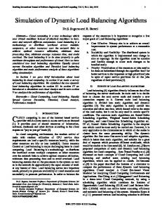
where Lmax is the maximum load on any process and L is the mean load over all processes. This metric measures the performance lost to imbalanced load or, conversely, the performance that could be reclaimed by balancing the load. Percent imbalance measures the severity of load imbalance. However, it ignores statistical properties of the load distribution that can provide insight into how quickly a particular algorithm can correct an imbalance. Statistical moments provide a detailed picture of load distribution that can indicate whether a distribution has a few highly loaded outliers or many slightly imbalanced processes. These properties impact which balancing algorithm will most efficiently correct the imbalance. Diffusive algorithms [7] can quickly correct small imbalances while the presence of an outlier in the load distribution may require more drastic, global corrections. Figure 1 shows the three most common statistical moments, standard deviation σ, skewness g1 and kurtosis g2 , where n is the number of processes and Li is the load on the ith process. Positive skewness means that relatively few processes have higher than average load, while negative skewness means that relatively few processes have lower than average load. A normal distribution of load implies skewness of 0. Higher kurtosis means that more of the variance arises from infrequent extreme deviations, while lower kurtosis corresponds to frequent modestly sized deviations. A normal distribution has kurtosis of 0. Statistical moments capture key information about load distri-
v u n u1 X σ=t (Li − L)2 n i=0 1 n
1 n
!3/2
(3)
(Li − L)2
i=0
1 n
n X (Li − L)4 i=0
g2 = 1 n
n X (Li − L)2
!2 − 3
22
Process 0 CompUnits = 7 CompWt = 16 MeasuredLoad = 11
1 1 2
3
2
2
2
1 7
2
1
3
Process 1 CompUnits = 4 CompWt = 8 MeasuredLoad = 5
4
2
Process 2 CompUnits = 5 CompWt = 16 MeasuredLoad = 10
Figure 2: Application Element-Aware Load Model (4)
i=0
Figure 1: Statistical Moments bution but are insufficient to evaluate the speed with which we can correct imbalance because they do not include information about the proximity of application elements in the simulation space. Table 1 uses several load distributions to show how the statistical moments fail to distinguish key properties. For simplicity, we show a one-dimensional interaction pattern of processes P0 ...P7 in which Pi and Pi+1 perform computation on neighboring domains. The figure shows that load metrics cannot distinguish cases (c) and (d) while the difficulty of correcting these load scenarios varies greatly if the computation is optimal when neighboring portions of the simulated space are assigned to the neighboring processes. In case (c), we could simply move the extra load on P1 to P0 , while in (d) the extra load from P7 must first displace work to P6 , P5 , and so on through P1 until the under-loaded P0 receives enough work.
4.
3 5
1
(Li − L)3
n X
2 2
n X i=0
g1 =
1 (2)
ELEMENT-AWARE LOAD MODEL
Parallel scientific applications decompose their physical domain into work units, which, in different applications, can be elements representing units of the simulated physical space, particles modeled, or random samples performed on the domain. Some application elements may involve more or less computation than others due to their physical properties or spatial proximity. Section 3 shows that a load model must be aware of the application elements and their interactions and placement in order to understand load imbalance and, more importantly, how to correct it. A model that does not include this information will fail to capture the effects of the proximity of elements in the simulation space and the mapping of the simulation space onto the process space. Our investigation of large-scale scientific applications has shaped our novel application-element-aware, application-independent load model that represents application elements and interactions between them. Our API enables the application to provide our framework with abstract application information at the granularity of application domain decomposition. This granularity allows our model to reflect application elements, their communication and dependencies, and their mapping to processes. Most load balancing algorithms analyze and redistribute work with the same granularity, which enables our framework to guide them. We provide a general methodology to map observed application performance accurately to the application elements at the appropriate granularity level. Figure 2 illustrates our load model: the edges represent bidirectional interactions between application elements. Solid edges
represent interactions within a process, while dashed edges represent interprocess communication. The relationships between application elements within the domain decomposition provide the communication structure and the relative weights of computation in the model. Node weights indicate the computation required for each element as anticipated by the application (i.e., the application load model). Importantly, we can correlate this information to wallclock measurements of the load on each process. The example in Figure 2 shows that Process 0 has 7 work units with an application anticipated load or relative computation weight of 16, and its work units have 4 channels of communication with elements on Process 1 with a total relative communication cost of 6. For example, we measure the load on Process 0 to be 11. We must carefully consider the difference in modeled and measured load. If the model is accurate, the two are linearly related. If they are not directly proportional, the application model is incomplete and could be improved. We discuss our methodology to evaluate abstract application information in Section 7.1. When we are satisfied with the model accuracy, we can use it to compute the load distribution metrics and to observe how the load is distributed throughout the process space in terms of application elements. Table 2 illustrates the versatility of our model by showing work unit mappings for three major types of scientific applications. Unstructured Mesh. In unstructured mesh applications, each cell in the mesh is an element. We represent the mesh connectivity with edges. In some unstructured mesh applications, the cells may require similar computation and we would anticipate unit computation per mesh cell. In others, the computation per cell may be proportional to the cell’s volume, and we reflect this in the weight of each node in our model. Table 2(a) shows an unstructured mesh application that performs a Monte Carlo algorithm on its mesh. In this case, the work is proportional to the number of samples in each mesh cell, so we use the sample count as the node weight. We show communication between neighboring grid cells as edges. Molecular Dynamics. In classical molecular dynamics applications and other N-body simulations, each individual body is an element. Edges reflect the simulated neighborhood of the bodies: each body is connected to others within a cutoff radius (i.e., those with which it interacts), as Table 2(b) shows. As we discuss in Section 7.1, we can select from several models for computation per element. Simple models assume that the work per body is constant, while others reflect the density of the body’s neighborhood. Empirical Model. Some applications, such as ParaDiS [6], use empirical models to anticipate computation per element. An application developer can construct this type of model by placing timers around important computation regions. Table 2(c) shows how ad hoc placement of timers may omit important load constituents.
Type of Application, elements and interactions
Sample Application Image
Representation in App.
Our Representation
(a) Unstructured Mesh 4
• e.g., particle transport or finite element applications • elements: cell volume or number of samples in each cell (Monte Carlo algorithms)
5
3
2
1
2
• interactions: mesh connectivity
(b) N-body
1
• e.g., Molecular Dynamics Applications
1
• elements: (sampled) molecules • interactions: molecules within range of interaction r (as defined by the application)
1 1
r
1 1
1 1
1 1
(c) Other - Empirical Model • e.g., ParaDiS (Section 6.3) • interactions: graph of process communication • elements: time in developer-defined ‘key’ routines (green); incomplete coverage of application behavmain ior (red) fn1
fn4
fn9
4.6s P1
fn3
P2
P3
2.1s
5.3s
4.1s
3.8s
5.1s P5
fn2 fn5
4.2s
P4 P0
P6
fn6 fn7
fn8
Table 2: Applications and Their Representation in Our Load Model
5.
LOAD BALANCE COST MODEL
In this section, we use our load model to evaluate the cost of two types of load balancing algorithm. Our cost model can guide selection of the best algorithm for specific imbalance scenarios.
5.1
Types of Load Balancing Algorithms
Global Algorithms. A global balancing algorithm [9, 19, 25] takes information about the load on all tasks and decides how to redistribute load evenly in a single step. Global decisions can be costly. Sequential implementations must process data for an entire parallel system. Parallel implementations can communicate excessively. Global algorithms also can require substantial element movement. However, if the cost of balancing is low, global algorithms balance load in a single step and correctly handle local minima and maxima. Diffusive Algorithms. A diffusive balancing algorithm [7] performs local corrections at each step and only moves elements within a local neighborhood in the logical simulation domain. Diffusive algorithms can take many steps to rectify a large imbalance because load can only move a limited distance. However, diffusive algorithms are scalable because they only require local information, and element movements can be mapped to perform well on high diameter mesh and torus networks used in the largest machines.
5.2
Cost Model for Balancing Algorithms
Our cost model captures the rebalancing characteristics of diffusive and global algorithms. Developers typically choose balancers based on their intuition about the scalability of particular algorithms. For example, one might expect the cost of a global balanc-
ing scheme to be higher than that of a diffusive algorithm at scale because the time required for an immediate rebalance outweighs the amortized cost of local diffusive balancing. The intuition is approximate and sometimes inaccurate. Our cost model provides a quantitative basis for selecting among algorithms. Table 3 summarizes the variables that we use to define this cost model. Our cost model only considers the current imbalance. Future imbalances are highly dependent on how the simulation evolves. Predicting them is generally infeasible (otherwise we could predict the result of the simulation). We assume a continuous evaluation of the imbalance in an application’s load leading to new balancing decisions when necessary. These decisions can consider the (observed) rate at which the application becomes imbalanced, and apply a global balancer when drastic changes are necessary or a diffusion scheme to handle more modest imbalances. A load balancing algorithm’s cost is the time to decide which elements to move plus the time required to move the elements: CBalAlg = CLbDecision + CDataMvmt
(5)
where BalAlg can be global or diffusion (i.e., Cglobal or Cdiffusion ). CLbDecision , the time to run the balancing algorithm, can be known a priori or derived using a performance model, such as a regression model over timings that vary the algorithm’s input parameters [15]. Typical parameters for the modeling approach include the input size (e.g., the number of vertices in the load model graph and the average number of edges per vertex) and the number of processes that a parallel balancing algorithm uses.
Variable
Definition
How Determined
Lave
Average process load
1 procs
procs X
Li
i=0
Li Di Lij γ convergence_steps Lmaxi ElementsMovedi CDataMvmt CLbDecision CBalAlgo AppTimeBalAlg steps
Load of process i Set of processes with elements that can be moved to process i Load of process j ∈ Di Load shifting coefficient in Algorithm 2 Number of steps for diffusive algorithm to converge Maximum process load at step i Largest number of elements moved to a process at step i Time required to send ElementsMovedi Runtime of load balancing algorithm, e.g., Cglobal and Cdiff Balancing algorithm cost: algorithm time plus redistribution time Total application runtime under BalAlg, e.g., AppTimediff Number of time steps that the application takes
Measured or estimated by Algorithm 2 Derived from edges in load model Measured or estimated by Algorithm 2 Provided by application, γ ≤ 1 Derived by simulating diffusion, Algorithm 2 Simulated (diffusion); ≈ Lave (global) Simulated (diffusion); ≈ Elementsmax L Lave (global) max −Lave Modeled empirically, α + βElementsMoved Measured or modeled empirically CLbDecision + CDataMvmt Modeled by cost model Arbitrary, same for global and diffusion algorithms
Table 3: Cost Model Variables Algorithm 2 Diffusion Simulation [7]
We define CDataMvmt as: CDataMvmt = α + βElementsMovedmax × elementsize
(6)
where the application provides elementsize, α is the start-up cost of communication (latency), and β is the per-element send time (bandwidth), determined empirically per platform. A more detailed model could capture network contention. For global balancing algorithms, we approximate the number of elements moved as: ElementsMovedglobal ≈ Elementsmax
Lave Lmax − Lave
(7)
where Elementsmax is the number of elements on the process with Lmax . We approximate the portion of the elements that we must move from the most loaded process as proportional to the load imbalance, which assumes that the load per element is approximately constant. Although this assumption is coarse (load balance would be trivial), we find this simplification works well in practice. The total cost of a load balancing algorithm is the application runtime when using the algorithm, which is the time to perform each computation step plus the cost of the algorithm at each step: steps
AppTimeBalAlg =
X
(CBalAlgi + Lmaxi )
(8)
i=0
where steps is the number of timesteps that the application takes, CBalAlgi is load balancing algorithm’s cost at step i, which is zero for a global algorithm in all steps other than the one in which load balancing is performed. The time for each step of the computation is the time taken by the most heavily loaded process, Lmax . For a global scheme, the total cost reduces to: AppTimeglobal = Cglobal1 + steps × Lave
(9)
since we assume that the global load balancing algorithm is only invoked in the first step. We estimate the time per computation step as Lave under the assumption that imbalance is corrected. For diffusion, we compute the total application time as: steps
AppTimediff =
X
(Cdiffi + Lmaxi )
(10)
i=0
To compute the total application time for diffusion, we have developed a diffusion simulator that mimics the behavior of diffusive load balancing algorithms. Algorithm 2 gives a high level overview of our diffusion simulator. We apply Algorithm 2 to our load model
Input. Li ← load of process i Di ← neighborhood of process i, defined in Load Model graph Lij ← load of process j ∈ Di γ ← coefficient for how much load can be moved in one timestep threshold ← lowest attainable level of imbalance for the application convergence_steps ← 0 1: All processes in parallel do 2: for timesteps do 3: if imbalance > threshold then 4: convergence_steps++ 5: end if X 6: Li = Li + γ(Li − Lij ) j∈Di
7:
ElementsMovedi = NumElementsi
X
γ(Li − Lij )
j ∈Di
8: NumElementsi = NumElementsi + ElementsMovedi 9: Lmaxi = max (Li ) ∀ processes at timestep i 10: ElementsMovedmaxi = max (ElsMovedi )∀ procs at step i 11: end for
to simulate the movement of load at each iteration. At each step, process i moves a portion of its load to its neighboring processes. We define a coefficient, γ, to model the amount of load that can be moved in one time step to reflect any application limitations (e.g., the maximum amount that domain boundaries can move in one time step). If the application does not limit element movement, γ = 1. Our algorithm accounts for local minima and maxima because it moves the simulated load through our graph based model similarly to data motion under an actual diffusive algorithm. Algorithm 2 records Lmaxi and ElementsMovedmaxi at each simulated step. We use those values in Equation 10. Additionally, Algorithm 2 defines an important metric, convergence steps, or the number of steps a diffusion algorithm takes to balance the load. This metric differentiates scenarios that a diffusion algorithm can correct quickly from those for which diffusion performs poorly. Algorithm 2 determines the costs required for Equation 10 much faster than the actual diffusion can be performed. We can evaluate its cost without perturbing the application. If the simulation predicts that diffusion will take too long, we can use a different load balancing algorithm such as a global load balancing scheme. We compare AppTimediff , AppTimeglobal , and AppTimenone to determine which load balance algorithm to use, where: AppTimenone = steps × Lmax1 We report the effectiveness of this decision in Section 7.2.
(11)
z
Algorithm 3 Benchmark Input. G ← graph of elements, where each process P is assigned a subgraph GP and remote edges represent interprocess communication 1: for P ∈ processes in parallel do 2: for timesteps do 3: for remote edges of GP do 4: Irecv/Isend messages 5: end for 6: for v ∈ G assigned to process P do 7: do_work(weightv ) 8: end for 9: MPI_Wait(all messages) 10: if directive to rebalance then 11: rebalance 12: end if 13: update info for load balancing framework 14: end for 15: end for
6.
BENCHMARKS AND APPLICATIONS
To evaluate our load and cost models, we conduct experiments with two large-scale scientific applications, ddcMD and ParaDiS, as well as a synthetic load balance benchmark that allows us to evaluate a larger variety of load scenarios and the performance of various load balancing algorithms for those scenarios.
6.1
Load Balance Benchmark
We use a benchmark to represent classes of load imbalance scenarios that occur in parallel scientific applications. Scientific applications can encounter varying initial load configurations, different patterns of element interactions, and different scenarios of how the imbalance evolves throughout the program. Our benchmark controls these variations to ensure a wide range of experiments. The main input to our benchmark is a directed graph with vertices that represent application elements and edges the communication/dependencies between them. We derive input graphs from a variety of meshes from actual simulations. We use a simple do_work(time) function that accesses an array in a random order. We tune this function for each architecture such that do_work(1) executes for one second. Algorithm 3 outlines our benchmark, which calls do_work for each graph vertex with the appropriate weights to represent the load scenario. We send an MPI message for each edge that connects vertices on different processes. Our experiments vary the size of the graph, vertex and edge weights, and the initial distribution. We can reassign each vertex to any process, as determined by the load balance framework.
6.2
ddcMD
ddcMD [8, 11] is a highly optimized molecular dynamics application that has twice won the Gordon Bell prize for high performance computing [11, 22]. It is written in C and uses the MPI library for interprocess communication. In the ddcMD model, each process owns a subset of the simulated particles and maintains lists of other particles with which its particles interact. To allocate particles to processes, ddcMD uses a Voronoi domain decomposition. Each process is assigned a point as its center; it “owns” the particles that are nearer to its center than any other. A Voronoi cell is the set of all points nearest to a particular center. Figure 3(a) shows a sample decomposition, with cells outlined in black and particles shown in red. Around each cell, ddcMD also maintains a bounding sphere that has a radius of the maximum distance of any atom in the domain to its center. During execution, atoms that a process owns can move outside of their cell. When this happens, ddcMD uses a built-in diffusion
ri ci
y
x
(a) ddcMD.
(b) ParaDiS.
Figure 3: Domain Decomposition in ddcMD and ParaDiS load balancer that uses a load particle density gradient calculation to reassign load. The balancer moves the Voronoi centers so that the walls of the Voronoi cells shift towards regions of greater density. Voronoi centers can only move a limited amount closer to neighboring cells. Voronoi constraints on the shape of cells also limit the possible distributions. To represent elements and the associated load, ddcMD uses three application-specific models: 1. Molecules: number of particles (molecules) per process; 2. Barriers: time each process spends outside of barriers; 3. Forces: time spent calculating interactions on each process. For our global load balancing algorithm, we use a point-centered domain decomposition method developed by Koradi [14]. Each step, we calculate a bias bi for each domain i. When the bias increases (decreases), the domain radius and volume increase (decrease). We assign each atom (with position vector x) to the domain that satisfies: |x − ci |2 − bi = minimal ,
(12)
where ci is the center of domain i, and we calculate the new centers as the center of gravity for the atoms in each cell. Although the Koradi algorithm is diffusive, we can run its steps independently of the application execution until it converges. Thus, our implementation is a global method since it only applies the final center positions in the application. We further optimize the algorithm by parallelizing it and executing it on a sample of the atoms rather than the complete set. Our experiments use a range of decompositions that exhibit different load balance properties by varying the placement of Voronoi cell centers. We evaluate all three models in Section 7.1, and vary load distributions in Section 7.2. We used two problem sets for ddcMD, a nanowire simulation and a condensation simulation. The nanowire simulation is a finite system of 133,280 iron (Fe) atoms that incurs imbalance due to uneven partitioning of the densely populated cylindrical body surrounded by vacuum. Atom interaction is modeled with EAM potentials. We ran the nanowire problem on 64 processes. The condensation simulation is a Lennard-Jones condensation problem with 2.5e+6 particles and the interactions modeled with Lennard-Jones potentials [13]. It incurs imbalance due to condensation droplets forming in some of the simulated domains. We ran the condensation simulation on 512 processes.
6.3
ParaDiS
ParaDiS [6] is a large-scale dislocation dynamics simulation used to study the fundamental mechanisms of plasticity. It is written primarily in C and uses MPI for interprocess communication. ParaDiS simulations grow in size as more time steps are executed. Thus, the application domain is spatially heterogeneous and the
distribution is recalculated periodically to rebalance the workload. ParaDiS uses a 3-dimensional recursive sectioning decomposition that first segments the domain in the X direction, then in the Y direction within X slabs, and finally in the Z direction within XY slabs. Figure 3(b) illustrates this decomposition method. ParaDiS uses an empirical model as an input to its load balancing algorithm. It estimates load using timing calipers around the computation that the developers consider most important for load balance. The load balancing algorithm adjusts work per process by shifting the boundaries of the sections. The size of neighboring domains constrains the magnitude of a shift and the algorithm does not move a boundary past the end of a neighboring section. This constraint makes the ParaDiS balancer a diffusion algorithm. For our experiments, we vary the distributions of the domain by varying the xyz decomposition of the domain such that x ∗ y ∗ z = nProcs. We use a highly dynamic crystal simulation input set for ParaDiS, with 1M degrees of freedom at the beginning of the simulation growing to 1.1M degrees of freedom by the end of the run. We ran this simulation on 128 processes.
Table 4: RMSE for Plots in Figure 4 Molecules
Barriers
Forces
15.917 0.444 0.138
25.769 0.079 0.008
16.095 0.057 0.007
imbalance kurtosis rank corr.
other processes. To calculate the rank correlation r of process loads between the application abstraction M and measured load L as, we first order all ranks based on the values of the developer-provided load abstraction and the measured load data. The resulting rank number for process i is stored in li and mi respectively, as is the mean rank in ¯ l and m. ¯ We then calculate the correlation with: n X (mi − m)(l ¯ i−¯ l) i=0 r= v uX n n X u t (mi − m) ¯ 2 (li − ¯ l)2 i=0
7.
EVALUATION
For all ParaDiS experiments, we use a Linux cluster that has 800 compute nodes, each with four quad-core 2.3 GHz AMD Opteron processors, connected by Infiniband. We use a similar cluster that has 1,072 compute nodes, each with four dual-core 2.4 GHz AMD Opteron processors connected by Infiniband for all ddcMD runs in Section 7.1. On both Linux systems, we use gcc 4.1.2 and MVAPICH v0.99 for the MPI implementation. We use a Blue Gene/P system with 1,024 compute nodes with 4 32-bit PPC450d (850MHz) cores each and 64 32-bit PPC450d I/O nodes for all ddcMD experiments in Section 7.2. On this system, we use gcc 4.1.2 for our measurement framework and compile ddcMD with xlC 9. To validate application models, we measure the work per process using Libra [10], a scalable load balance measurement framework for SPMD codes. Libra measures the time spent in specific regions of an application per time step using the effort model. In this model, time steps, or progress steps, model each step of the synchronous parallel computation, and fine-grained effort regions within these steps model different phases of computation. We extend Libra’s effort model to serve as input to our load model and add an interface to query load information during execution. We measure the computational load on each process by summing the time spent in all effort regions. Our load model couples these measurements with the application abstractions, allowing us to validate the abstractions against empirical measurements. We use PN MPI [20] to integrate Libra with our load model infrastructure. PN MPI stacks independent tools that use the MPI profiling interface [4], which we apply to combine Libra with our new load model component. PN MPI also supports direct communication among tools, which we use to exchange element interaction and performance information. Our tool stack imposes 3% overhead on average, an insignificant perturbation of application behavior.
7.1
Evaluating Application Abstractions
In this section, we evaluate the quality of ad hoc, developerprovided application load abstractions by comparing them with empirical measurements obtained from Libra. To quantify the quality of the abstractions, we report the accuracy with which they capture the measured load imbalance and the statistical moments of the measured load distribution, as defined in Section 3. For additional analysis, we validate application abstractions with a rank correlation metric. Rank correlation measures how accurately the abstraction ranks each process’s load relative to that of
(13)
i=0
To accommodate tied ranks correctly, we use Pearson’s correlation coefficient [17]. We now apply our abstraction evaluation methodology to ddcMD and ParaDiS. Figure 4(a) demonstrates how well the ddcMD abstractions capture the imbalance in the problem. Table 4 shows root mean squared error (RMSE) of load imbalance and the statistical moments calculated over our experiments. Abstractions based on the number of molecules and force computation overestimate the imbalance in the system, while the abstraction based on execution time excluding time spent at barriers underestimates the imbalance. Underestimating the imbalance leads to slower imbalance correction with a diffusion scheme because it is less aggressive than necessary. Alternately, overestimation pushes the limits of how much the load can be redistributed at each time step, and thus converges faster, as long as the overestimation correctly captures the relative loads. Figure 4(b) shows how the three ddcMD abstractions capture the kurtosis of the load distributions for each run; Table 4 shows the RMSE. The abstraction based on the number of molecules does most poorly, because much of the imbalance arise from imbalanced neighbor communication, which that abstraction omits. Figure 4(c) shows the rank correlation between the modeled and measured distributions for each of our test cases; Table 4 shows the corresponding RMSE. Again, abstractions based on time and force computation detect any outliers fairly well, while the abstraction based solely on the number of particles does worse. Overall, our analysis indicates that the force computation abstraction is the most accurate and, thus, the most suitable for use as input to the diffusion mechanism. To validate our conclusions, Figure 4(d) shows the number of steps to converge when the diffusion algorithm uses the three abstractions as input. We use a threshold of 12% imbalance because, as mentioned, ddcMD’s best achievable balance is limited by constraints on the shape of Voronoi cells in its domain decomposition. As predicted, the abstraction based on the force calculation is the most accurate and thus corrects the load most quickly. The abstraction based on the number of molecules outperforms the Barrier abstraction, partly because the former overestimates the imbalance making the diffusion scheme take more drastic measures and arrive at a balanced state sooner. Figure 5(a) shows the accuracy with which the ParaDiS application abstraction represents its load imbalance. Figure 5(b) shows the rank correlation of actual and modeled load distributions. The figures show that the abstraction is somewhat inaccurate, which we suspected because it does not include certain major phases of the
4
ddcMD
70 60 50 40 30
3 2 1 0
20 -1
10 0
10
20
30
40
50
60
70
80
-2 -1.5
90
-1
-0.5
Measured Load Imbalance (%)
ddcMD
1.5
2
2.5
3
30 25 20 15 10
3.5
10
15
0.85 0.8 0.75
30
35
40
ParaDiS Accurate Modeled
1.02 1
3.5e+11
Rank Correlation
0.9
25
(a) % imbalance in runs
Molecules Barriers Forces
4e+11
0.95
20
Measured Load Imbalance (%)
ddcMD
4.5e+11
Time till Convergence
Rank Correlation
1
35
(b) Kurtosis of load distributions
Accurate Molecules Barriers Forces
1
0.5
Accurate Modeled
Measured Kurtosis
(a) % imbalance in runs 1.05
0
ParaDiS
40
Accurate Molecules Barriers Forces
80
Modeled Kurtosis
Modeled Load Imbalance (%)
5
Accurate Molecules Barriers Forces
90
Modeled Load Imbalance (%)
ddcMD
100
3e+11 2.5e+11 2e+11 1.5e+11 1e+11
0.98 0.96 0.94 0.92 0.9
5e+10 0.88
0.7
0
10
20
30
40
50
60
Experiment
70
0
0
10
20
30
40
50
60
70
80
Experiment (sorted by Force model convergence time)
(c) Rank correlation of load distributions (d) Steps for diffusion algorithm to converge Figure 4: Evaluation of Three ddcMD Models computation that are captured by the measurements; the developers only measure the main force computation. Our load model in conjunction with Libra’s data shows that this fails to capture the behavior of communication, collision detection, and remesh phases. When we compare ParaDiS’s calipers to Libra’s measurements of only the force computation, the model is quite accurate. Depending on the problem, these omitted regions comprise up to 15% of the execution time. We have communicated our findings to the application developers, and are working with them to optimize how the application reports load to the load balancer.
7.2
Cost Model Case Study
In this section, we evaluate how well our model selects the most effective load balancer for particular imbalance scenarios, and we further evaluate the net performance improvement achieved using our model. We use the cost model defined in Section 5 to select the load balancing algorithm that would lead to the shortest runtime of our benchmark. We then apply our cost model to the global and diffusive load balancing schemes in ddcMD. For our benchmark, we compare total application runtime when using the following load balancing algorithms: 1. Global: Correcting imbalance during the first time step using Zoltan’s graph partitioner [9]; modeled by Equation 9; 2. Diffusive: Correcting imbalance at every time step using the Koradi method [14]; modeled by Equation 10; 3. None: No correction; modeled by Equation 11. We conduct runs spanning 2 to 64 processes with graphs with between 8,000 and 512,000 vertices and varying weights and initial decompositions. Figure 6(a) shows initial imbalance in the benchmark runs; we chose these initial imbalance scenarios because they are representative of some of the application runs we observed. Figure 6(b) shows that our load model correctly selects the algorithm that achieves the lowest runtime in 87% of the cases, tracing the curve with highest performance improvement for most of the
0
5
10
15
20
25
30
35
Experiment
(b) Rank correlation of load distributions Figure 5: ParaDiS Model Evaluation
experiments. In most cases, our model chooses the global algorithm. This algorithm performs very well in 96% of the cases, but 4% of the time, its high algorithmic and redistribution cost (as modeled by Equation 5) outweighs the performance benefit so it incurs a 35% performance penalty. In these cases, the diffusive algorithm outperforms the global algorithm, and our model correctly chooses it instead. In the only cases where our model does not choose the correct algorithm, it only suffers a penalty of 5.43% because these were scenarios where the global and diffusive algorithm performed within 6% of each other. On average, using our model can achieve a 49% performance gain while the next best alternative, the global algorithm, achieves 48% overall improvement in runtime. While the diffusive algorithm performed much worse than either of these overall (averaging net gains of only 3% over doing nothing), our model is still able to exploit it in the rare cases where it did outperform the global algorithm, leading to significant gains in these scenarios and more reliable performance across the board. For these cases, the diffusive algorithm performs significantly better than Zoltan, and using our model can prevent performance loss for workloads that contain many such pathological runs. For evaluating the performance of our model for ddcMD, we applied it to the input sets also used in Section 7.1; their initial load properties are demonstrated in Figures 4 (a-c). Our model selected among the following load balancing algorithms: 1. Global: Correcting imbalance during the first time step using the Koradi method [14] several times to mimic a method that corrects the imbalance in one step; modeled by Equation 9; 2. Diffusive: Correcting imbalance at every time step using the ad hoc Voronoi decomposition method with the Forces abstraction evaluated in Sec. 7.1 as input; modeled by Eqn. 10; 3. None: no correction; modeled by Equation 11. Table 5 shows runtimes of the load balancing algorithms for several imbalance scenarios in the nanowire simulation. These
% improvement over None
Measured Load Imbalance (%)
100 98 96 94 92 90 88 86 84
0
5
10
Benchmark
100
Imbalance
102
15
20
80
40 20 0 -20
0
5
10
15
20
25
Experiment (sorted by Load Model improvement)
Benchmark Input
None Global Diffusive Load Model
50
60
-40
25
ddcMD
None Global Diffusive Load Model
% improvement over None
Benchmark
104
(a) Starting Imbalance of Benchmark Runs (b) Model Performance on Benchmark Runs
0
-50
-100
-150
0
10
20
30
40
50
60
70
80
Experiment (sorted by Load Model improvement)
(c) Model Performance on ddcMD Runs
Figure 6: Evaluation of our Load Model on Benchmark and ddcMD
Load on each Process
Orig. Load
(a)
3 2 1 0
Diffus. Global Model
226
212
248
diff.
344
459
269
global
286
355
239
global
270
267
235
global
0 1 2 3 4 5 6 7 8 9 10 11 12 13 14 15
Load
(b)
3 2 1 0 0 1 2 3 4 5 6 7 8 9 10 11 12 13 14 15 3 2 1 0
Load
(c)
0 1 2 3 4 5 6 7 8 9 10 11 12 13 14 15 3 2 1 0
Load
(d)
0 1 2 3 4 5 6 7 8 9 10 11 12 13 14 15
Table 5: Sample ddcMD Imbalance Scenarios (seconds)
cases ran on 64 processors organized as a 4x16 process grid. Table 5 shows the relative load in the beginning of the simulation, with darker sections representing higher load and lighter blue representing lower load for the particular process. For each of these, we show the execution time without load balancing, the execution time with the diffusion algorithm, and the execution time using the global algorithm. We run the nanowire simulation for 200 time steps. The diffusion algorithm has a cost (as defined in Equation 5) of 0.01 seconds per simulation step. The global load balancing method incurs a one-time cost of 9 seconds. In all cases, our cost model guides the selection of the appropriate balancing algorithm. Figure 6(c) shows that our load model correctly selects the best algorithm in 96% of the cases, tracing the curve of the best performing algorithm. Because the Koradi algorithm improves the performance in 82% of the cases with an average performance gain of 14%, our model correctly selects it in most cases. The ad hoc Voronoi algorithm consistently performs worse and is only selected by the model in a few cases where its performance improvement outweighs the high cost of Koradi; overall, the model achieves a 19% gain over the ad hoc Voronoi algorithm. While our experiments are designed to explore a range of values, a suite of production runs might contain a variety of pathological cases, and our model will allow for a code to perform well even in the cases where the otherwise preferred balancing algorithm will perform poorly. Our model provides a means to select the appropriate load balancing algorithm at runtime without developer intervention, correctly selecting the algorithm that achieves the lowest runtime in up to 96% of the cases, achieving a 19% gain over selecting a single balancing algorithm for all cases.
8.
RELATED WORK
Previous work has focused on load measurement and finding sources of imbalance. Efficient, scalable measurement of load [12, 24] identifies whether load imbalance is a problem for a particular application. Imbalance attribution [23] provides insight into the source code locations that cause imbalance. Our load model takes advantage of existing tools [10] and their measurements, and combines them with knowledge of the application elements and their interactions. This combination improves understanding of computational load in terms of application elements. Many applications that suffer from load imbalance implement their own load balancing algorithms that are usually tightly coupled with application data structures and cannot be used outside of the application. Some rely heavily on geometric decomposition of the domain (i.e., hierarchical recursive bisection [6]). AMR applications can order boxes according to their spatial location by placing a Morton space filling curve [16] through the box centroids to increase the likelihood that neighboring patches reside on the same process after load balancing [27]. N-body simulations either explicitly assign bodies to processes or indirectly assign bodies by assigning subspaces to processes using orthogonal recursive bisection [2], oct-trees [21, 26], and fractiling [1]. These examples require application developers to construct an ad hoc model of per-task load. These abstractions are frequently inaccurate because they omit a significant subset of computational costs, or they fail to consider the platform. Our load model enables evaluation of the application abstractions, thus ensuring that the computation costs are correctly assigned prior to being used to correct the imbalance. Another common approach to load balancing uses suites of partitioners that work with mesh or graph representations of computation in the applications (e.g., ParMetis [19], Jostle [25], Zoltan [9]). Users of these partitioners must supply information about the current state of the application and the system, which again must be application specific. Thus, they may provide inaccurate or incomplete information. Further, partitioners do not have sufficient information to decide when to load balance, placing a further burden on the application developer. Our load model enables actionable evaluation of load imbalance, and can help a developer decide when to rebalance and whether the repartitioner is a good balancing algorithm for a particular type of imbalance. Charm++ [3, 5] provides a measurement-based load balancing framework that records the work represented by objects and objectto-object communication patterns. The load balancer can migrate the objects between process queues. While this approach may work well when the application developers can decompose their computation into independent objects, many applications cannot. In other cases, Charm++ can over-decompose the domain [18] and then bal-
ance load by moving virtual processors from overloaded physical processors to the underloaded ones. This approach can impose extra communication overhead for tightly coupled applications. In more recent work, Charm++ explores hierarchical approaches to load balancing [28]. Our model’s ability to evaluate the load in an actionable manner could thus provide a sound basis to choose the best level at which to balance the load.
[9]
[10]
9.
CONCLUSIONS
We have presented a novel load model based on application elements and their interactions. Our load model establishes a mapping between application elements and computation costs while maintaining information on dependencies between application elements. Our load model enables an application-independent representation of load distribution and can form the basis for a new generation of generic, yet element-aware load balance tools. We have shown that our element-aware approach overcomes deficiencies of conventional statistical load metrics, which fail to represent the element interaction information. Using our element-aware load model, we developed a new set of actionable metrics that accurately characterize load distribution. We have demonstrated the effectiveness and versatility of our load model on several case studies. We have provided a mechanism to evaluate and to contrast several application-provided abstractions. We have used our load model to analyze the load imbalance in two production applications. Finally, we evaluated the ability of available load balance schemes to correct imbalance. In all experiments, adding the application element interaction information to the load data was critical to understanding and analyzing the application’s load behavior.
10.
REFERENCES
[1] I. Banicescu and S. Flynn Hummel. Balancing processor loads and exploiting data locality in N-body simulations. In ACM/IEEE Conf. on Supercomputing, 1995. [2] M. J. Berger and S. H. Bokhari. A partitioning strategy for nonuniform problems on multiprocessors. IEEE Transactions on Computers, 1987. [3] A. Bhatelé, L. V. Kalé, and S. Kumar. Dynamic topology aware load balancing algorithms for MD applications. In ACM SIGARCH Intl. Conf. on Supercomputing, 2009. [4] S. Browne, J. Dongarra, N. Garner, G. Ho, and P. Mucci. A portable programming interface for performance evaluation on modern processors. Intl. Journal of High Performance Computing Applications, 14(3), 2000. [5] R. K. Brunner and L. V. Kalé. Handling application-induced load imbalance using parallel objects. Par. and Distr. Comp. for Symbolic and Irregular Applications, 2000. [6] V. Bulatov, W. Cai, J. Fier, M. Hiratani, G. Hommes, T. Pierce, M. Tang, M. Rhee, K. Yates, and T. Arsenlis. Scalable line dynamics in ParaDiS. In Supercomp., 2004. [7] G. Cybenko. Dynamic load balancing for distributed memory multiprocessors. Journal of Par. and Distr. Comp., 1989. [8] B. R. de Supinski, M. Schulz, V. V. Bulatov, W. Cabot, B. Chan, A. W. Cook, E. W. Draeger, J. N. Glosli, J. A. Greenough, K. Henderson, A. Kubota, S. Louis, B. J. Miller, M. V. Patel, T. E. Spelce, F. H. Streitz, P. L. Williams, R. K. Yates, A. Yoo, G. Almasi, G. Bhanot, A. Gara, J. A. Gunnels, M. Gupta, J. Moreira, J. Sexton, B. Walkup, C. Archer, F. Gygi, T. C. Germann, K. Kadau, P. S. Lomdahl, C. Rendleman, M. L. Welcome, W. McLendon, B. Hendrickson, F. Franchetti, S. Kral, J. Lorenz, C. W.
[11]
[12] [13]
[14]
[15]
[16] [17] [18]
[19]
[20] [21] [22]
[23]
[24]
[25] [26] [27]
[28]
Uberhuber, E. Chow, and U. Catalyurek. BlueGene/L applications: Parallelism on a massive scale. Intl. Journal of High Performance Computing Applications, 22(1), 2008. K. Devine, E. Boman, R. Heaphy, B. Hendrickson, J. Teresco, J. Faik, J. Flaherty, and L. Gervasio. New challanges in dynamic load balancing. Applied Numerical Mathematics, 52(2-3), 2005. T. Gamblin, B. R. de Supinski, M. Schulz, R. Fowler, and D. A. Reed. Scalable load-balance measurement for SPMD codes. In ACM/IEEE Conf. on Supercomputing, 2008. J. N. Glosli, K. J. Caspersen, J. A. Gunnels, D. F. Richards, R. E. Rudd, and F. H. Streitz. Extending stability beyond CPU millennium: A micron-scale atomistic simulation of Kelvin-Helmholtz instability. In Supercomputing, Nov. 2007. K. A. Huck and J. Labarta. Detailed load balance analysis of large scale parallel applications. In Par. Processing, 2010. J. E. Jones. On the determination of molecular fields. II. From the equation of state of a gas. Royal Society of London Proceedings Series A, 106:463–477, Oct. 1924. R. Koradi, M. Billeter, and P. GÃijntert. Point-centered domain decomposition for parallel molecular dynamics simulation. Computer Physics Communications, 2000. B. C. Lee, D. M. Brooks, B. R. de Supinski, M. Schulz, K. Singh, and S. A. McKee. Methods of inference and learning for performance modeling of parallel applications. In Principles and Practices of Parallel Programming, 2007. G. Morton. A computer oriented geodetic data base and a new technique in file sequencing. IBM tech report, 1966. J. L. Myers and A. D. Well. Research design and statistical analysis. Lawrence Erlbaum Associates Publishers, 2003. E. R. Rodrigues, P. O. A. Navaux, J. Panetta, A. Fazenda, C. L. Mendes, and L. V. Kale. A comparative analysis of load balancing algorithms applied to a weather forecast model. In Comp. Architecture and High Perf. Comp., 2010. K. Schloegel, G. Karypis, and V. Kumar. A unified algorithm for load-balancing adaptive scientific simulations. In ACM/IEEE Conf. on Supercomputing, 2000. M. Schulz and B. R. de Supinski. PN MPI tools: A whole lot greater than the sum of their parts. In Supercomputing, 2007. J. P. Singh, C. Holt, J. L. Hennessy, and A. Gupta. A parallel adaptive fast multipole method. In Supercomputing, 1993. F. Streitz, J. Glosli, M. Patel, B. Chan, R. Yates, B. de Supinski, J. Sexton, and J. Gunnels. 100+ TFlop solidification simulations on BlueGene/L. In Supercomputing, 2005. N. R. Tallent, L. Adhianto, and J. M. Mellor-Crummey. Scalable identification of load imbalance in parallel executions using call path profiles. In Supercomputing, 2010. N. R. Tallent, J. M. Mellor-Crummey, M. Franco, R. Landrum, and L. Adhianto. Scalable fine-grained call path tracing. In Intl. Conf. on Supercomputing, 2011. C. Walshaw and M. Cross. Parallel optimisation algorxithms for multilevel mesh partitioning. Parallel Computing, 2000. M. S. Warren and J. K. Salmon. A parallel hashed oct-tree N-body algorithm. In Conf. on Supercomputing, 1993. A. M. Wissink, D. Hysom, and R. D. Hornung. Enhancing scalability of parallel structured AMR calculations. In ACM SIGARCH Intl. Conf. on Supercomputing, 2003. G. Zheng, A. Bhatele, E. Meneses, and L. V. Kale. Periodic hierarchical load balancing for large supercomputers. Journal of High Perf. Comp. App., 2010.