Quantifying the time course of similarity Andrew T. Hendrickson (
[email protected]) Daniel J. Navarro (
[email protected]) School of Psychology, University of Adelaide
Chris Donkin (
[email protected]) School of Psychology, University of New South Wales Abstract Does the similarity between two items change over time? Previous studies (Goldstone & Medin, 1994; Gentner & Brem, 1999) have found suggestive results but have relied on interpreting complex interaction effects from “deadline” decision tasks in which the decision making process is not well understood (Luce, 1986). Using a self-paced simple decision task in which the similarity between two items can be isolated from strategic decision processes using computational modeling techniques (Ratcliff, 1978), we show strong evidence that the similarity between two items changes over time and shifts in systematic ways. The change in similarity from early to late processing in Experiment 1 is consistent with the theory of structural alignment (Gentner, 1983; Goldstone & Medin, 1994), and Experiment 2 demonstrates evidence for a stronger influence of thematic knowledge than taxonomic knowledge in early processing of word associations (Lin & Murphy, 2001). Keywords: similarity; temporal dynamics; hierarchical modeling; reaction time; drift-diffusion model;
Introduction Similarity plays an important role in cognitive science. Theories of categorization, induction and memory are all substantially reliant on some notion of stimulus similarity. Empirically, measures of stimulus similarity are used to supply mental representations via statistical techniques like multidimensional scaling, additive clustering and others. Yet similarity itself is notoriously slippery. It cannot be defined logically, on the basis of shared properties (Goodman, 1972), and it is sensitive to a variety of factors that suggest that the sense of similarity is not a primitive, but rather is constructed on the fly by the cognitive system (Medin, Goldstone, & Gentner, 1993). From this perspective, our theories must not merely describe the information people use to judge similarity: we must also consider when different sources of information become available to the decision maker. The answer to this question is not obvious: stimulus features might vary in their salience, in the amount of cognitive processing required to activate them, and in the ease by which they can be cued and recalled from memory. Any of these factors could influence when these features can contribute to judging similarity. To the extent that they do, the perceived similarity between two items should systematically change during the time course of the decision. Detecting these changes with empirical measures has proven difficult. Some studies (Goldstone & Medin, 1994; Gentner & Brem, 1999) have found suggestive results, relying on “deadline” tasks that force participants to respond after a fixed amount of time. In these designs, an interaction effect
between choice probabilities and response deadline is interpreted as the signature of time-dependent similarity, generally using ANOVA or related techniques. Yet, as the literature on choice response times indicates (Luce, 1986), there is no reason to expect that human choice probabilities will be welldescribed using the linear model underpinning ANOVA, nor is there any reason to believe that people do not adapt their decision criteria to suit a response deadline, opening up the possibility that these effects are merely artifacts of strategic behavior and do not reflect true differences in the underlying similarity perceived by participants. Our goal in this paper is to address these limitations using standard methods for modeling choice response times (Ratcliff, 1978). In doing so we replicate effects pertaining to structural alignment in similarity (Goldstone & Medin, 1994) and the taxonomic/thematic distinction (Gentner & Brem, 1999), and in both cases are able to demonstrate novel findings.
Choice response time in similarity based tasks The experimental framework we rely on is a standard two alternative forced choice task. Unlike “deadline” tasks that force participants to respond before an experimentercontrolled cutoff, we employ a subject-controlled design that allows participants to respond when they are ready. This design is the standard task in the literature on simple decisions (e.g. Luce, 1986). The response time is manipulated indirectly using an instructional manipulation: participants are asked either to respond as fast as possible or to respond as accurately as possible. The advantage to this manipulation is that its properties are well understood, and psychologists have developed computational models that can cleanly disentangle the accumulation of similarity evidence over time from the decision strategies of how and when to use that information. In essence, instead of relying on ANOVA to do the statistical inference, we rely on customized statistical models that are derived directly from standard psychological theory: in this case, we rely on a hierarchical extension of the drift-diffusion model (Ratcliff, 1978). The diffusion model treats a choice problem as a process of evidence accumulation that unfolds over time. The average rate of evidence accumulation is referred to as the drift rate: in a similarity-based decision, it acts as a measure of the relative similarity among the choice options. Evidence accrues until a sufficient amount of evidence is reached. The amount of evidence required is captured by a boundary sep-
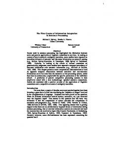
Figure 1: A sample trial from Experiment 1 composed of two panels. This trial shows a stimulus with 2 MIPs (yellow and brown squares in identical positions) and 2 MOPs (the green and blue squares are in different positions). Because the green and blue squares are not in the same position, these are DIFFERENT items.
aration parameter, and is assumed to be under the control of the participant. In these tasks drift rates capture the underlying similarity signal and the boundary separation parameter describes the decision strategy used to make choices about similarity.1
Experiment 1: Structural alignment processes An early investigation of how similarity unfolds over time comes from the work of Goldstone and Medin (1994), and focuses on structural alignment. Inspired by work on analogical reasoning, Goldstone and Medin (1994) proposed a formal theory of how people assess the similarity between structured stimuli. To give a simple example, consider the stimuli shown in Figure 1. Each “cross” stimulus consists of four “slots” each of which can be occupied by squares of different color. The spatial arrangement of the slots ensures that the stimuli are not merely four blobs of color: instead, they are organized into a specific configuration, ensuring that the two items shown in Figure 1 are distinct. Inspired by theories of analogical reasoning (Falkenhainer, Forbus, & Gentner, 1989; Gentner, 1983, 1989), Goldstone and Medin (1994) proposed a formal model of similarity (SIAM) that makes a clear prediction about how such stimuli are processed. The raw featural information (i.e., which blobs of color are present) is processed quickly and provides the first impressions of similarity, not dissimilar to how similarity is assessed in simple featural models (Tversky, 1977). The relational information that allows the colors of one stimulus to be matched against colors in another stimulus arrives more slowly, because the cognitive system is engaged in an active process of aligning the representations of one stimulus against the other (Falkenhainer et al., 1989; Gentner, 1983, 1989). Experiment 2 from Goldstone and Medin (1994) tested this idea using the “cross” stimuli shown in Figure 1. Participants were presented with pairs of stimuli and asked to judge if they were identical or not (i.e., a same-different task). To characterize a pair of stimuli, they introduced the following 1 The full diffusion model is somewhat more complex than this, but given that it is a standard model for choice tasks we omit all the details in the interests of brevity. In all our model fitting, the only parameters that were allowed to vary across conditions were drift and boundary separation, so we restrict the discussion only to these relevant aspects of the model.
Condition Stimulus A Stimulus B Count 0 MIPS 0 MOPS ABCD EFGH 50 0 MIPS 2 MOPS ABCD BAEF 50 2 MIPS 0 MOPS ABCD ABEF 50 0 MIPS 4 MOPS ABCD BCDA 50 ABCD ABDC 50 2 MIPS 2 MOPS SAME (4 MIPS) ABCD ABCD 250 Table 1: The six stimulus conditions in Experiment 1. The letters A through H indicate unique randomly chosen colors, and each column corresponds to one of the four positions in the cross. Condition names reflect the number of MIPs and MOPs in each condition, and the count column indicates the number of presentations of each condition.
terminology. If the same color appears in the same position for both stimuli, that feature is a match in place (MIP). If the same color appears in a different position it is a match out of place (MOP). A color that appears in one stimulus but not the other is a mismatch. The qualitative prediction made by Goldstone and Medin (1994) is that during the initial stage of processing there is no difference between MIPs and MOPs, because the featural information (color) is present but no relational mappings between the stimuli have been attempted. In essence: under time pressure, MOPs and MIPs should both count as evidence in favor of choosing “same”, but when more time is presented only MIPs should count as evidence for choosing “same” and MOPs should count as evidence for “different”.
Method Participants 262 workers on Amazon’s Mechanical Turk were recruited, 13 of whom were excluded for failing to complete the task. Of the remaining 249, 43% were female. Ages ranged from 18 to 66 years (mean: 34). 84% were from the USA, 14% from India, and 2% from other nations. Materials & Procedure The stimuli used in the task are illustrated in Figure 1. Each colored square was 40 pixels wide, and the positions of the crosses jittered slightly from trial to trial. Across all trials, there were 8 colors used (red, blue, green, yellow, turquoise, brown, gray, and orange). Colors were assigned randomly subject to the constraints outlined in Table 1, which lists 6 logically distinct stimulus conditions. On half of the 500 trials the two items were identical (i.e., 4 MIPS). On the other half of trials, there was at least one MOP or one mismatch. However, there were 5 distinct ways in which the items were different, as outlined in Table 1. In the 0 MIPS 0 MOPS condition, for instance, the items shared no color features, whereas in the 0 MIPS 4 MOPS the items share the same four colors, but no color appeared in the same position. In potentially the most confusing condition (2 MIPS 2 MOPS) the same four colors appear in both items, two in the same positions of both items and two with their positions swapped. The “cross” stimuli and the same-different task were explained to all participants. For the 116 participants assigned (randomly) to the speed condition, the instructions asked them to respond as quickly as possible. During the task itself, if they did not respond within 1000 ms they were in-
actions indicate that the odds of an effect exceed 1025 in all cases.2 However, the mere fact that the experimental manipulations were effective does not make clear precisely how the conditions influenced people’s perceptions of similarity and their decision strategy. To investigate this, we analyze the data in a more principled fashion using the diffusion model.
1500
Median RT
1000
500
Modeling at 4 M ch IP in s g) (M
2 2M M IP O s Ps
0 2M M IP O s Ps
4 0M M IP O s Ps
2 0M M IP O s Ps
0 0M M IP O s Ps
0
Stimulus Type Instructions
Accuracy
Speed
Figure 2: Median response times across stimulus types split into Speed and Accuracy instruction conditions. Response times in the Accuracy condition are influenced by the stimulus type but response times for the Speed condition are relatively constant. Error bars depict one standard error.
Accuracy (percent)
100
75
50
25
at 4 M ch IP in s g) (M
2 2M M IP O s Ps
0 2M M IP O s Ps
4 0M M IP O s Ps
2 0M M IP O s Ps
0 0M M IP O s Ps
0
Stimulus Type Instructions
Accuracy
Speed
Figure 3: Accuracy across stimulus types split into Speed and Accuracy instruction conditions. Participants in the Speed instruction condition incorrectly classify the 2 MIPS 2 MOPS stimuli in which all of the colors matched between the two panels but two colors were not in the same positions. Error bars depict one standard error.
formed that they were “too slow” after that trial. The remaining 133 participants were assigned to the accuracy condition and were encouraged to answer as accurately as possible, and were provided with “incorrect” feedback when their answer was wrong. Feedback was presented for 700 ms. Every 50 trials participants were given a break and told their accuracy and average response time in the previous block. During these breaks between blocks participants were reminded to be fast or accurate depending on their condition.
Results Figure 2 plots the median response time (RT) for each of the six stimulus types under both speed instructions and accuracy instructions. Figure 3 shows the corresponding plots for accuracy. Visual inspection of the plots suggests substantial and systematic differences in RT and accuracy across the stimulus types and instruction conditions. Bayesian mixed effects ANOVA (see Rouder, Morey, Speckman, & Province, 2012) confirms this: Bayes factors for all main effects and inter-
We use the diffusion model (Ratcliff, 1978) to jointly model the response time and accuracy at the individual subject level. To avoid overfitting the data we used a Bayesian hierarchical approach to estimate individual subject parameters (i.e. drift and boundary separation) as well as group-level distributions over these parameters (assumed to be normal).3 The boundary separation parameter was allowed to vary only as a function of the speed/accuracy instructions. A separate drift rate parameter was fit to each unique combination of stimulus condition and speed/accuracy instructions because previous work suggests that different information was likely to contribute early and late to similarity judgments for some stimulus conditions. The posterior distributions over drift and boundary separations are plotted in Figure 4. Not surprisingly, boundary separation is much smaller under speed instructions,4 indicating that people made their decisions faster and using less evidence. Similarly, the pattern of results for the drift parameter are very sensible with positive drift rates indicating evidence for “different” judgments. The most visually distinct stimuli (0 MIPS, 0 MOPS) have the highest drift rates, implying they are the most dissimilar. The identical stimuli (4 MIPS, 0 MOPS) have negative drift rates, indicating that people correctly detect them. The critical result arises when we compare drift rates for the same stimulus conditions under time pressure (speed condition) and without pressure (accuracy condition). The general pattern is similar, but there are two stimulus conditions that show noteworthy differences: whenever the items were different but only differentiated by the positions of the colors (i.e., 0 MIPS 4 MOPS and 2 MIPS 2 MOPS), the drift rate is much lower in the speed condition than the accuracy condition, even after accounting for the fact that drift rates decrease generally. This suggests that under time pressure people are differentially impaired at distinguishing between items that differ only in the configuration. In fact, in the most confusable case where only a single transposition differentiated the items 2 Model comparisons used a Bayesian analog of Type II tests in orthodox ANOVA to define relevant null and alternative hypotheses. 3 Model implementation used JAGS (Plummer et al., 2003; Wabersich & Vandekerckhove, 2014), ran three MCMC 1000sample chains with a 500-sample burn-in to approximate the posterior distribution over parameters. 4 For the sake of brevity we avoid quantifying the obvious fact that the results are significant. In every case when we refer to a difference, the posterior distributions in question are entirely nonoverlapping, implying that the data provide extremely strong evidence for a real difference.
Accuracy
Speed
we see a qualitative reversal: the drift rate for the 2 MIPS 2 MOPS condition is toward the incorrect response in the speed condition. This indicates that even after accounting for strategic effects people were substantially worse than chance when put under time pressure for that stimulus condition. Yet the drift rate for the same condition is toward the correct response in the accuracy condition, suggesting that later processing correctly interprets those items as different.
The exact fashion in which taxonomic and thematic knowledge shape similarity is somewhat unclear. Developmentally, there is evidence that thematic knowledge is acquired before taxonomic knowledge (Markman, 1991; Smiley & Brown, 1979). Although most studies assume taxonomic knowledge is central to categorization (Rosch, 1978), there is strong evidence that thematic knowledge can be just as powerful if not more so (Lin & Murphy, 2001), as well as studies suggesting that people are able to integrate both kinds of knowledge depending on task demands (Wisniewski & Love, 1998; Wisniewski & Bassok, 1999). Do both thematic and taxonomic knowledge follow the same time course? A “deadline” study by Gentner and Brem (1999) found modest evidence that when given a taxonomic judgment task thematic lures interfere with taxonomic processing. In experiment 2 we set out to determine the degree to which the Gentner and Brem (1999) results were due to a strategic shift in responding due to task constraints, a result of source confusion under time pressure, or an actual change from early to late processing in the similarity of taxonomic and thematic words. Furthermore, we test the degree to which the Gentner and Brem (1999) results are an asymmetric effect of thematic knowledge interfering with taxonomic processing or an overall interference between these two types of knowledge in early processing.
Discussion
Method
The pattern of results outlined above exactly matches the predictions made by Goldstone and Medin (1994) in a different task, and arguably provides stronger evidence than the original work. For the 2 MIPs 2 MOPs condition in particular we find a qualitative reversal: under time pressure people appear to process only the raw featural information, and because they do not detect the structural difference between the items they perform below chance. When more time is allowed participants are able to process the relational information in the stimuli and correctly detect the difference between the items. More generally, we see broad evidence that during the initial stages of processing stimulus similarity is heavily reliant on raw featural information, and only later do structural alignment processes shape perceived similarity.
Participants 416 workers were recruited through Amazon Mechanical Turk, 27 of whom were excluded for not completing the task or completing a substantially similar one. Of the 389 included participants, 43% were female. Ages ranged from 18 to 69 years old (mean: 35). 90% of participants 90% were from the USA, 9% from India, and 1% other.
2
●
3.0
● ●
● ● ●
1
●
2.5
● ●
0
●
−1
2.0
●
●
●
−2
●
Acc
Spd
00
02
04
20
22
same
00
02
04
20
22
same
Figure 4: Experiment 1 posterior distributions of hierarchical diffusion model parameters. The left panel shows the posterior distributions of the boundary separation parameters of the Speed and Accuracy instructions conditions. The right panel shows the posterior distributions of the drift rate parameters of the stimulus types across instruction conditions. The drift rate parameters are plotted such that positive drift rates are consistent with making DIFFERENT responses.
Experiment 2: Thematic and taxonomic knowledge We illustrate the generality of the diffusion modeling approach to disentangling the time course of similarity by applying it to a different kind of similarity judgment problem. In this experiment we look at a choice task in which people are shown a target word and asked to select which of two words is more closely related to the target. In particular, we consider decisions in which people must choose between thematic and taxonomic word associates. A taxonomic relation exists when two words pick out entities of the same kind (e.g., dog and wolf), whereas a thematic relation picks out entities that appear in similar situations (e.g., dog and bone).
Materials & Procedure Stimuli consisted of 93 triads composed of a target word, a taxonomically-related word and a thematically-related word. The triads were drawn from 6 previous studies (Gentner and Brem (1999), Lin and Murphy (2001), Ross and Murphy (1999),Smiley and Brown (1979), Wisniewski and Love (1998), Wisniewski and Bassok (1999)), presented in a random order, and can be found online.5 During the task the three items were displayed in a triangle with the target word at the top and the two response options positioned below to the left and right. Participants responded using the keyboard to select a response option. The task used two between-subjects manipulations, with participants assigned randomly. As before, participants were given speed instructions or accuracy instructions, with feedback given whenever the participant was slower than 1500ms (in the speed condition) or chose the wrong option (in the accuracy condition). The second manipulation instructed participants to focus on one kind of relation or the other. In the taxonomic condition they were asked to select the taxonomic associate, 5 https://gist.github.com/drewhendrickson/ e01dff14823b54ca54df
80
Thematic response (probability)
2000
60
Median RT
1500
40
1000
20
500
0
0 Taxonomic
Thematic
Taxonomic
Correct word associate Instructions
Accuracy
Speed
Instructions
Accuracy
Modeling Once again, we applied a hierarchical diffusion model in which boundary separation is influenced only by speed instructions, but allowed separate drift rates to be estimated for all four conditions. The posterior distributions over the relevant parameters are shown in Figure 7. On the left side the boundary separation is plotted. As one would expect, telling people to respond quickly caused the boundary separation to decrease: as before, people responded faster using less evidence. Of more interest is the fact that the effects on drift rates on the right side of Figure 7. This plot is drawn so that the correct answer always corresponds to positive drift rate. Under accuracy instructions, the drift rates are high and the posterior distribution for the taxonomic condition overlaps heavily with that of the thematic condition. When there is no time pressure, people find it equally easy to identify a thematic re-
Speed
1.0
2.2
●
2.0
0.6
0.8
●
●
1.6
●
0.2
0.4
●
Results The average accuracy in all four conditions is plotted in Figure 5, and the median RT is shown in Figure 6. For the accuracy data, Bayesian mixed effects ANOVA suggests that the data provide evidence of both a main effect of response instruction and an interaction term (Bayes factors for the relevant model comparisons are all > 1085 ), but evidence for a null effect of speed instruction (Bayes factor: 0.1). For the RT data, there is evidence only for a main effect of speed/accuracy (Bayes factor: 1020 ), but evidence for a null effect of response instruction (Bayes factor: 0.1). As before, however, a clearer picture emerges when we use the diffusion model to jointly model choice and response time.
Speed
2.4
●
1.8
whereas in the thematic condition they had to select the thematically related item. In both conditions, participants were shown an example of a target word (computer) and the task explained whether they were supposed to pick the taxonomic associate (calculator) or the thematic one (desk).
Accuracy
Figure 6: Median response times across Thematic and Taxonomic response instructions and split by Speed and Accuracy instruction conditions. Reaction time is strongly influenced by Speed instructions but shows no difference due to the response instructions. Error bars indicate one standard error. 1.2
Figure 5: Probability of selecting the thematic candidate word as a function of the four instructional conditions. There was a significant interaction between Speed and Accuracy instruction conditions and Thematic and Taxonomic response conditions. Error bars indicate one standard error.
Thematic
Correct word associate
Acc
Spd
Tax
Theme
Tax
Theme
Figure 7: Experiment 2 posterior distributions of hierarchical diffusion model parameters. The left panel shows the posterior distributions of the boundary separation parameters of the Accuracy and Speed instructions conditions. The right panel shows the posterior distributions of the drift rate parameters of the Taxonomic and Thematic instructions conditions in both the Accuracy and Speed instruction conditions. The drift rate parameters are plotted such that positive drift rates are consistent with the correct word choice.
lation as a taxonomic one. Under speed instructions, this symmetry breaks. It is not merely the case that the drift rates are lower, which would imply that people find it difficult to detect the differences between thematic-relatedness and taxonomic-relatedness under time pressure. In addition to this, the effect is asymmetric. The fact that drift rates are lower in the taxonomic condition than in the thematic condition implies that the thematic “signal” arrives faster than the taxonomic one.
Discussion As with Experiment 1, we find evidence that the time course of comparison is not homogeneous. When participants are given sufficient time to make choices, the information processing shows no bias towards thematic or taxonomic knowledge. However, under time pressure, people are better able to detect a thematic link than a taxonomic one. This result mirrors the developmental trajectory (Smiley & Brown, 1979), suggesting that not only is thematic knowledge acquired at a younger age, but that the processing of this information remains faster even in adulthood. Alternatively, it may be that
taxonomic information requires more deliberative processing and thus is slower and has less effect when people are pressured to respond quickly (Wisniewski & Bassok, 1999; Wisniewski & Love, 1998; Gentner & Brem, 1999).
General Discussion Employing the hierarchical drift-diffusion model to isolate the changes in similarity between early and late processing we find evidence in both experiments that the similarity between items changes in predictable ways over time. Both experiments show compelling evidence that the similarity between two items is not a static, stable value but one that emerges, shifts, and qualitatively changes signal over the first few seconds of processing. Critically, this difference between early and late similarity signals is not uniform across all conditions, in both experiments we find that the change in similarity influences some conditions and stimuli more than others. Interestingly, these conclusions are not straightforward or clear from statistical tests of the accuracy and reaction time data themselves. The strongest conclusions in both experiments emerge from the interpretation of the posterior distributions of the diffusion model evidence accumulation parameters after the effect of shifting decision strategies due to instructional manipulations are accounted for by the boundary separation parameters. These results appear to complement recent work showing that drift rates show systematic differences across speed and accuracy instructions in lexical decision tasks (Rae, Heathcote, Donkin, Averell, & Brown, 2014). In the current work we not only find that drift rates for accuracy conditions are larger than those for speed conditions, but we find that the difference between these two depends on the type of information in the choice task. Furthermore, these results suggest that changes over time to the set of included features, due to complexity, difficulty, or speed of processing, may be an additional explanation for the difference between early and late evidence accumulation.
Acknowledgments DJN received salary supported from ARC grant FT110100431. Research costs and salary support for ATH were funded through ARC grant DP110104949.
References Falkenhainer, B., Forbus, K. D., & Gentner, D. (1989). The structure-mapping engine: Algorithm and examples. Artificial Intelligence, 41(1), 1–63. Gentner, D. (1983). Structure-mapping: A theoretical framework for analogy. Cognitive Science, 7(2), 155–170. Gentner, D. (1989). The mechanisms of analogical learning. Similarity and Analogical Reasoning, 199, 199–241. Gentner, D., & Brem, S. K. (1999). Is snow really like a shovel? distinguishing similarity from thematic relatedness. In Proceedings of the twenty-first annual meeting of the Cognitive Science Society (pp. 179–184).
Goldstone, R. L., & Medin, D. L. (1994). Time course of comparison. Journal of Experimental Psychology: Learning, Memory, and Cognition, 20(1), 29–50. Goodman, N. (1972). Seven strictures on similarity. In Problems and projects. Bobs-Merril. Lin, E. L., & Murphy, G. L. (2001). Thematic relations in adults’ concepts. Journal of Experimental Psychology: General, 130(1), 3–26. Luce, R. D. (1986). Response times. Oxford University Press. Markman, E. M. (1991). Categorization and naming in children: Problems of induction. MIT Press. Medin, D. L., Goldstone, R. L., & Gentner, D. (1993). Respects for similarity. Psychological Review, 100(2), 254– 278. Plummer, M., et al. (2003). JAGS: A program for analysis of bayesian graphical models using gibbs sampling. In Proceedings of the 3rd international workshop on distributed statistical computing (DSC 2003). March (pp. 20–22). Rae, B., Heathcote, A., Donkin, C., Averell, L., & Brown, S. (2014). The hare and the tortoise: Emphasizing speed can change the evidence used to make decisions. Journal of Experimental Psychology: Learning, Memory, and Cognition, 40(5), 1226–1243. Ratcliff, R. (1978). A theory of memory retrieval. Psychological Review, 85(2), 59–108. Rosch, E. H. (1978). Principles of categorization. In E. H. Rosch & B. B. Lloyd (Eds.), Cognition and categorization. Hillsdale, NJ: Erlbaum. Ross, B. H., & Murphy, G. L. (1999). Food for thought: Cross-classification and category organization in a complex real-world domain. Cognitive Psychology, 38(4), 495– 553. Rouder, J. N., Morey, R. D., Speckman, P. L., & Province, J. M. (2012). Default bayes factors for anova designs. Journal of Mathematical Psychology, 56(5), 356–374. Smiley, S. S., & Brown, A. L. (1979). Conceptual preference for thematic or taxonomic relations: A nonmonotonic age trend from preschool to old age. Journal of Experimental Child Psychology, 28(2), 249–257. Tversky, A. (1977). Features of similarity. Psychological Review, 84(4), 327–352. Wabersich, D., & Vandekerckhove, J. (2014). Extending jags: A tutorial on adding custom distributions to jags (with a diffusion model example). Behavior Research Methods, 46(1), 15–28. Wisniewski, E. J., & Bassok, M. (1999). What makes a man similar to a tie? Stimulus compatibility with comparison and integration. Cognitive Psychology, 39(3), 208–238. Wisniewski, E. J., & Love, B. C. (1998). Relations versus properties in conceptual combination. Journal of Memory and Language, 38(2), 177–202.