QUANTILE BASED ESTIMATION OF SCALE AND ...

Q U A N T I L E B A S E D E S T I M AT I O N O F S C A L E A N D DEPENDENCE garth tarr

A thesis submitted in fulfilment of the requirements for the degree of Doctor of Philosophy

School of Mathematics and Statistics Faculty of Science University of Sydney 19 May 2014

Garth Tarr: Quantile based estimation of scale and dependence, Doctor of Philosophy, c 19 May 2014

Far better an approximate answer to the right question, which is often vague, than the exact answer to the wrong question, which can always be made precise. — John Wilder Tukey (1962)

ABSTRACT

The sample quantile has a long history in statistics. The aim of this thesis is to explore some further applications of quantiles as simple, convenient and robust alternatives to classical procedures. The first application we consider is estimating confidence intervals for quantile regression coefficients, however, the core of this thesis is the development of a new, quantile based, robust scale estimator and its extension to autocovariance estimation in the time series setting and precision matrix estimation in the multivariate setting. Chapter 1 addresses the need for reliable confidence intervals for quantile regression coefficients particularly in small samples. The existing methods for constructing confidence intervals tend to be based on complex asymptotic arguments and little is known about their finite sample performance. We consider taking xy-pair bootstrap samples and calculating the corresponding quantile regression coefficient estimates for each sample. Instead of estimating a covariance matrix based on these bootstrap samples, our approach is to take the appropriate upper and lower quantiles of the bootstrap sample estimates as the bounds of the confidence interval. The resulting confidence interval estimate is not necessarily symmetric; only covers admissible parameter values; and is shown to have good coverage properties. This work demonstrates the competitive performance of our quantile based approach in a broad range of model designs with a focus on small and moderate sample sizes. These results were published in Tarr (2012). A reliable estimate of the scale of the residuals from a regression model is often of interest, whether it be parametrically estimating confidence intervals, determining a goodness of fit measure, performing model selection, or identifying unusual observations. The robustness of quantile regression parameter estimates to y-outliers does not extend to the error distribution – extreme observations in the y space yield outlying residuals which can interfere with subsequent analyses. This led us to consider the more fundamental issue of robust estimation of scale. Chapter 2 forms the core of this thesis with its investigation into robust estimation of scale. Common robust estimators of scale such as the interquartile range (IQR) and the median absolute deviation from the median (MAD) are inefficient when the observations come from a Gaussian distribution.

iv

Rousseeuw and Croux (1993) propose a more efficient robust scale estimator, Qn , which is now widely used. We present an even more efficient robust scale estimator, Pn , which is proportional to the IQR of the pairwise means. The estimator Pn is the scale analogue of the Hodges-Lehmann estimator of location, the median of the pairwise means. When the underlying distribution is Gaussian, the Hodges-Lehmann estimator is considerably more efficient than the median however it is not as robust – similarly, Pn trades some robustness for significantly higher Gaussian efficiency. In the theoretical treatment, Pn is considered as a special case of a more general class of estimators – based on the difference of two quantiles of the pairwise means. For this class of estimators, assuming the observations are independent and identically distributed, we show that the influence function is bounded and establish asymptotic normality. Further extensions to Pn incorporate adaptive trimming to achieve the maximal breakdown value of 50%. The resulting adaptively trimmed scale estimator has enhanced performance at extremely heavy tailed distributions and is shown to be triefficient across Tukey’s three corner distributions amongst the set of estimators considered. The adaptively trimmed Pn also yields good results in the multivariate setting discussed in Chapter 4 The primary advantage of Pn over competing estimators is its high efficiency at the Gaussian distribution whilst maintaining desirable robustness and efficiency properties at moderately heavy tailed and contaminated distributions. The desirable efficiency properties of Pn are shown to be even more marked over competing scale estimators in finite samples. The results of this chapter have been published in Tarr, Müller and Weber (2012) and presented at ICORS 2011. Chapter 3 extends our robust scale estimator to the bivariate setting in a natural way as proposed by Gnanadesikan and Kettenring (1972). In doing so we move from estimating scale to estimating dependence. We show that the resulting covariance estimator inherits the robustness and efficiency properties of the underlying scale estimator. Motivated by the potential to extend the efficiency and robustness properties of Pn to the time series setting, Chapter 3 also considers the problem of estimating scale and autocovariance in dependent processes. We establish the asymptotic normality of Pn under short and mildly long range dependent Gaussian processes. In the case of extreme long range dependence, we prove a non-Gaussian limit result for the IQR, consistent with results found previously for the sample standard deviation and Qn . In contrast with the

v

results of Lévy-Leduc et al. (2011c) for a single U-quantile, namely Qn , the proof for the IQR, a difference of two quantiles, relies on the higher order terms in the Bahadur representation of Wu (2005). Simulation suggests that an equivalent result holds for Pn ; we state the conjectured result which will require the analogous Bahadur representation for U-quantiles under long range dependence. It is reasonably straightforward to extend the asymptotic results for the robust scale estimator to the corresponding robust autocovariance estimators. Various results from this chapter have been presented at ASC 2012 and EMS 2013. Classical robust estimators assume that contamination occurs within a subset of the observations, however in recent years there has been interest in developing robust estimators that perform well under scattered contamination. Chapter 4 looks at the problem of estimating covariance and precision matrices under cellwise contamination. A pairwise approach is shown to perform well under much higher levels of contamination than standard robust techniques would allow. Rather than using the Orthogonalised Gnanadesikan and Kettenring procedure (Maronna and Zamar, 2002), we consider a method that transforms a symmetric matrix of pairwise covariances to the “nearest” covariance matrix (in a Frobenius norm sense). We combine this method with various regularisation routines purpose built for precision matrix estimation. This approach works well with high levels of scattered contamination and has the advantage of being able to impose sparsity on the resulting precision matrix. Some preliminary results from this chapter have been presented at ICORS 2013.

vi

P U B L I C AT I O N S A N D P R E S E N TAT I O N S

Some of the ideas and figures from the first two chapters of this thesis have appeared in the following publications: Tarr, G., Müller, S., and Weber, N. C. (2012). A robust scale estimator based on pairwise means. Journal of Nonparametric Statistics, 24(1), 187–199. Tarr, G. (2012). Small sample performance of quantile regression confidence intervals. Journal of Statistical Computation and Simulation, 82(1), 81–94. A number of the results have been presented at the following conferences: Robust scale and autocovariance estimation. European Meeting of Statisticians, 2013, Budapest, Hungary. Robust covariance estimation via quantiles of pairwise means and applications. International Conference on Robust Statistics, 2013, St Petersburg, Russia. Robust scale estimation with extensions. Young Statisticians Conference, 2013, Melbourne, Australia. Robust covariance estimation with Pn . Australian Statistical Conference, 2012, Adelaide, Australia. Efficient and robust scale estimation. International Conference on Robust Statistics, 2011, Valladolid, Spain. Seminar presentations have been given at the following universities: Robust estimation of scale and covariance with Pn and its application to principal components analysis. University of NSW, School of Mathematics and Statistics, 2013, Sydney, Australia. Robust estimation of scale and covariance with Pn and its application to precision matrix estimation. University of Sydney, School of Mathematics and Statistics, 2013, Sydney, Australia.

vii

ACKNOWLEDGMENTS

I have been fortunate to have the unfailing support of a number of very talented and generous people over my time at the University of Sydney and the last four years in particular. Firstly, to Neville Weber and Samuel Müller, I could not have asked for more dedicated, patient and knowledgable supervisors. Their complementary skills have led to an interesting and varied thesis. Neville’s breadth of statistical and probabilistic understanding and his expertise in asymptotic arguments gave me the impetus and courage to continue to push outside my comfort zone. Samuel’s initial idea for the new scale estimator gave rise to the core of the thesis and his background in robustness provided inspiration for new directions. Their fanatical/rigorous/enthusiastic/fervent/dogged/rabid attention to detail lead to significant improvements in clarity and structure. They helped make me a better statistician and a better communicator. Though after suffering through many years of grammatical abuse, I fear I may have worn down Neville’s resolve against the split infinitive. I have been extremely lucky to have had many travel opportunities to network and peddle my statistical wares. I am grateful for the financial support I received from the University of Sydney’s Postgraduate Research Support Scheme, the School of Mathematics and Statistics’ statistics research group, the Statistical Society of Australia through their Golden Jubilee Travel Grant and my supervisors. I also want to thank my fellow PhD candidates, colleagues and students at the University of Sydney for making it an enjoyable few years. Ellis Patrick and Emi Tanaka who shared the journey with me from the beginning; many coffees with Justin Wishart, Patrick Noble, Luke Cameron-Clarke and Kellie Morrison; discussions at Hermanns with Michael Stewart, John Ormerod, Lisa Cameron and more recently Sanjaya Dissanayake, Tom Porter and Shila Ghazanfar. My eternal gratitude goes to my partner Georgie Philpott and my parents for their support and for defending me when my grandmother invariably asks why I am still at university.

viii

CONTENTS 1

quantile regression confidence intervals 1 1.1 Introduction 1 1.2 Overview of confidence interval construction techniques 1.2.1 Direct estimation 4 1.2.2 Rank inversion 4 1.2.3 Resampling methods 5 1.3 Simulation study 7 1.3.1 Heavy tailed errors 8 1.3.2 Skewed covariates 11 1.3.3 Multiple regression and heteroskedasticity 12 1.4 Conclusion 17

2

scale estimation 19 2.1 Introduction 19 2.2 Background theory 21 2.2.1 U- and U-quantile statistics 21 2.2.2 Generalised L-statistics 23 2.3 Review of robust scale estimation theory 24 2.3.1 Measures of robustness 24 2.3.2 Existing scale estimators 26 2.4 A scale estimator based on pairwise means 32 2.4.1 The estimator Pn 32 2.4.2 Properties of Pn 37 2.5 Relative efficiencies in finite samples 42 2.5.1 Design 43 2.5.2 Results 44 2.6 Conclusion 49

3

covariance and autocovariance estimation 3.1 Introduction 51 3.2 Robust covariance estimation 52 3.2.1 Properties 53 3.2.2 Simulations 56 3.3 Robust autocovariance estimation 61 3.4 Short range dependent Gaussian processes 64 3.4.1 Results for Pn 64

ix

51

3

contents

3.5

3.6 3.7 4

3.4.2 Results for gˆ P (h) 68 Long range dependent Gaussian processes 70 3.5.1 Parameterisation 73 3.5.2 Hoeffding versus Hermite decomposition 3.5.3 Interquartile range 76 3.5.4 Results for Pn 80 3.5.5 Results for gˆ P (h) 88 Simulations 92 Conclusion 97

covariance and precision matrix estimation 4.1 Introduction 100 4.2 Scattered contamination 102 4.3 Performance indices 105 4.3.1 Matrix norms 105 4.3.2 Other indices 107 4.3.3 Behaviour of performance indices 110 4.4 Pairwise covariance matrix estimation 116 4.4.1 OGK procedure 116 4.4.2 NPD procedure 118 4.4.3 Comparing OGK and NPD 119 4.5 Precision matrix estimation 121 4.5.1 GLASSO 122 4.5.2 QUIC 122 4.5.3 CLIME 124 4.6 Simulation study 125 4.6.1 Design 125 4.6.2 Results 127 4.7 Conclusion 137

Appendices

100

138

a quantile regression confidence intervals b

74

scale estimation 145 b.1 Finite sample correction factors 145 b.2 Implosion breakdown 147 b.3 Pairwise mean scale estimator code for R b.4 EM algorithm implementation 149

139

148

c covariance and autocovariance estimation c.1 Technical results 151

151

x

contents

c.2

c.3

c.4

c.5

c.1.1 Hadamard differentiability 151 c.1.2 Influence functions 151 Hermite ranks 152 c.2.1 Influence function of Pn 152 c.2.2 Empirical distribution function 154 c.2.3 Pairwise mean distribution function 155 Results for SRD processes 158 c.3.1 Convergence of empirical distribution functions c.3.2 Central limit theorem 159 c.3.3 Existing results for estimators 159 Results for LRD processes 161 c.4.1 Limit results for U-processes 161 c.4.2 Existing results for estimators 164 Relative efficiencies 167

d covariance and precision matrix estimation d.1 Generating precision matrices 168 d.2 Entropy loss results 169 d.3 PRIAL results 172 d.4 Log determinant results 173 bibliography

174

168

158

xi

LIST OF FIGURES

Figure 1.1 Figure 1.2 Figure 1.3 Figure 1.4 Figure 1.5 Figure 1.6 Figure 2.1 Figure 2.2 Figure 2.3 Figure 2.4 Figure 2.5 Figure 2.6 Figure 2.7 Figure 3.1 Figure 3.2 Figure 3.3 Figure 3.4 Figure 3.5 Figure 3.6 Figure 3.7 Figure 3.8 Figure 3.9 Figure 3.10 Figure 3.11 Figure 4.1 Figure 4.2 Figure 4.3 Figure 4.4 Figure 4.5

The check function, rt (u) 4 Coverage probabilities for the heavy tailed error model 9 Average confidence interval lengths for the heavy tailed error model 10 Coverage probabilities for the skewed covariate model 13 Average confidence interval lengths for the skewed covariate model 14 Coverage probabilities for the multiple regression model with heteroskedasticity 16 Finite sample MAD estimates 31 Breakdown value and efficiency of Pn (t ) 33 Finite sample relative efficiency of Pn (t ) 35 Influence functions at the Gaussian 39 Asymptotic relative efficiencies 40 Relative efficiencies at t distributions 45 Relative efficiencies at Tukey’s three corners 46 Asymptotic variance of covariance estimators 55 Relative efficiency of robust correlation estimators over various t distributions 58 Relative MSEs of robust correlation estimators over various t distributions 58 Efficiency of robust correlation estimators against r 60 MSEs of robust correlation estimators against r 60 Corruption and autocovariance estimators 62 Annual Nile river minima 71 ACF of the annual Nile river minima 72 Example LRD data series 93 Empirical densities for scale estimates 96 Empirical densities for autocovariance estimates 98 Scattered contamination 103 Eigenvalue distortion 109 Covariance matrix performance indices 111 Precision matrix performance indices 111 Increasing variance and precision matrix elements 112

xii

List of Figures

Figure 4.6 Figure 4.7 Figure 4.8 Figure 4.9 Figure 4.10 Figure 4.11 Figure 4.12 Figure 4.13 Figure 4.14 Figure 4.15 Figure 4.16 Figure A.1 Figure A.2 Figure A.3 Figure D.1 Figure D.2 Figure D.3 Figure D.4 Figure D.5

Increasing variance and the eigenvalues of precision matrices 114 Scattered contamination and covariance matrices 115 Scattered contamination and precision matrices 115 PRIAL results for estimated covariance matrices under moderate and extreme contamination 120 Precision matrix head maps 126 Example of the contaminating distribution 127 PRIAL results for CLIME with banded structures 130 PRIAL results for banded structures and p = 60 132 PRIAL results for banded, scattered and dense precision matrix structures with the QUIC procedure 133 Log determinant results for the GLASSO procedure 135 Entropy loss and Frobenius norm results for covariance matrices after using CLIME 136 Empirical coverage probabilities for the heavy tailed error model with n = 100 140 Empirical coverage probabilities for the heavy tailed error model with n = 150 141 Empirical coverage probabilities for the heavy tailed error model with n = 200 142 Entropy loss results for CLIME with extreme outliers 169 Entropy loss results with extreme outliers 170 Entropy loss results for QUIC with extreme outliers 171 PRIAL results for moderate outliers 172 Log determinant results 173

xiii

L I S T O F TA B L E S

Table 2.1 Table 2.2 Table 3.1 Table 3.2 Table 3.3 Table 4.1 Table A.1 Table A.2 Table A.3 Table A.4 Table B.1 Table B.2 Table C.1 Table C.2

Relative efficiencies at Tukey’s three corners 47 Triefficiencies of various scale estimators 48 MSEs under SRD processes 94 Average estimates from an ARFIMA(0, 0.1, 0) process Average estimates from an ARFIMA(0, 0.4, 0) process PRIAL results when there is no contamination 128 Summary output for Cauchy distributed errors 143 Summary output for t3 distributed errors 143 Summary output for t5 distributed errors 144 Summary output for standard Gaussian errors 144 Finite sample correction factors 145 Sampling distribution of pairs 147 Efficiencies for ARFIMA(0, 0.1, 0) processes 167 Efficiencies for ARFIMA(0, 0.4, 0) processes 167

xiv

95 97

ACRONYMS

ACF

autocorrelation function

CLIME

constrained L1 minimisation for inverse covariance matrix estimation

CDF

cumulative distribution function

CLT

central limit theorem

GLASSO

graphical lasso

IQR

interquartile range

LRD

long range dependent

MAD

median absolute deviation from the median

MCD

minimum covariance determinant

MSE

mean square error

MLE

maximum likelihood estimate

NPD

nearest positive definite

OGK

Orthogonalised Gnanadesikan Kettenring

OGKw

reweighted Orthogonalised Gnanadesikan Kettenring

PD

positive definite

PRIAL

percentage relative improvement in average loss

PSD

positive semidefinite

QUIC

quadratic inverse covariance

SD

sample standard deviation

SRD

short range dependent

xv

N O M E N C L AT U R E

a small number

e

IF( x; T, F ) influence function

bxc

the integer part of x

A

matrix transpose of A

|

I

indicator function

S

classical sample covariance matrix

S

covariance matrix

Q

precision matrix

F

standard Gaussian cumulative distribution function

f

standard Gaussian probability density function

D

!

converges in distribution

!

converges in probability

p

#

proportion of contamination

#⇤

breakdown value

F

cumulative distribution function

f

probability density function

Fn

empirical distribution function

G

cumulative distribution function of the kernels of a U-statistic

Gn

empirical distribution function of the kernels of a U-statistic

Hk

kth Hermite polynomial

ui

random error term

xvi

Q U A N T I L E R E G R E S S I O N C O N F I D E N C E I N T E R VA L S

1.1

introduction

Quantile regression, first introduced by Koenker and Bassett (1978), provides an alternative to least squares with numerous advantages, not the least being the ability to estimate the full conditional quantile function. However, a major drawback to the use of quantile regression is the lack of agreement on a single unified method for conducting inference on the parameters. The purpose of this chapter is to highlight the xy-pair bootstrap as a widely applicable method that has comparable performance to other more complicated confidence interval construction techniques. Numerous methods have been proposed, beginning with the direct estimation for standard errors of the parameters in the original Koenker and Bassett (1978) paper which was subsequently extended to the independent but not identically distributed case by Hendricks and Koenker (1992). In 1992, Gutenbrunner and Jureˇcková related the quantile regression parameters with the linear program used to calculate them, showing that the dual to the linear program allowed the application of rank inversion methodology to calculate confidence intervals directly. This was generalised by Koenker and Machado (1999) to allow for non-identically distributed errors. Naturally, resampling methods have also been applied to the quantile regression inference problem. One approach would be the residual bootstrap, however Efron and Tibshirani (1993) showed it to be severely lacking when the model does not satisfy the independent and identically distributed assumption. Using the nonparametric xy-pair bootstrap to estimate an asymptotic covariance matrix for the estimated parameters is an option. Another possibility is to use the percentile bootstrap which was shown to have asymptotically correct empirical coverage probabilities by Hahn (1995). However, the percentile bootstrap method has received little attention since then. Other, more abstract, resampling methods have been proposed. Parzen, Wei and Ying (1994) suggested exploiting the asymptotically pivotal subgradient condition. Another example is the Markov chain marginal boot-

1

1

1.1 introduction

strap by He and Hu (2002), applied to quantile regression estimates in Kocherginsky, He and Mu (2005) and extended to the non-identically distributed case in Kocherginsky and He (2007). Further, a version of the generalised or weighted bootstrap with unit exponential weights has been explored by Chamberlain and Imbens (2003) and implemented in the R package quantreg (Koenker, 2013). More recently, Feng, He and Hu (2011) provide a class of weight distributions for the wild bootstrap that is asymptotically valid for quantile regression. For nonparametric quantile estimates of regression functions, Song, Ritov and Härdle (2012) bootstrap the empirical distribution function of the residuals to obtain confidence bands. This chapter presents the results from a simulation study based on Kocherginsky, He and Mu (2005) but with important extensions. We utilise simplified models so as to highlight the relative strengths and weaknesses of each of the various approaches. All the methods considered currently have routines available in the R package quantreg (Koenker, 2013) or, as in the case of the percentile bootstrap, are straightforward to code. Kocherginsky, He and Mu (2005) provide an overview of most of these models, however, they do not consider the percentile bootstrap and the exponentially weighted bootstrap was not available at the time. In this chapter we include an additional performance index, the sample standard deviation (SD) of the estimated confidence interval lengths, to gain a better understanding of the variability in the estimated lengths. Furthermore we restrict attention to small sample sizes and utilise innovative graphics to provide an overview of how the techniques perform across a range of quantiles. This is particularly important, as one of the main attractions of quantile regression is investigating what the conditional quantile function is at the lower and upper quantiles, rather than just using the median and estimating a L1 regression model, also known as least absolute deviations regression. We will show that the percentile bootstrap performs at least as well as, and often better than, the other more complex resampling methods across a wide variety of model designs and quantiles. Other methods that generally perform quite well include the rank inversion techniques and the exponentially weighted bootstrap. Some of the more complex resampling techniques were not designed for use in models with small sample sizes. In this chapter of the thesis we confirm that their performance can be compromised if the sample size is too small. In particular, the primary use of the Markov Chain

2

1.2 overview of confidence interval construction techniques

marginal bootstrap is in high dimensional models which are beyond the scope of this chapter. This chapter is based around the material presented in Tarr (2012). Section 1.2 presents a brief overview of each of the methods, paying particular attention to the percentile bootstrap method. Section 1.3 presents some results from our simulation study. In Section 1.4 we present the evaluation of the simulation study and conclude with a positive comment on the performance of the percentile bootstrap method. 1.2

overview of confidence interval construction techniques

This section gives an overview of the confidence interval construction techniques currently available, with more detail provided for the percentile bootstrap which has received limited exposure in the quantile regression literature. Kocherginsky, He and Mu (2005) and Koenker (2005) provide further detail about most of the methods considered in this chapter. | Consider the paired observations ( xi , Yi ) where xi = ( xi1 , xi2 , . . . , xik ) is the k ⇥ 1 covariate vector and Yi is the response for i = 1, . . . , n. The relationship between Yi and xi is modelled by a linear regression, |

Yi = xi b + ui . The error terms, ui , are assumed to be independent from an unknown error distribution, F. We aim to estimate the tth conditional quantile function, |

FY |1x (t ) = xi b t . i

i

Koenker and Bassett (1978) introduced the check function, shown in Figure 1.1, rt (u) = u t I (u < 0) , t 2 (0, 1), and showed that it can be used to find bˆ t by solving, min

b 2R k

n

Â rt (Yi

i =1

|

x i b ).

(1.1)

The following subsections give an overview of the various methods used to construct confidence intervals for b j,t , the jth component of the regression quantile vector b t .

3


rt (u)

t

1 1 t 1

u

Figure 1.1: The check function, rt (u).

1.2.1 Direct estimation Direct estimation of the parameter standard errors under independent and identically distributed errors (henceforth referred to as the iid method) was proposed in the original paper by Koenker and Bassett (1978). Under the iid assumption, the errors, ui , are taken to be independent and identically distributed with cumulative distribution function (CDF) F, probability density function f = F 0 and with f ( F 1 ( x )) > 0 for x in a neighbourhood of t. This method is inherently based on estimating the sparsity function, s(t ) =

1 f F

1 (t )

,

(1.2)

which gives a measure of the density of the observations near the quantile of interest. The sparsity function is estimated using a difference quotient which in turn utilises a bandwidth parameter to select the range over which the difference quotient is, in a sense, averaged. Hendricks and Koenker (1992) consider the case where the errors are | independent but no longer identically distributed (nid), that is Yi = xi b t + ui where ui ⇠ Fi . This method also relies on an estimate of the sparsity as does the nid rank score method discussed in the following section. 1.2.2 Rank inversion The rank score method avoids direct estimation of the asymptotic covariance matrix of the estimated coefficients and arises naturally from the linear programming techniques used to find estimates for quantile regression coefficients. Koenker (1994) details the iid approach to rank inversion tests,

4


extending the work on rank based inference for linear regression models by Gutenbrunner, Jureˇcková et al. (1993), which builds on Gutenbrunner and Jureˇcková (1992). More recently, Portnoy (2012) provides “nearly rootn” results that can be used to strengthen the theoretical results for these rank based procedures. Koenker and Machado (1999) relax the identically distributed error assumption and consider the location-scale shift model used by Gutenbrunner and Jureˇcková (1992), | Yi = xi b + si ui , (1.3) |

where si = xi a and the {ui } are assumed to be independent and identically distributed with distribution function F. Under the rank inversion method, confidence interval estimates for a single parameter are found by the process of inverting the appropriate test statistic; moving from one simplex pivot to the next to obtain an interval in which the test statistic is such that the null hypothesis, H0 : b j,t = b, is not rejected. The resulting interval is not necessarily symmetric. 1.2.3 Resampling methods As with rank inversion techniques, the resampling methods also avoid direct estimation of the covariance matrix. The xy-pair bootstrap begins with a bootstrap data set, ( x1⇤ , Y1⇤ ), ( x2⇤ , Y2⇤ ), . . . , ( x⇤n , Yn⇤ ), generated by random sampling with replacement from the observed sample and then calculating a bootstrap regression coefficient, n

bˆ ⇤t = argmin Â rt (Yi⇤ b t 2R k i =1

|

xi⇤ b t ).

Repeating this process B times yields the coefficient vectors which is then used to construct an estimate of the variance of 1 B ˆ⇤ b t,b B bÂ =1

bˆ t

bˆ ⇤t,b

bˆ t

|

bˆ ⇤t,1 , . . . , bˆ ⇤t,B , bˆ t ,

.

One alternative proposed by Parzen, Wei and Ying (1994) is to bootstrap the estimating equations. Another is to use the Markov chain marginal bootstrap (mcmb) approach of He and Hu (2002) which was extended to the quantile regression setting by Kocherginsky, He and Mu (2005). Additionally, the generalised bootstrap with weights, sampled independently from a standard exponential distribution, applied to the objective function, (1.1), is

5


also considered (see Chamberlain and Imbens (2003); Chen et al. (2008) for details). Efron and Tibshirani (1993) outline how the percentile interval bootstrap is constructed in the univariate case. In the quantile regression setting, the procedure begins in the same way as for the xy-pair bootstrap to obtain the B bootstrap estimated coefficient vectors, bˆ ⇤t,1 , . . . , bˆ ⇤t,B . However, instead of estimating a covariance matrix, let Gˆ j be the empirical distribution function of bˆ ⇤j,t , the jth element of bˆ ⇤t , j = 1, . . . , k. The 1 2a percentile interval for b j is defined by the a and 1 a percentiles of Gˆ j , h

Gˆ j 1 (a), Gˆ j 1 (1

i h ⇤(a) ⇤(1 a) = bˆ j,t , bˆ j,t

a)

i

.

The attractions of this approach over many of the others considered above are its simplicity and the fact that the confidence interval covers only feasible parameter values. Furthermore, as we are resampling the ( xi , Yi ) pairs, no assumptions about variance homogeneity need to be made which allows some robustness to heteroskedasticity. Importantly, the percentile method provides correct asymptotic coverage probabilities under quite general conditions. Hahn (1995) links a general Mestimator convergence result from Arcones and Giné (1992) to the quantile regression case to show that the asymptotic empirical coverage probability of the confidence interval constructed by the bootstrap percentile method is equal to the nominal coverage probability. Hahn (1995) goes on to point out that this result does not require that the error term is independent of the regressor: the bootstrap distribution is a valid approximation even when the conditional density of ui given xi depends on xi . Hahn (1995) notes that this weak convergence result does not imply that the second moment converges to the asymptotic second moment. Interestingly, the bootstrap second moment of the simple sample median may diverge to • even though the bootstrap distribution itself converges (Ghosh et al., 1984). This may explain why the percentile bootstrap outperforms the xy-pair bootstrap in some models. The simulation study presented in the next section demonstrates that the percentile bootstrap gives quite reasonable empirical coverage probabilities for a broad range of model designs, even when the error distribution has a limited number of finite moments. It is especially interesting to note that these results hold for small sample sizes – indicating that the asymptotic approximations hold quite generally in practice.

6

1.3 simulation study

1.3

simulation study

This section provides some guidance as to how well each of the previously mentioned methods of quantile regression confidence interval construction perform in practice. Our study differs from Kocherginsky, He and Mu (2005) in four ways: (i) here we consider sample sizes in the range 50  n  200, whereas the smallest sample size in their study was n = 200, which may be more realistic for a broader range of problems; (ii) the models selected here are chosen to emphasise how particular model traits, such as heavy tailed errors or skewed covariates, affect confidence interval construction; (iii) the variability of the estimated confidence interval lengths that each technique produces is used to help identify differences in the techniques; and (iv) we add the approach taken by Parzen, Wei and Ying (1994), the exponentially weighted bootstrap and the percentile bootstrap but exclude the kernel smoothed density approach as Kocherginsky, He and Mu (2005) concluded that it was inadequate which we confirmed in preliminary simulations not reported here. We firstly consider simple linear regressions with heavy tailed errors that commonly arise in economic and financial data as well as statistical physics, automatic signal detection and telecommunications (Adler, Feldman and Taqqu, 1998). The analysis is extended by considering models that incorporate highly skewed covariates as well as slightly more complex multivariate models where the error term is a function of one of the covariates and we also consider correlated covariates. For each model a basic Monte Carlo experiment is performed, where a data set with n observations is generated defining the covariates, then the dependent variable is constructed before confidence interval estimates are found using each of the various techniques. We perform N = 1000 simulation runs and store the confidence interval estimates having nominal coverage level arbitrarily set at 0.9. For the resampling techniques, the number of resamples is set to B = 1000. The mean and SD of the estimated confidence interval lengths under each technique is calculated along with the empirical coverage probability which is defined to be the proportion of confidence intervals that contain the true parameter value. For each model the process outlined above has been run for conditional quantiles, t = 0.1, 0.2, . . . , 0.9, over sample sizes, n = 50, 100, 150 and 200. A complete set of results is available for the interested reader, however only a representative subset of these is presented below.

7


1.3.1 Heavy tailed errors The first set of models exhibit heavy tailed errors. The models take the form, Yi = b 0 + b 1 xi + ui ,

i = 1, . . . , n,

(1.4)

where b 0 = b 1 = 10, xi are either fixed or random covariates and ui ⇠ tn , n 2 {1, 2, 3, 4, 5, •}, i.e. including the limiting case of Gaussian errors. Figure 1.2 gives a plot of the empirical coverage probabilities for a model with n = 50 fixed covariates drawn from U (0, 5), a uniform distribution with support (0, 5), and the ui are t1 distributed, i.e. Cauchy errors. The percentile bootstrap (pbs) provides remarkably more consistent estimated coverage probabilities than the other methods. Indeed the Markov chain marginal bootstrap (mcmb), Parzen Wei and Ying bootstrap (pwy), direct estimation assuming iid errors (iid), rank inversion assuming iid errors (riid) and rank inversion not assuming identically distributed errors (rnid) methods exhibit ‘V’ shaped empirical coverage probabilities of varying degrees over the range of t considered. The direct estimation not assuming identically distributed errors (nid), unit exponential weighted bootstrap (wxy) and paired bootstrap (xy) methods also provide consistent estimated coverages, however they are not as close to the nominal coverage as the simple percentile bootstrap. These observations are replicated in models with random covariates. As the tail of the error distribution becomes slightly less heavy n 2 {2, 3, 4, 5}, a number of models become acceptable. The percentile bootstrap still performs admirably in terms of estimated coverage probabilities, as does the wxy and xy. The rank inversion methods underestimate the coverage probabilities somewhat for the intercept and less markedly for the slope coefficient. The mcmb, pwy and iid methods still exhibit strong ‘V’ shaped empirical coverage probabilities. Tables A.1 through A.4 in Appendix A give details for t = 0.3. Overall the trend is for the lengths and their SDs to shrink as the error distribution becomes less heavy tailed. The coverage probabilities do not seem to keep improving, once finite mean and variance becomes a feature of the error distribution, there is little improvement in coverage by adding on additional finite moments. When the error distribution is extremely heavy tailed, for example Cauchy distributed, a curious phenomenon occurs as the sample size increases. Coverage probability results for this scenario when n = 50 are found in Figure 1.2 and those for n = 100, 150 and 200 are included in Figures A.1, A.2 and A.3 in Appendix A. When n = 50 most methods tend to overestimate

8


b0

0.9 0.7 0.5 0.3 0.1 0.9 0.7 0.5 0.3 0.1

pbs wxy xy mcmb

0.9 0.7 0.5 0.3 0.1

pwy 0.7

0.8

0.9

1.0

Empirical coverage probabilities

0.9 0.7 0.5 0.3 0.1 0.9 0.7 0.5 0.3 0.1

iid

nid

0.9 0.7 0.5 0.3 0.1

0.9 0.7 0.5 0.3 0.1

0.9 0.7 0.5 0.3 0.1

nid

iid

0.9 0.7 0.5 0.3 0.1

riid

0.9 0.7 0.5 0.3 0.1

rnid

pwy

0.9 0.7 0.5 0.3 0.1

0.9 0.7 0.5 0.3 0.1

0.9 0.7 0.5 0.3 0.1

riid

0.9 0.7 0.5 0.3 0.1

b1

t

0.9 0.7 0.5 0.3 0.1

rnid

pbs wxy

0.9 0.7 0.5 0.3 0.1

mcmb

0.9 0.7 0.5 0.3 0.1

xy

t

0.9 0.7 0.5 0.3 0.1 0.7

0.8

0.9

1.0


Figure 1.2: Empirical coverage probabilities for the model Yi = b 0 + b 1 xi + ui , where xi ⇠ U (0, 5), ui ⇠ t1 and b 0 = b 1 = 10. The sample size is n = 50, the number of resamples in each of the bootstrap methods is B = 1000, the number of Monte Carlo simulations is N = 1000. The nominal coverage is 0.9.

9


b0

0.9 0.7 0.5 0.3 0.1 0.9 0.7 0.5 0.3 0.1

pbs wxy xy mcmb

0.9 0.7 0.5 0.3 0.1

pwy 0

1

2

3

4

5

Confidence interval length

6

0.9 0.7 0.5 0.3 0.1 0.9 0.7 0.5 0.3 0.1

iid

nid

0.9 0.7 0.5 0.3 0.1

0.9 0.7 0.5 0.3 0.1

0.9 0.7 0.5 0.3 0.1

nid

iid

0.9 0.7 0.5 0.3 0.1

riid

0.9 0.7 0.5 0.3 0.1

rnid

pwy

0.9 0.7 0.5 0.3 0.1

0.9 0.7 0.5 0.3 0.1

0.9 0.7 0.5 0.3 0.1

riid

0.9 0.7 0.5 0.3 0.1

b1

t

0.9 0.7 0.5 0.3 0.1

rnid

pbs wxy

0.9 0.7 0.5 0.3 0.1

mcmb

0.9 0.7 0.5 0.3 0.1

xy

t

0.9 0.7 0.5 0.3 0.1 0

1

2

3

4

5

Confidence interval length

6

Figure 1.3: Average confidence interval lengths for the model Yi = b 0 + b 1 xi + ui , where xi ⇠ U (0, 5), b 0 = b 1 = 10 and ui ⇠ t1 . The sample size is n = 150, the number of resamples in each of the bootstrap methods is B = 1000, the number of Monte Carlo simulations is N = 1000. The circles represent the mean length, the horizontal lines are a guide to the variability of the mean length estimate and represent a naive 95% confidence interval constructed as the mean length ± two times the SD of the lengths.

10


the true coverage probabilities for the intercept and slope parameters. As the sample size increases, most methods perform well for central t values but, for the intercept, their coverage probabilities fall below the nominal level at moderate and extreme t while, for the slope, they remain relatively unaffected. Across all sample sizes considered, the pbs and rank inversion methods give good coverage probabilities for the slope parameter. We conjecture that this behaviour is related to the inherent difficulty associated with estimating quantiles of heavy tailed distributions. Indeed the intercept in a quantile regression model actually estimates b 0 + Fu 1 (t ). The average lengths are typically twice as long for the intercept than the slope coefficient over all t for n 2 {1, 2, 3, 4, 5}. However, the variability of the lengths decreases as n grows. This would suggest that the confidence intervals are tightening as n increases but the point estimates are not converging to the true parameter values as quickly, leading to poor coverage. While not shown in the figures, as the degrees of freedom increase this phenomenon becomes somewhat more moderate and as n ! •, i.e. for Gaussian errors, the ‘V’ behaviour is no longer present and all methods perform well, with the exception of the iid method. More generally with regard to the average lengths, all methods considered experience difficulty constructing concise confidence interval lengths at t 2 {0.1, 0.9}. Figure 1.3 demonstrates this point for a set of fixed uniform covariates with t1 distributed errors and n = 150. At more moderate t, the variability of the average lengths decreases for all models. As would be expected, the average lengths and their associated variability decrease as the sample size increases and as t becomes more moderate. Interestingly in Figure 1.3 most models are performing very similarly in terms of estimated lengths and their variability. The iid method appears to be doing quite well in terms of length, however the empirical coverage probabilities are well below the nominal level. 1.3.2 Skewed covariates The next class of models considered take the same form as equation (1.4) with ui ⇠ N (0, 1) and the covariates are sampled from a highly skewed distribution. We considered xi ⇠ c21 , c22 and log normal with mean 0 and variance 1 on the log scale. Skewed covariates may cause issues for quantile regression estimates particularly with low sample sizes at extreme t. The smattering of outlying observations in the tail are likely to wreak havoc on

11


the stability of the extreme quantile estimates. Therefore, a priori, we would assume that confidence intervals for both b 0 and b 1 will be affected quite significantly in the case of small n. Figure 1.4 is indicative of the coverage patterns exhibited by the various techniques in the presence of skewed covariates for n = 50. In this particular example, we have covariates sampled from the c21 distribution. The resampling methods, with the exception of the mcmb and pwy approach, all perform quite well in terms of estimated coverages for both the slope and the intercept, they continue to work well as n increases. The mcmb and pwy approaches exhibit a strong ‘V’ shape which is only tempered at n = 200 and for the extremely heavy tailed log normal distribution. Even at n = 200, the mcmb and pwy methods continue to result in empirical coverage probabilities higher than the nominal level for all t 2 {0.1, 0.2 . . . , 0.9}. As expected, when it comes to estimating the slope coefficient, the iid and nid methods that rely heavily on standard asymptotic normality theory perform sub-optimally across the whole range of t considered even at n = 200. Indeed, the iid method yields empirical coverage probabilities lower than the nominal level even for the intercept parameter. The rank inversion methods perform well over all sample sizes and t, however they tend to yield empirical coverage probabilities below the nominal level. Figure 1.5 plots the lengths of the estimated confidence intervals for n = 100. The key feature here is the variability inherent in the mcmb and to a lesser extent, pwy, riid and rnid methods. It is generally preferable for confidence intervals to err on the side of conservatism which is why, in the case of skewed covariates, the pbs, xy and wxy methods appear to be the best performers in terms of estimated coverage and are all equally well behaved in terms of confidence interval length. 1.3.3 Multiple regression and heteroskedasticity Here we consider a more general functional form with two covariates and allow for the possibility of heteroskedasticity, Yi = b 0 + b 1 xi1 + b 2 xi2 + (1 + axi1 )ui .

(1.5)

Models where x1 and x2 are independent are considered as well as models where x1 and x2 are bivariate Gaussian with variance 1 and various values for the correlation between x1 and x2 . Firstly, considering models with no heteroskedasticity, i.e. a = 0 but letting x1 and x2 come from a bivariate Gaussian distribution, we find that all

12


b0

0.9 0.7 0.5 0.3 0.1 0.9 0.7 0.5 0.3 0.1

pbs wxy xy mcmb

0.9 0.7 0.5 0.3 0.1

pwy 0.7

0.8

0.9

1.0


0.9 0.7 0.5 0.3 0.1 0.9 0.7 0.5 0.3 0.1

iid

nid

0.9 0.7 0.5 0.3 0.1

0.9 0.7 0.5 0.3 0.1

0.9 0.7 0.5 0.3 0.1

nid

iid

0.9 0.7 0.5 0.3 0.1

riid

0.9 0.7 0.5 0.3 0.1

rnid

pwy

0.9 0.7 0.5 0.3 0.1

0.9 0.7 0.5 0.3 0.1

0.9 0.7 0.5 0.3 0.1

riid

0.9 0.7 0.5 0.3 0.1

b1

t

0.9 0.7 0.5 0.3 0.1

rnid

pbs wxy

0.9 0.7 0.5 0.3 0.1

mcmb

0.9 0.7 0.5 0.3 0.1

xy

t

0.9 0.7 0.5 0.3 0.1 0.7

0.8

0.9

1.0


Figure 1.4: Empirical coverage probabilities for the model Yi = b 0 + b 1 xi + ui , where xi ⇠ c21 , ui ⇠ N (0, 1) and b 0 = b 1 = 10. The sample size is n = 50, the number of resamples in each of the bootstrap methods is B = 1000, the number of Monte Carlo simulations is N = 1000. The nominal coverage is 0.9.

13


b0

0.9 0.7 0.5 0.3 0.1 0.9 0.7 0.5 0.3 0.1

pbs wxy xy mcmb

0.9 0.7 0.5 0.3 0.1

pwy 0

1

2

3

Estimated confidence interval length

0.9 0.7 0.5 0.3 0.1 0.9 0.7 0.5 0.3 0.1

iid

nid

0.9 0.7 0.5 0.3 0.1

0.9 0.7 0.5 0.3 0.1

0.9 0.7 0.5 0.3 0.1

nid

iid

0.9 0.7 0.5 0.3 0.1

riid

0.9 0.7 0.5 0.3 0.1

rnid

pwy

0.9 0.7 0.5 0.3 0.1

0.9 0.7 0.5 0.3 0.1

0.9 0.7 0.5 0.3 0.1

riid

0.9 0.7 0.5 0.3 0.1

b1

t

0.9 0.7 0.5 0.3 0.1

rnid

pbs wxy

0.9 0.7 0.5 0.3 0.1

mcmb

0.9 0.7 0.5 0.3 0.1

xy

t

0.9 0.7 0.5 0.3 0.1 0

1

2

3

4

5

Estimated confidence interval length

Figure 1.5: Average confidence interval lengths for the model Yi = b 0 + b 1 xi + ui , where xi ⇠ c21 , ui ⇠ N (0, 1) and b 0 = b 1 = 10. The sample size is n = 100, the number of resamples in each of the bootstrap methods is B = 1000, the number of Monte Carlo simulations is N = 1000. The circles represent the mean length, the horizontal lines are a guide to the variability of the mean length estimate and represent a naive 95% confidence interval constructed as the mean length ± two times the SD of the lengths.

14


of the techniques, with the exception of the iid method, perform well even when x1 and x2 have correlation as high as 0.9. However, when we introduce heteroskedasticity, even in a simple linear regression type scenario, i.e. b 2 = 0, the results are quite different. As expected, the methods that rely on the independently distributed error assumption, iid, riid and mcmb, do very poorly in terms of coverage for both the intercept and the slope coefficient. It is interesting that also at a = 0.5, the methods designed to be robust to the independent error assumption begin to falter at high and low quantiles. The resampling techniques, pbs, wxy and xy, perform reasonably well for t 2 {0.3, 0.4, 0.5, 0.6, 0.7} over all n. When the error is highly correlated with the covariate, e.g. a > 0.5, extreme caution needs to be exercised when conducting inference on the slope parameter away from t = 0.5. In the multivariate case, these results still hold. Figure 1.6 demonstrates both of the above points with a sample size of n = 200. Here we have a = 0.5, and the failure of the methods relying on the iid assumption is evident – further, even the models designed to be robust to this assumption perform poorly for t 2 {0.1, 0.9}. The resampling techniques (with the exception of the mcmb method which requires the errors to be independent) deserve special mention. Looking at the slope coefficient of the variable that is not directly related to the error term, the resampling methods (with the exception of the mcmb method which requires the errors to be independent) are quite consistent in their slight over estimation of the true coverage whilst the nid and rank inversion methods all perform quite well. Looking at all three coefficients jointly over the range of t, it is difficult to ignore the performance of the percentile bootstrap. In terms of lengths, all methods perform quite similarly, however, the rank inversion methods exhibit more variability in their estimates than the resampling techniques. Introducing higher correlation between the covariates, does not noticeably affect the empirical coverage probabilities, though the lengths of the confidence intervals tend to increase. The major insight is that in the presence of high correlation between the covariates, the coverage will be largely unaffected, though it is likely that the length of the confidence interval will be greater than in the uncorrelated case.

15


0.8

0.9

1.0

0.9 0.7 0.5 0.3 0.1

pbs wxy xy mcmb

0.9 0.7 0.5 0.3 0.1

pwy 0.7

0.8

0.9

1.0


0.9 0.7 0.5 0.3 0.1 0.9 0.7 0.5 0.3 0.1

iid

pbs wxy xy mcmb pwy 0.7


0.9 0.7 0.5 0.3 0.1

0.9 0.7 0.5 0.3 0.1

0.9 0.7 0.5 0.3 0.1

nid

0.9 0.7 0.5 0.3 0.1

0.9 0.7 0.5 0.3 0.1

0.9 0.7 0.5 0.3 0.1

0.9 0.7 0.5 0.3 0.1

riid

0.9 0.7 0.5 0.3 0.1

0.9 0.7 0.5 0.3 0.1 0.9 0.7 0.5 0.3 0.1

b2

t

0.9 0.7 0.5 0.3 0.1

iid

nid

0.9 0.7 0.5 0.3 0.1

0.9 0.7 0.5 0.3 0.1

nid

iid

0.9 0.7 0.5 0.3 0.1

riid

0.9 0.7 0.5 0.3 0.1

rnid

pwy

0.9 0.7 0.5 0.3 0.1

0.9 0.7 0.5 0.3 0.1

riid

xy

0.9 0.7 0.5 0.3 0.1

0.9 0.7 0.5 0.3 0.1

rnid

pbs wxy

0.9 0.7 0.5 0.3 0.1

mcmb

0.9 0.7 0.5 0.3 0.1

b1

t

0.9 0.7 0.5 0.3 0.1

rnid

b0

t

0.9 0.7 0.5 0.3 0.1 0.7

0.8

0.9

1.0


Figure 1.6: Empirical coverage probabilities for the model defined by equation (1.5), where x1 and x2 are multivariate Gaussian, both with variance 1 and correlation coefficient 0.5; ui ⇠ N (0, 1); a = 0.5 and b 0 = b 1 = b 2 = 10. The sample size is n = 200, the number of resamples in each of the bootstrap methods is B = 1000, the number of Monte Carlo simulations is N = 1000. The nominal coverage is 0.9.

16

1.4 conclusion

1.4

conclusion

The aim of this chapter was to revisit and extend the analysis performed by Kocherginsky, He and Mu (2005), incorporating additional techniques and evaluating their effectiveness for sample sizes n  200 and over a broad range of conditional quantiles. We considered simple models with only a few parameters so as to isolate the effect of the various pathologies. This is an important distinction to make as some of the methods considered were designed primarily for use in large samples. For example the mcmb method is most valuable when estimating high dimensional models. The percentile bootstrap was found to be a sound performer exhibiting significant robustness to heteroskedasticity, heavy tailed error distributions and skewed covariates. In most cases it was found to be better than, or at least on par with, more complex resampling techniques as well as the nid and rank inversion methods in terms of coverage probabilities, average lengths and the variability of those lengths. The performance of the percentile bootstrap was somewhat surprising given its simplicity relative to the other resampling techniques. However, Hahn (1995) foreshadowed this result, showing the asymptotic empirical coverage probability of the bootstrap percentile method to be equal to the nominal coverage probability even when the error term is not independent of the regressor. It is noted in the R documentation for the quantreg (Koenker, 2013) package that the percentile method is a “refinement that is still unimplemented”, though it is not difficult to code directly. All methods did not perform well when estimating the intercept for high and low quantiles in the presence of heavy tailed errors. Also, when there is strong heteroskedasticity caused by one variable, the estimated coverage probabilities for the corresponding coefficient can be severely underestimated at high and low quantiles. When the error term is dependent on one or more covariates and extreme t is of interest, caution should be used when constructing confidence intervals, even for large n. The nid method generally performed quite well, except in the presence of heavy tailed covariates. This was also noted in Kocherginsky, He and Mu (2005) where they similarly found the nid method tended to underestimate the coverage. The reason being that when a covariate is too heavy tailed, the asymptotic normality of bˆ t would fail. In this case, the percentile bootstrap or rnid would be suggested, noting that the percentile bootstrap gives consistently tighter lengths than the rnid approach.

17

1.4 conclusion

The mcmb approach uses the MCMB-A algorithm which is not robust in the presence of heteroskedasticity. At high and low t even in iid models, the mcmb approach did quite poorly and as such would not be recommended in all but the most well behaved of models when n  200. As expected the iid and riid methods did not perform well when the iid assumption was violated and did not outperform the more robust methods in the standard iid error models. The xy-pair bootstrap and pwy techniques performed well, except when there were correlated covariates. The rank test inversion methods, riid and rnid, occasionally generated confidence intervals of infinite length, particularly with small sample sizes, heavy tailed covariates and extreme t. If this is observed in practice, the percentile or paired bootstrap or nid method would be an appropriate alternative. The confidence interval lengths for the rank inversion methods were often observed to be far more variable than the other methods. This has much to do with the relatively small sample sizes and the way the confidence intervals are generated by inverting a test statistic. With less data points, particularly at extreme t, the inversion process has to search further afield to find appropriate upper and lower bounds. In the other methods, a standard error is estimated and a standard symmetric confidence interval is calculated. The xy-pair bootstrap and the nid method on average gave the smallest confidence intervals whilst maintaining acceptable coverage performance. To summarise, the percentile bootstrap approach is a simple, intuitive and viable alternative for constructing confidence interval estimates in the quantile regression setting. Hahn (1995) showed that the percentile bootstrap provides asymptotically correct coverage probabilities and we found its small sample performance to be impressive.

18

2

S C A L E E S T I M AT I O N

2.1

introduction

A reliable estimate of the scale of a data set is a fundamental issue in statistics. For example the scale of the residuals from a regression model is often of interest, whether it be parametrically estimating confidence intervals, determining a goodness of fit measure, performing model selection, or identifying unusual observations. The robustness of quantile regression parameter estimates, described in Chapter 1, to y-outliers does not extend to the error distribution – extreme observations in the y space yield outlying residuals which can interfere with subsequent analyses. This led us to consider the problem of finding reliable robust estimates of scale. While scale parameters are sometimes treated as nuisance parameters, a talk given by Raymond Carroll at the University of Technology, Sydney, in June 2013 shared the same title as his 2003 paper, “Variances are not always nuisance parameters” indicating that finding reliable estimates of scale is just as important a problem in 2013 as it was in 2003. Robust estimates of scale are important for a range of applications, from true scale problems, to outlier identification, and as auxiliary parameters for more involved analyses. Recent work concerning robust scale estimation includes Boente, Ruiz and Zamar (2010), Wu and Zuo (2008) and Van Aelst, Willems and Zamar (2013). There are two aims in formulating a robust estimator: the first is to reduce the potential bias caused by outliers and the second is to maintain efficiency when there are no outliers present. These two aims are generally in conflict with one another. In the scale setting, the median absolute deviation from the median (MAD) is commonly used in practice, despite its poor Gaussian efficiency. The estimator Qn (Rousseeuw and Croux, 1993) is a significant improvement on the MAD in terms of efficiency whilst maintaining a high level of robustness. This chapter presents an alternative robust scale estimator which trades some robustness for desirable efficiency properties. We propose a new robust scale estimator, the pairwise mean scale estimator Pn , which combines familiar features from a number of commonly

19

2.1 introduction

used robust estimators and possesses surprising efficiency properties (Tarr, Müller and Weber, 2012). In contrast to Qn , which utilises pairwise differences, Pn is based on pairwise means. The most basic form of Pn is calculated as the IQR of the pairwise means, yielding a scale estimator that can be viewed as a natural complement to the Hodges-Lehmann location estimator (Hodges and Lehmann, 1963). A generalisation, Pn (t ), considers the distance between the (1 ± t )/2 quantiles of the empirical distribution of the pairwise means. Unless otherwise specified, the notation Pn is equivalent to Pn (0.5). Extensions are investigated that are based around Winsorising and trimming. We also implement a form of adaptive trimming which is shown to achieve the maximal breakdown value of 50%. Our investigation into the efficiency properties of the pairwise mean scale estimator is based on Randal (2008) who calculates efficiencies of estimators relative to the corresponding maximum likelihood estimators at a particular distribution. This method facilitates easier comparison than the method used in the seminal study by Lax (1985). The pairwise mean scale estimator fits into the family of generalised Lstatistics (GL-statistics) which encompasses broad classes of statistics of interest in nonparametric estimation; in particular, L-statistics, U-statistics and U-quantile statistics (Serfling, 1984). Thus, a wide range of statistics related to scale estimation are embedded into a single unified class. For example, the IQR; variance; trimmed and Winsorised variance; and Qn all fit within the class of GL-statistics. M-estimators are an important exception to the class of GL-statistics. The MAD is the most prominent robust scale estimator that sits under the Mestimator umbrella. An advantage of Pn over M-estimators of scale is that it does not require a location estimate. The next section outlines an important family of statistics and introduces some common decomposition techniques used throughout the thesis to derive limiting distributions. A review of some existing scale estimators and their properties are given in Section 2.3. Section 2.4 formally defines the estimator Pn along with possible generalisations and its breakdown value is found. The influence function and asymptotic normality of Pn are also derived in Section 2.4. In addition to being an intuitive estimate of scale, one of the primary advantages of Pn is its high efficiency over a broad range of distributions. The results of a simulation study are given in Section 2.5 which show how Pn compares favourably with other robust estimates of scale.

20

2.2 background theory

2.2

background theory

This section outlines some theory that will be used throughout the thesis. We begin by introducing U-statistics and U-quantile statistics. The Hoeffding decomposition, a classical approach to working with U-statistics, and Hermite polynomials, a classical approach to decomposing Gaussian processes, are both briefly discussed. These techniques will be most relevant in Chapter 3. Finally, a broader class of statistics that encompasses both Uand U-quantile statistics is introduced. 2.2.1 U- and U-quantile statistics Let X1 , . . . , Xn be a set of iid observations and g be a symmetric bivariate kernel, g : R2 7! R. Hoeffding (1948) defines a U-statistic (of order 2) as, 2 n(n

1) iÂ 0 , n xe xe

where m is the number of observations in x replaced with arbitrary values (Huber, 1981, p. 110). 2.3.1.2

Influence function

Hampel (1974) defines the influence function for a functional T at the distribution F as, IF( x; T, F ) = lim e #0

T ((1

e) F + edx ) e

T ( F)

,

(2.8)

where the distribution dx has all its mass at x. The influence function is essentially the first order Gâteaux derivative of a functional T at a distribution F in the direction of dx . It represents the effect of a point mass contamination at x on the estimate, in a sense, capturing the asymptotic bias caused by the contamination.

25

2.3 review of robust scale estimation theory

An estimator is said to be B-robust (bias-robust) if it has a bounded influence function, i.e. the influence function does not go to infinity as x ! ±•. The absolute maximum limit of the influence function is known as the grosserror sensitivity, g⇤ ( T, F ) = supx | IF( x; T, F )|, which measures the worst approximate influence a fixed amount of contamination can have on the value of the estimator, i.e. it represents an approximate bound for the asymptotic bias of the estimator. Hence, if g⇤ ( T, F ) is finite, then T is said to be B-robust. Another way to characterise the robustness of an estimator is through its maximum bias curve. This is a generalisation of gross error sensitivity over various levels of contamination, #, within a specified #-contaminated family of distributions. Early work on maximum bias curves in the context of scale estimation can be found in Martin and Zamar (1989, 1993). The influence function is also useful in finding the asymptotic variance of an estimator, which equals the expected square of the influence function, var( T, F ) =

Z

R

IF2 ( x; T, F ) dF ( x ).

Huber (1964) notes that the asymptotic relative efficiency is an important criteria that can be used to choose between competing estimators. Once the asymptotic variance has been calculated, the asymptotic relative efficiency between two estimators T and S at a distribution F is defined as, ARE( T, S, F ) =

var(S, F ) . var( T, F )

2.3.2 Existing scale estimators There is an extensive literature on scale estimation. By way of review, Huber and Ronchetti (2009, Chapter 5) outline a number of scale estimates falling into the M-, L- and R-statistic classes. This section continues by outlining some important scale estimators that will be referred to throughout the thesis. 2.3.2.1

Interquartile range

The interquartile range (IQR) was an early attempt to robustify scale estimation, see Hojo (1931), and is still widely taught and referred to in practice. The IQR can be defined simply as IQR( x) = x(n m+1) x(m) , where m = bn/4c. However, there are as many ways to calculate the IQR as there are ways to calculate quantiles, see Hyndman and Fan (1996) for a summary.

26


Importantly, the IQR does not require an estimate of location, i.e. the data need not be centred. The IQR, as a linear combination of quantiles, can be viewed as a L-estimate, which sits within the class of GL-statistics. Adapting the general result for the t-quartile range in Hampel et al. (1986, p. 110), the influence function for the IQR at F = F is, IF( x; IQR, F) =

F

sign(| x |

4F

1 ( 3 )f(F 4

1 ( 3 )) 4 . 1 ( 3 )) 4

The gross error sensitivity of the IQR is g⇤ = 1.167, and hence the IQR is B-robust. Furthermore, its asymptotic breakdown value is #⇤ = 14 and its asymptotic efficiency relative to the SD is 0.367 (Hampel et al., 1986). 2.3.2.2

Sn

Croux and Rousseeuw (1992) propose the scale estimator Sn , defined as, Sn ( x) = cn 1.1926 Med Med | Xi i

j

Xj | .

(2.9)

This should be read as follows: for each i we compute the median of {| Xi X j |; j = 1, . . . , n}. This yields n numbers, of which the median is then found. The factor 1.1926 is for consistency at Gaussian distributions and cn is a finite sample correction factor. This estimator also achieves a breakdown value of #⇤ = bn/2c/n, which is the best possible value for location invariant and scale equivariant estimators. In order to check whether the factor 1.1926, obtained by means of an asymptotic argument, succeeds in making Sn approximately unbiased for finite samples, Croux and Rousseeuw (1992) perform a simulation study. For each n they generate 10,000 samples of size n Gaussian observations and then compute the average value of (2.9) and the standard error on that value. For n even, there is practically no bias. However, for n odd a small bias appears. Hence, the correction factor cn is explicitly given for 2  n  9 and for n > 9 is defined as, 8 n < for n odd n 0.9 cn = : 1 for n even. In order to be able to give cn with three decimal places, they repeat the simulation for small n with 200,000 replications.

27


2.3.2.3

Qn

Croux and Rousseeuw (1992) and Rousseeuw and Croux (1993) also consider another estimator, Qn , which is more commonly used in practice than Sn . Like the IQR, Qn does not require centring, however it has a higher breakdown value and is more efficient than the IQR at the Gaussian distribution. The estimator Qn is based only on the differences between the data values, Qn = dn 2.2191{| xi

x j |; i < j } ( k ) ,

(2.10)

i.e. the kth largest of the | xi x j | for i < j multiplied by an asymptotic correction factor, 2.2191, and a finite correction factor dn . Croux and Rousseeuw (1992) show that Qn achieves the maximal asymptotic breakdown value, #⇤ ! 0.5 as n ! •, for a range of k however, the most efficient choice is to use k = (2h) where h = bn/2c + 1 which gives, ✓ ◆ (bn/2c + 1)bn/2c n 1 k= ⇡ . 2 2 4 Thus, Qn is approximately the first quartile of the | xi x j |’s (for i < j there are (n2 ) absolute differences) and as such can be asymptotically represented by a GL-statistic with kernel, g( x, y) = | x y|. If the kth order statistic is replaced with the median, this would be equivalent to the median interpoint distance mentioned by Bickel and Lehmann (1979), the breakdown point of which is lower (about 29%). The influence function for Qn at a distribution F is given by, 1

IF ( x; Q, F ) = d 4

F(x + d 1 ) + F(x d R f ( x + d 1 ) f ( x ) dx

1)

,

(2.11)

where d is a correction factor specific to each F. At the Gaussian distribution, d = 2.2191 and the gross error sensitivity is g⇤ = 2.07. Croux and Rousseeuw (1992) show that the factor 2.2191 in (2.10) is necessary for asymptotic consistency for the standard deviation when the underlying observations follow a standard Gaussian distribution. A simulation study over 10,000 samples was conducted to find the additional correction factor dn . It is specified explicitly for n  9, and for n > 9 is taken to be defined as, 8 n > for n odd < n + 1.4 dn = n > : for n even. n + 3.8

28


2.3.2.4

Trimmed standard deviations

Trimming classical non-robust estimators is an alternative way to achieve robustness while and maintain a reasonably high level of efficiency, see Welsh and Morrison (1990) for examples of trimmed scale estimators. More recently, Wu and Zuo (2008) consider the properties of scaled-deviation trimmed and Winsorised standard deviations. For a given point x, the scaled deviation of x to the centre of a distribution F is given by, x T ( F) D ( x, F ) = , S( F ) where T ( F ) and S( F ) are some robust location and scale functionals. The points are trimmed based on the absolute value of this scaled deviation. Let A be the event {| D ( x, F )|  b}, where b is some arbitrary parameter. The b scaled-deviations trimmed variance functional is defined as, R w( D ( x, F ))( x T ( F ))2 dF ( x ) 2 R S ( F) = c A , (2.12) w ( D ( x, F )) dF ( x ) A

where c is the consistency coefficient and T ( F ) is a similarly trimmed mean functional. Further, 0 < b  • and w( D ( x, F )) is an even-bounded weight function on [ •, •] so that the denominator is positive. Here points that are a robust distance (bS( F )) away from the robust centre T ( F ) are trimmed and the remaining observations are reweighted. When w is a non-zero constant, S2 is the usual variance after trimming. Furthermore, as b ! •, T and S2 approaches the usual mean and variance and c ! 1. A straightforward extension is to use Winsorisation instead of trimming – the difference being that outlying observations are replaced with cuttingpoint values instead of simply being eliminated. Wu and Zuo (2008) also find the influence functions for the randomly trimmed and Winsorised variance. Note that when using scaled-deviation trimming or Winsorisation the proportion of the trimmed points for a fixed b, P(| D ( X, F )| > b), is not fixed but F-dependent. In finite samples, the proportion of sample points trimmed is not fixed but random, so T ( Fn ) and S( Fn ) are data adaptive. We implement a similar form of adaptive trimming to improve the robustness of Pn in Section 2.4 which is later shown to be a good basis for precision matrix estimation in Chapter 4.

29


2.3.2.5

M-estimators

Another important class of statistics are M-estimators, which are a natural extension of maximum likelihood estimate (MLE) type estimators. In general, an M-estimate of scale is any estimate, sˆ , satisfying an equation of the form, 1 n ⇣ xi ⌘ r = d, n iÂ sˆ =1

(2.13)

where r is a nondecreasing function of | x | with r(0) = 0, and d is a positive constant. Note that in order for (2.13) to have a solution, we must have 0 < d < r(•). If r is bounded it will be assumed without loss of generality that r(•) = 1 and hence d 2 (0, 1). When r is the step function, r(t) = I {|t| > c},

(2.14)

where c is a positive constant and d = 0.5, we have sˆ = Med{| x|}/c. 2.3.2.6

Median absolute deviation

A very robust choice for r is (2.14) with c = F 1 ( 34 ) ⇡ 0.675 to make it consistent for the standard deviation at the Gaussian distribution. In the general case with unknown location parameter, we can use the median as a robust estimate of location, which yields the median absolute deviation from the median (MAD), MAD( x) =

1 Med{| x 0.675

Med{ x}|}.

(2.15)

The MAD is used extensively in practice, indeed we will use it when adding a random trimming component to Pn in Section 2.4. Hampel (1974) gives detail about the influence function for the MAD. The influence function for the MAD at the Gaussian distribution is the same as for the IQR, sign | x | F 1 ( 34 ) IF( x; MAD, F) = , (2.16) 4F 1 ( 34 )f F 1 ( 34 ) and is plotted in Figure 2.4 (p. 39). It follows that the IQR and MAD share some of the same asymptotic properties at the Gaussian. In particular, the gross error sensitivity of the MAD at the Gaussian distribution is g⇤ ⇡ 1.167, therefore the MAD is B-robust. Using the fact that the asymptotic variance of an estimator is the expected square of the influence function, var(MAD, F) ⇡ 1.361 and hence the asymptotic efficiency of the MAD relative to the SD at the Gaussian distribution is ARE(MAD, SD, F) ⇡ 0.367.

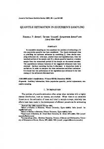
30

0.7

Average MAD estimate 0.9 0.8

1.0


0

20

40

60 Sample size

80

100

Figure 2.1: Average MAD estimates over one million replications of different sample sizes from a standard Gaussian distribution. The black line represents the finite sample correction factor and the grey line is the true parameter value.

The key difference between the MAD and the IQR is that the MAD possesses maximal asymptotic breakdown value, #⇤ = 0.5. For symmetric distributions, the MAD is asymptotically equivalent to onehalf of the interquartile distance. Hall and Welsh (1985), Welsh (1986) and more recently, Mazumder and Serfling (2009) study the asymptotic properties of the MAD and its link with the semi-IQR. With correction factors to ensure consistency for the standard deviation at the Gaussian distribution, the MAD can be redefined as, MAD( x) = bn 1.4826 ⇥ Med{| x

Med{ x}|},

(2.17)

where the bn factors are chosen to make MADn approximately unbiased in finite samples. Croux and Rousseeuw (1992) use simulation to find finite sample correction factors for the MAD. In particular, they specify them explicitly for 2  n  9 and if n > 9 then use the approximation, bn =

n . n 0.8

In R, the only correction implemented is an asymptotic one, i.e. bn = 1 for all n. The need for a finite correction factor is demonstrated in Figure 2.1.

31

2.4 a scale estimator based on pairwise means

2.3.2.7

t-scale

Yohai and Zamar (1988) introduce the class of t-estimates which have a high breakdown value and controllable efficiency at the Gaussian distribution. If sˆ ( x) is a robust M-estimator of scale, i.e. a solution of equation (2.13), then the t-scale is defined as, ✓ ◆ 1 n xi 2 2 t ( x) = sˆ ( x) Â r . n i =1 sˆ ( x) Maronna and Zamar (2002) propose a version of the t-scale that will be considered in Chapter 4. Namely, the initial M-estimator of scale is the MAD, sˆ ( x) = MAD( x). The t-scale estimate is, ✓ ◆ 1 n xi µˆ ( x) Ân w x 2 t ( x) = d MAD( x) Â rc1 , where µˆ ( x) = i=n1 i i . n i =1 MAD( x) Â i =1 wi Note that d is a asymptotic correction factor to ensure consistency at the Gaussian distribution, rc1 (v) = min(c21 , v2 ) with default c1 = 3 and the weights are calculated as, ✓ ◆ xi Med( x) wi = w c2 , MAD( x) where wc2 (u) = max(0, (1 2.4

(u/c2 )2 )2 ) and the default is c2 = 4.5.

a scale estimator based on pairwise means

2.4.1 The estimator Pn Given a set of n observations, x = ( x1 , . . . , xn ), the set of (n2 ) pairwise means is { g( xi , x j ), 1  i < j  n}, where g( x1 , x2 ) = ( x1 + x2 )/2. Let Gn be the empirical distribution function of the pairwise means, Gn (t) =

2 n(n

1) iÂ = (1 + t ) n ( n 1). 2 2 2 4 Setting m ⇡ n#⇤ , for large n we have,

(n

n#⇤ )(n

n#⇤

1) >

1 (1 + t )(n2 2

Thus, ⇤

# d, s( x)

(2.20)

where d is an arbitrary constant. Note that d needs to be sufficiently large such that not all the observations are trimmed. The metric on the left hand side of (2.20) is the absolute value of the generalised scaled deviation, as

36


defined in Wu and Zuo (2009). Simulations suggest a value of d = 5 represents a good trade off between achieving high efficiency at heavy tailed distributions whilst maintaining high efficiency at light tailed distributions. This is in agreement with Wu and Zuo (2009) who recommend a value for the tuning parameter of between 4 and 7. The estimator Pen will inherit its breakdown value from the minimum breakdown value of the preliminary estimates, #⇤ ( x, Pen ) = min{#⇤ ( x, m), #⇤ ( x, s)}.

Choosing estimators with 50% breakdown values, for example setting m( x) to be the median or Huber’s M-estimate of location and s( x) to be the MAD or Qn , translates to a 50% breakdown value for Pen . Adaptive trimming of the pairwise means is another alternative to the standard Pn statistic. Using auxiliary estimates of location and scale, each with a breakdown value of 50% to adaptively trim the kernels yields a pairwise mean scale statistic with a breakdown value of 0.29, the same as that for the Hodges-Lehmann estimate of location. 2.4.2 Properties of Pn This section considers some of the properties of Pn . We begin by finding the limiting value of Pn (t ) defined in (2.18) as n ! • and provide correction factors to ensure consistency for the standard deviation in large samples when the distribution of the underlying observations is Gaussian. We also show evidence of finite sample bias and suggest finite sample correction factors for Pn . By exploiting the generalised L-statistic structure of Pn (t ), we find the influence function and infer related properties such as the asymptotic efficiency and gross error sensitivity for Pn (t ). We also establish the asymptotic normality of Pn (t ). 2.4.2.1

Correction factors

As noted in (2.18), a correction factor, ct is required to ensure Pn (t ) is consistent for the standard deviation in the Gaussian case. Without loss of generality, let F, the distribution of the underlying observations, be centred at zero. The CDF of the pairwise means, ( X1 + X2 )/2, is given by, G (t) =

Z • Z 2t u •

•

f ( x ) f (u) dx du =

Z •

•

F (2t

u) f (u) du.

(2.21)

37


When the underlying data follow a Gaussian distribution with CDF, F, and density, F0 = f, (2.21) can be written as, GF (t) =

Z •

•

F(2t

x )f( x ) dx.

The correction factor for a given t 2 (0, 1) is, 1/ct = GF 1 ((1 + t )/2)

GF 1 ((1

t )/2).

(2.22)

The expression in (2.22) can easily be obtained using numerical integration. In particular for Pn , the corresponding asymptotic correction factor is, c0.5 = c ⇡ 1/0.9539 ⇡ 1.0483. The finite sample correction factors are applied after the large sample correction has been made. Finite sample correction factors for Pn , cn,0.5 , have been found analytically for n = 3 and 4: c3,0.5 = 1.13 and c4,0.5 = 1.30 (see Section B.1 in Appendix B for details). The finite sample correction factors exhibit jumps and are not monotonically increasing in n, instead they exhibit a periodic pattern attributable to the order statistic method used to find the quantiles. For 5  n < 40, finite sample correction factors have been found using simulation, a sample of these is given in Table B.1 in Appendix B. For n 40 the small sample correction factor for Pn is well approximated by cn,0.5 = n/(n 0.7). 2.4.2.2

Influence function

Noting that Pn (t ) is a GL-statistic and using equation (2.15) from Serfling (1984) we have the following result. Result 2.1. If F has derivative f > 0 on [ F influence function for Pn (t ) is, IF( x; Pn (t ), F ) = ct



1 ( e ), F 1 (1

e)] for all e > 0, the

(1 + t )/2 F (2G 1 ((1 + t )/2) x ) R f (2G 1 ((1 + t )/2) x ) f ( x ) dx (1 t )/2 F (2G 1 ((1 t )/2) x ) R . f (2G 1 ((1 t )/2) x ) f ( x ) dx

Figure 2.4 plots the influence functions for Pn , Qn , the MAD and the SD when the underlying data are Gaussian. Figure 2.4 shows that Pn has a gross error sensitivity of g⇤ = 2.33, slightly higher than that of Qn , g⇤ = 2.07 at the Gaussian distribution. As Hampel (1974) notes, the asymptotic variance of an estimator approaches its minimum as the influence function approaches a multiple of the log likelihood derivative. Hence, when the underlying observations are Gaussian, the closer an estimator’s influence function

38


2

MAD

0

Qn

1

Pn

1

IF( x; S, F )

SD

2

4

0 x

2

4

Figure 2.4: Influence functions of the SD, Qn , Pn and the MAD when the model distribution is Gaussian.

is to that of the SD, the more efficient it will be. In Figure 2.4 the influence function of Pn is almost always closer to that of the SD than Qn . This is reflected in our calculation of the asymptotic variance, which is found as the expected square of the influence function. Numerical integration yields, V=

Z

R

IF2 ( x; Pn , F) dF( x ) = 0.579.

(2.23)

This equates to an asymptotic efficiency of 0.86 as compared with 0.82 for Qn and 0.37 for the MAD at the Gaussian distribution. Thus, despite having a higher gross error sensitivity, Pn is a more efficient estimator than Qn at the Gaussian distribution. It is also important to consider efficiencies at distributions other than the Gaussian. If Y follows a Student’s t distribution, it can be generalised as a location-scale model, X = µ + sY, with density, ✓ ◆2 ! (n+1)/2 1 G ( n+ ) 1 x µ p2 f (x) = 1+ , n s G( n2 ) pns R• where G(z) = 0 x z 1 e x dx is the gamma function. It is important to note that in this setting s is a scale parameter, not the standard deviation, so it still exists and can be consistently estimated even when 1  n < 2. Setting µ = 0, Bachmaier (2000) adapts the work of Fisher (1922) to show that the Fisher information for the scale parameter of a scaled t distribution is,

I(s) =

2n . ( n + 3) s 2

39

0.9

Pn

0.6

0.7

0.8

Qn

0.5

MAD

0.4

Asymptotic relative efficiency

1.0


1

3 5 7 Degrees of freedom for the t distribution

9

Figure 2.5: Asymptotic relative efficiency of Qn , Pn and the MAD for t distributions with degrees of freedom ranging between 1 and 10.

Figure 2.5 shows the relative efficiency of Pn , Qn and the MAD at t distributions with degrees of freedom ranging between 1 (the Cauchy distribution) and 10 with scale parameter s = 1, i.e. standardised t distributions. The asymptotic relative efficiencies are calculated as the product of the inverse of the Fisher information and the asymptotic variance, calculated by replacing F in (2.23) with the CDF of the corresponding t distribution. It is clear from Figure 2.5 that t distributions with degrees of freedom more than approximately 2.5, Pn is more efficient than Qn . At extremely heavy tailed t distributions, including the Cauchy distribution, Qn is asymptotically more efficient than Pn . The MAD also performs better than Pn at the Cauchy, however its efficiency decays substantially as the degrees of freedom increase. At the exponential distribution the asymptotic relative efficiency of Pn to Qn is 0.77. Furthermore, the gross error sensitivity for Pn is g⇤ = 3.968 which compares with g⇤ = 2.317 for Qn at the exponential. However, it is not the case that Pn is necessarily worse than Qn for skewed distributions. When the underlying distribution of the data is c21 , the asymptotic relative efficiency of Pn to Qn is 1.43. The performance of Pn is more attractive than Qn for discrete distributions. In the limit, Qn will equal zero, and therefore fail to provide a valid estimate of scale, whenever more than 25% of the pairwise differences equal zero. For a discrete distribution with k distinct possible outcomes, x1 , x2 , . . . , xk , and

40


probability mass function P( X = x j ) = p j , for j = 1, 2, . . . , k, the expected proportion of pairwise differences equal to zero is Â j p2j . In particular,

Â p2j > 14 j

() lim P( Qn = 0) = 1. n!•

For example for the Poisson distribution with expected value 1, Â j p2j = 0.31 p

and hence Qn ! 0. In contrast, for Pn to return a scale estimate of zero, the IQR of the pairwise means must be equal to zero, that is, more than 50% of the pairwise means must be equal. Except for trivial two point distributions, we have shown that Pn = 0 implies Qn = 0 (see Section B.2 in Appendix B for details). The pairwise averaging process helps smooth the underlying discrete distribution which results in Pn being a better robust estimator than Qn in these situations. 2.4.2.3

Asymptotic normality

As defined in Section 2.2, let G (t) = P( g( X1 , X2 )  t) and Gn (t) be the CDF and empirical distribution function of a symmetric, bivariate U-statistic. This section proves the following result on the asymptotic normality of Pn (t ). Result 2.2. Let a = (1 t )/2, b = (1 + t )/2 for 0 < t < 1. If G has derivative G 0 > 0 on [ G 1 (b) #, G 1 ( a) + e] for some e > 0, then as n ! •,

p

where q = ct G

1 (b)

v( a, b) = 4

R

n( Pn (t )

G

1 ( a)

F (2G

D

q ) ! N (0, c2t V ),

, V = v( a, a) + v(b, b)

1 ( a)

2v( a, b), and

x ) F (2G 1 (b) x ) dF ( x ) G 0 ( G 1 ( a)) G 0 ( G 1 (b))

ab

.

To establish the limiting distribution, we note that Pn is a linear combination of two U-quantile statistics. Hence, we first consider the empirical U-process defined as,

p

n ( Gn (t)

G (t))

t 2R

.

p Silverman (1976, Theorem B) proves that in this context, n( Gn (·) G (·)) converges weakly in the Skorohod topology to an almost surely continuous, zero-mean Gaussian process, W, with covariance function, EW (s)W (t) = 4 P( g( X1 , X2 )  s, g( X1 , X3 )  t)

4G (s) G (t),

(2.24)

41

2.5 relative efficiencies in finite samples

for all s, t 2 R. Hence, for 0 < p < q < 1, if G 0 , the derivative of G, is strictly positive on the interval [ G 1 ( p) #, G 1 (q) + e] for some e > 0, then we can use the inverse map to show,

p ⇣ 1 n Gn (·)

G

1

(·)

⌘

W (G ! 0 G (G

D

1 (·)) 1 (·))

,

where W is a mean zero Gaussian process with covariance function defined in (2.24). See for example, van der Vaart and Wellner (1996, Section 3.9.4.2). Serfling (2002) summarises stronger results concerning empirical processes of U-statistic structure. For Pn (t ) we use the pairwise mean kernel, g( x, y) = ( x + y)/2. Conditioning on X1 = x the covariance function (2.24) can be rewritten as, cov(W (t), W (s)) = 4

Z

F (2s

x ) F (2t

x ) dF ( x )

4G (s) G (t),

where F is the distribution function of the underlying observations. The limiting covariance function for the quantiles used in the construction of Pn (t ), n cov( Gn 1 ( a), Gn 1 (b)), is, R F (2G 1 ( a) x ) F (2G 1 (b) x ) dF ( x ) ab v( a, b) = 4 , G 0 ( G 1 ( a)) G 0 ( G 1 (b)) for a = (1

t )/2, b = (1 + t )/2 and 0 < t < 1. Hence, p D n( Pn (t ) q ) ! N (0, c2t V ),

where q = ct G 1 (b) G 1 ( a) and V = v( a, a) + v(b, b) depend on F. Noting that the derivative of G (t) is, 0

G (t) =

Z

2 f (2t

u) f (u) du,

2v( a, b) both

(2.25)

it can be shown that the asymptotic variance found here is equivalent to the expected square of the influence function discussed previously. Furthermore, from the general results in Serfling (2002, Section 12.3.4), the almost sure behaviour of Pn (t ) can be deduced from the Bahadur representation for the U-quantiles. 2.5

relative efficiencies in finite samples

The asymptotic variance of Pn has been found and corresponding asymptotic efficiencies have been deduced in the previous section. In particular, it

42


has been shown that, asymptotically, Pn is more efficient than Qn for t distributions with more than approximately 2.5 degrees of freedom. However, it is often of practical interest to determine small sample relative efficiencies. This section considers the finite sample relative efficiency of Pn , and variants thereof, using configural polysampling. It also examines the finite relative efficiencies over the same range of t distributions considered asymptotically in Figure 2.5. 2.5.1 Design Under configural polysampling, estimators are evaluated at particular distributions chosen to exhibit more extreme characteristics than what might be observed in practice. For example, the Gaussian distribution has tails that die off rapidly, and the Cauchy has tails that die off extremely slowly. Such extreme distributions will be referred to as corners. If it can be shown that an estimator performs well over all the corners considered, it is a fair assumption that the estimator will perform at least as well at intermediate distributions. A key performance measure for estimators is the polyefficiency, the minimum efficiency that an estimator achieves over a selection of corners. Yatracos (1991) shows that high polyefficiency over a finite selection of corners implies at least as high an efficiency at any convex combination of these corners. Scale estimates are computed for samples of size n from each of Tukey’s three corners: the Gaussian corner where observations are sampled independently from a standard Gaussian distribution; the one wild corner, where n 1 observations are independent Gaussian and the remaining observation is scaled by a factor of 10; and the slash corner where observations are constructed as the ratio of an independent Gaussian random variable and an independent standard uniform random variable. The slash distribution has Cauchy-like tails, but is considered to be more generally representative of real data as it is less peaked at the median than the Cauchy. Improving on the methodology set out in Lax (1985), Randal (2008) proposes using MLEs as the benchmark against which all estimators are compared. Previously, efficiencies were typically measured relative to the most efficient estimator considered for each distribution. MLEs are asymptotically efficient and may be used as a common reference case in future simulation studies.

43


Kafadar (1982) gives the MLE for the slash distribution and Randal and Thomson (2004) describe how to find the MLE for the one wild distribution by nesting it within the class of Gaussian compound scale models and applying an EM algorithm. Randal (2008) demonstrates how to use a similar EM algorithm approach to find the MLE of scale for t distributions. These algorithms are not part of an R package, however, they are reasonably straightforward to implement and we include our R code in Appendix B.4. Efficiencies are estimated over m independent samples as, c (T) = eff

c (ln sˆ 1 , . . . , ln sˆ m ) var , c (ln S( x1 ), . . . , ln S( xm )) var

(2.26)

where for each j = 1, . . . , m, the x j are independent samples of size n, sˆ j is the scale MLE and S( x j ) is the proposed scale estimate. Rousseeuw and Croux (1993) propose an alternative efficiency measure, based on the standardised variances. This measure was also considered and gave results largely in agreement with the Lax relative efficiencies and are therefore not reported here. The key difference between these two measures of efficiency is the presence of a log transformation in (2.26) which acts to stabilise the variance estimates. This is not present in the alternative measure which therefore heavily penalises inefficient scale estimates in heavy tailed data. Correction factors do not play a role in determining efficiency in either measure. Therefore, so far as efficiency is concerned, it is not an issue that the estimators are defined with consistency factors for the standard Gaussian only. 2.5.2 Results Figure 2.6 presents the estimated relative efficiencies over t distributions with degrees of freedom ranging from 1 to 10 in increments of 0.5. The curves for Pn and Qn are similar to the asymptotic efficiencies in Figure 2.5. Of particular interest is the speed with which Pn overtakes the adaptively trimmed Pn . For t distributions with 2 or more degrees of freedom, Pn is more efficient than Pen , the adaptively trimmed form of Pn with tuning parameter d = 5. Furthermore, for t distributions with 3 or more degrees of freedom, Pn is more efficient than Qn . For skewed distributions, we obtain similar results in finite samples to what was observed asymptotically. In particular, the results are highly dependent on the type of skewed distribution. At the exponential, in samples of size n = 20, Pn is 0.87 times as efficient as Qn . Which is an improvement

44

0.9

Pn

0.8

Pen

0.5

0.6

0.7

Qn

0.4

Estimated relative efficiency

1.0


1

2

3 5 6 7 8 4 Degrees of freedom for the t distribution

9

10

Figure 2.6: Finite sample relative efficiency, estimated from one million t distributed samples of size n = 20, for Qn , Pn and adaptively trimmed Pn with tuning parameter d = 5, Pen .

over the asymptotic result. Whereas at the c21 distribution, in samples of size n = 20, Pn is 1.21 times more efficient than Qn . Figure 2.7 presents the relative efficiencies of a variety of scale estimators at Tukey’s three corner distributions in samples of size n = 20. The estimators considered are: Pn ; Pen , the adaptively trimmed Pn with tuning parameter d = 5; P˘n is symmetric fixed trimming where 5% of the observations have been trimmed off both tails of the original data, for n = 20 this means that the maximum and minimum values have been deleted; Qn and Sn (Rousseeuw and Croux, 1993); the MAD; and the IQR. The estimator Pn is observed to be the most efficient at the Gaussian and one wild corners, however, it performs poorly at the slash corner. Among the estimators considered, Pen with tuning parameter d = 5 has highest minimum efficiency across all three corners, therefore the estimator is known to be triefficient. Its lowest efficiency occurs at the one wild with 72%. However as noted in Figure 2.6, the efficiency gain from using Pen over Pn disappears as the tails become slightly less heavy. The triefficiencies over various sample sizes are reported in Table 2.2. The adaptively trimmed Pn with d = 5 is in fact triefficient over the range of sample sizes considered. While the triefficiencies of most estimators increases with sample size, those of the MAD and IQR do not, reflecting their exceptionally poor finite sample and asymptotic Gaussian efficiency.

45


Gaussian Pn Pen P˘n Qn Sn MAD IQR

One-wild Pn Pen P˘n Qn Sn MAD IQR

Slash Pn Pen P˘n Qn Sn MAD IQR

0.2

0.4

0.6

0.8

1.0

Estimated relative efficiency

Figure 2.7: Estimated efficiencies relative to maximum likelihood scale estimates for samples of size n = 20, calculated over one million independent samples. The various pairwise mean scale estimators are: Pn ; Pen , the adaptively trimmed Pn with tuning parameter d = 5; and P˘n is symmetric fixed trimming where 5% of the observations have been trimmed off both tails of the original data.

46


n

Gaussian 20

50

100

500

1000

0.853

0.854

0.862

0.860

0.858

0.819

0.850

0.861

0.860

0.858

0.566

0.678

0.725

0.753

0.757

0.718

0.747

0.730

0.726

0.724

Qn

0.677

0.737

0.778

0.809

0.812

MAD

0.376

0.368

0.374

0.365

0.363

IQR

0.396

0.375

0.376

0.366

0.362

Pn Pen with d = 5 Pen with d = 3 P˘n

n

One wild 20

50

100

500

1000

0.834

0.864

0.860

0.870

0.867

0.723

0.817

0.839

0.865

0.865

0.574

0.692

0.725

0.763

0.765

0.756

0.777

0.738

0.737

0.733

Qn

0.680

0.751

0.781

0.817

0.820

MAD

0.400

0.380

0.380

0.373

0.372

IQR

0.420

0.386

0.380

0.373

0.372


n

Slash 20

50

100

500

1000

0.480

0.626

0.703

0.773

0.786

0.748

0.785

0.809

0.833

0.829

0.766

0.799

0.809

0.822

0.826

0.665

0.738

0.820

0.876

0.886

Qn

0.945

0.950

0.959

0.961

0.963

MAD

0.876

0.851

0.847

0.837

0.844

IQR

0.839

0.830

0.839

0.839

0.843


Table 2.1: Estimated relative efficiencies relative to maximum likelihood scale estimates for the various scale estimators at each of Tukey’s three corners calculated over one million independent samples. Note that P˘n is symmetric fixed trimming where 5% of the observations have been trimmed off both tails of the original data.

47


20

50

100

500

1000

0.480

0.626

0.703

0.773

0.786

0.723

0.785

0.809

0.833

0.829

0.566

0.678

0.725

0.753

0.757

0.665

0.738

0.730

0.726

0.724

Qn

0.677

0.737

0.778

0.809

0.812

MAD

0.376

0.368

0.374

0.365

0.363

IQR

0.396

0.375

0.376

0.366

0.362

n Pn Pen with d = 5 Pen with d = 3 P˘n

Table 2.2: Triefficiencies of various scale estimators over a range of sample sizes.

Moderate amounts of fixed trimming, for example 5% at each tail as shown in Figure 2.7 does markedly improve the efficiency of Pn at the slash corner. However, it also compromises the efficiency of Pn at the Gaussian distribution. In other simulations we have conducted, this result is not noticeably improved as the sample size increases. Therefore, adaptive trimming with a sensible choice of the tuning parameter is recommended over fixed trimming. We have considered the impact that the tuning parameter d has on the efficiency of Pen . Intuitively, as d increases, more observations remain in the sample which, for distributions that are not extremely heavy tailed, tends to increase efficiency. However, if the data are sampled from an extremely heavy tailed distribution, in small samples the opposite tends be true – removing more of the observations in the tails actually increases the efficiency of the scale estimate. Table 2.1 shows that in samples of size n = 20 using an adaptive trimming parameter of d = 5 results in a Gaussian relative efficiency of 0.82, however using d = 3 results in a much lower Gaussian relative efficiency of 0.57. In contrast at the slash corner, d = 5 gives a slightly lower relative efficiency of 0.75 compared with the d = 3 of 0.77. As the sample size grows, the distinction between d = 5 and d = 3 is negligible at the slash corner, though at the Gaussian distribution using d = 5 results in a much more efficient estimator. From additional results not summarised in Figure 2.7 or Table 2.1, we find that random trimming of the kernels, i.e. the pairwise means, achieves similar results as randomly trimming the original data at the Gaussian and one wild corners, however, randomly trimming the original data leads to higher efficiency at the slash.

48

2.6 conclusion

The small sample performance of Pn is also better than the performance of Qn for discrete distributions. Consider, for example, the case of a binomial distribution, X ⇠ B(6, 0.4). In the limit neither Qn nor Pn will converge to zero. However, if samples of size n = 20 are drawn from this distribution, Qn will return a scale estimate of zero, on average 12% of the time due to the discrete nature of the data. In contrast, Pn returns zero less than 0.1% of the time. Apart from some trivial cases, if Pn = 0 in finite samples this implies that Qn = 0 (see Section B.2 in Appendix B for details). Importantly, Pn possesses comparable small sample efficiency to that obtained asymptotically. It performs particularly well at the Gaussian and one wild as well as heavy tailed distributions such as the t distribution with degrees of freedom greater than approximately 2.5. Even though Pen with a trimming parameter of d = 5 is triefficient amongst the scale estimators considered here, Pn would still be preferred as a scale estimator in small samples. As the sample size increases the efficiency of Pen with trimming parameter d = 5 approaches that of Pn at the Gaussian distribution and Pen remains quite efficient at the slash, indicating that a mild amount of adaptive trimming could be a worthwhile thing to do. The utility of an adaptively trimmed version of Pn is revisited in Chapter 4. 2.6

conclusion

This chapter details the scale estimator, based on the difference of two order statistics of the empirical distribution function of the pairwise means. Hence Pn (t ) fits into the GL-statistic framework, alongside many other well known scale estimators. Choosing t = 0.5 results in the estimator Pn which possesses reasonable robustness properties, whilst maintaining high efficiencies at Gaussian distributions and has an intuitive interpretation: the IQR of the pairwise means. We have found that Pn , in its standard form, has a breakdown value of 13%. Its influence function more closely approximates that of the SD at the Gaussian distribution, leading to a relatively high asymptotic efficiency of 86%. We have also found the gross error sensitivity and demonstrated the asymptotic normality of Pn . Furthermore, when the underlying distribution is discrete, Pn is more robust to repeated observations than Qn . In finite samples, Pn also performs admirably. In samples of size n = 20, at the Gaussian distribution, Pn is 27% more efficient than Qn and 22% more

49

2.6 conclusion

efficient at the one wild corner. Pn maintains its efficiency advantage over Qn even when the underlying distribution of the data has quite heavy tails. To summarise, Pn is a simple and intuitive robust scale estimator, that is not tailored to be most efficient at any particular distribution, rather it maintains high efficiency over a wide range of distributions.

50

C O VA R I A N C E A N D A U T O C O VA R I A N C E E S T I M AT I O N

3.1

introduction

Motivated by the potential to extend the efficiency and robustness properties of Pn to the time series setting, this chapter considers the problem of estimating scale and autocovariance in dependent processes. We begin by considering a general device commonly used to extend scale estimators to the covariance setting, before outlining the properties of the resulting covariance estimator when Pn is used as the underlying scale estimator. Standard results are used to show that the asymptotic efficiency and robustness properties carry through and simulation results are provided for the robust correlation coefficient. We also discuss some of the implications for robustness when the covariance estimator is used in a time series setting as an autocovariance estimator. The properties of the scale estimator Pn and the resulting autocovariance estimator under both short and long range dependent Gaussian processes are discussed. Standard asymptotic results are found to hold in the short range dependent (SRD) setting. In the long range dependent (LRD) setting we establish the asymptotic normality of Pn under short and mildly long range dependent Gaussian processes. Under extreme long range dependence, we motivate a complication in establishing the limiting distribution for Pn by first proving a non-Gaussian limit result for the IQR, consistent with results for other common scale estimators, such as the SD and Qn . In contrast with the results of Lévy-Leduc et al. (2011c) for a single U-quantile, namely Qn , the proof for the IQR, a difference of two quantiles, relies on the higher order terms in the Bahadur representation of Wu (2005). Furthermore, we posit that Pn , the IQR of the pairwise means, has a similar behaviour, though the proof relies on an analogous conjectured Bahadur representation for U-quantiles under long range dependence. The asymptotic results for the robust scale estimator extend to the corresponding robust autocovariance estimators. Our theoretical results are illustrated with simulations.

51

3

3.2 robust covariance estimation

Most of the literature concerning robust covariance estimation is focussed on the multivariate setting, i.e. estimating covariance or dispersion matrices. This topic will be addressed in Chapter 4. 3.2

robust covariance estimation

A simple method for turning scale estimators into covariance estimators was introduced by Gnanadesikan and Kettenring (1972) and brought to prominence in the context of robust estimation by Ma and Genton (2000, 2001). The idea is based on the identity, cov( X, Y ) =

1 [var(aX + bY ) 4ab

var(aX

bY )] ,

(3.1)

where X and Y are random variables. In general, X and Y may have different p p scales, hence it is standard to let a = 1/ var( X ) and b = 1/ var(Y ). A robust covariance estimator is found by replacing the variance in (3.1) with (squared) robust scale estimators. A nice feature of (3.1) is that it is location free, in the sense that no location parameter needs to be estimated when the robust scale estimator is also location free, such as Qn , IQR or Pn . The covariance estimator based on Pn is obtained by replacing the variance terms in (3.1) with the square of Pn , i 1 h 2 gP ( X, Y ) = Pn (aX + bY ) Pn2 (aX bY ) , (3.2) 4ab where a = 1/Pn ( X ) and b = 1/Pn (Y ). The correlation could also be estimated as, Pn2 (aX + bY ) Pn2 (aX bY ) , 4abPn ( X ) Pn (Y )

however this estimator does not necessarily satisfy the Cauchy-Schwarz inequality and so the estimated correlation coefficient would not necessarily lie in the range [ 1, 1]. To ensure that the estimated correlation coefficient lies in the appropriate range, Gnanadesikan and Kettenring (1972) propose using an estimator of the form, r P ( X, Y ) =

Pn2 (aX + bY ) Pn2 (aX Pn2 (aX + bY ) + Pn2 (aX

bY ) . bY )

While the covariance given by (3.2) depends on the correction factor built into the Pn estimator to ensure consistency at the Gaussian distribution, see equation (2.19), the correlation is independent of the choice of correction factor.

52


An advantage of covariance estimates based on the Gnanadesikan and Kettenring device, applying equation (3.1), is that the statistical properties of the resulting estimator are relatively straightforward to derive. 3.2.1 Properties Genton and Ma (1999) explore the robustness properties of dispersion estimators constructed using the identity (3.1). In the general case, let Sn ( Fn ) be a scale estimator with corresponding statistical functional S( F ). Let gS be a statistical functional of covariance corresponding to a covariance estimate gˆ S based on (3.1), i 1 h 2 gS ( F ) = S ( F+ ) S2 ( F ) , 4ab

where F is a bivariate distribution with marginal distributions FX and FY , and F± denotes the distribution of aX ± bY with scale s± respectively. 3.2.1.1

Influence function

Genton and Ma (1999) show that the influence function of gS can be defined in terms of the influence function of S as follows, 1 ⇥ IF( x, y; gS , F ) = S( F+ ) IF(ax + by; S, F+ ) 2ab ⇤ S( F ) IF(ax by; S, F ) . (3.3)

Note that this formulation of a bivariate influence function in terms of two univariate influence functions requires the unidimensional Dirac function dx be generalised to a bidimensional Dirac function where the perturbations depend on the choice of the covariance estimator, i.e. along the ax + by and ax by directions. Since a and b are arbitrary non-zero constants, we p can simply set a = 1/sX and b = 1/sY , where sX = var( X ) and sY = p var(Y ), in which case (3.3) can be rewritten as,  ✓ ◆ sX sY x y IF( x, y; gS , F ) = s+ IF + ; S, F+ 2 sX sY ✓ ◆ x y s IF ; S, F . (3.4) sX sY

Ma and Genton (2001) use the general form, (3.4), to state the influence function for covariance estimators based on Qn ,  ✓ ◆ ✓ ◆ sX sY x y x y IF( x, y; gQ , F ) = s+ IF + ; Q, F+ s IF ; Q, F , 2 sX sY sX sY

53


where F± is the distribution function of sXX ± sYY respectively, and the influence function for Qn is given in (2.11). We can similarly use the general form, (3.4), to find the influence functions for the covariance estimator based on Pn ,  ✓ ◆ ✓ ◆ sX sY x y x y IF( x, y; gP , F ) = s+ IF + ; P, F+ s IF ; P, F . 2 sX sY sX sY The influence function for Pn (t ) has been found previously in Result 2.1. For Pn = Pn (0.5) this simplifies to, " # 3 1 F (2G 1 ( 34 ) x ) F (2G 1 ( 14 ) x ) 4 4 R IF( x; P, F ) = c R . f (2G 1 ( 34 ) x ) f ( x )dx f (2G 1 ( 14 ) x ) f ( x )dx

We will focus specifically on Gaussian processes, in which case, Z

f(2GF 1 ( 34 )

Z

f(2GF 1 ( 41 ) x )f( x )dx p p = f( 2GF 1 ( 34 ))/ 2.

x )f( x )dx =

Hence we have, IF( x; P, F) = c

"

1 2

F(2GF 1 ( 34 ) x ) + F(2GF 1 ( 14 ) p p f( 2GF 1 ( 34 ))/ 2

x)

#

.

(3.5)

Importantly, the influence function of the covariance estimator is bounded and hence, the covariance estimator based on Pn is B-robust, i.e. has finite gross error sensitivity. 3.2.1.2

Asymptotic variance

As with scale estimators, the asymptotic variance of covariance and correlation estimators can be found as the expected square of the influence function (Hampel et al., 1986). Furthermore, if the scale estimator S is consistent and asymptotically normally distributed, then the covariance estimator, gS will also be consistent and asymptotically normal with asymptotic variance given by: n

1

V ( gS , F ) =

Z

IF2 ( x, y; gS , F ) dF ( x, y).

Genton and Ma (1999) show that the asymptotic variance of dispersion estimators is directly proportional to that of the underlying scale estimator. This reinforces the importance of using a highly efficient scale estimator,

54


V ( gS , F r ) gMAD

5 4 3

gP gSD

2 1 1

1

r

Figure 3.1: Asymptotic variance of covariance estimators, gS , based on various scale estimators at the bivariate Gaussian distribution over a range of correlations 1  r  1.

the efficiency benefits carry through to covariance estimation. In particular, restricting attention to bivariate Gaussian distributions, Fr , V (gS , Fr ) = 2(1 + r2 )V (S, F),

(3.6)

p where V (S, F) is the asymptotic variance of nS at F. p The asymptotic variance for nPn at the Gaussian distribution has previously been shown, in (2.23), to be V ( P, F) = 0.579 which compares with V (SD, F) = 0.5, V ( Q, F) = 0.61 and V (MAD, F) = 1.35. This results in a modest increase in asymptotic variance for gP over gSD as shown Figure 3.1. Indeed, given that the asymptotic variance of covariance (and correlation) estimators is directly proportional to that of the underlying scale estimator, the asymptotic efficiency of gP and r P compared to the classical covariance estimator at the Gaussian distribution is 86%, the same as that of Pn regardless of the level of correlation in the underlying bivariate Gaussian distribution. 3.2.1.3

Breakdown value

The notion of a breakdown value needs to be reinterpreted slightly in the context of (3.1). Ma and Genton (2000) define the breakdown value for a | | covariance estimator as follows. Let x = ( x1 , . . . , xn ) and y = (y1 , . . . , yn ) e be obtained by replacing be two samples of size n. Let Z = [ x, y] and let Z

55


e are then referred to any m pairs of Z by arbitrary values. The columns of Z as xe and ye. The sample breakdown point of a covariance estimator, gˆ S ( Z ) =

1 h 2 S (ax + by) ab n

i by) ,

Sn2 (ax

based on a scale estimator Sn is, ( m ⇤ e ) < • and inf gˆ S ( Z e) > # (gˆ S ( Z )) = max : sup gˆ S ( Z n e Z e Z

inf Sn (ae x + bye) > 0 and inf Sn (ae x e Z

e Z

• and bye) > 0 .

Hence, the breakdown value of gP is 13.4%, inherited directly from Pn (see Section 2.4 for details). To see that this is indeed the case, let xi (or yi ) be contaminated, then so too is axi ± byi . Hence if we consider the observations as pairs ( x1 , y1 ), . . . , ( xn , yn ), then at most 13.4% of the observed pairs can contain contaminated data before the Pn estimator breaks down, and hence gP breaks down. 3.2.2 Simulations Having established some asymptotic efficiency results for the covariance estimator at the Gaussian distribution and shown that the robustness and efficiency properties do indeed flow through from the univariate to the bivariate case, we now present some finite sample results for the correlation estimates when the underlying data follows a bivariate t distribution. There are a number of ways to define a multivariate t distribution, see Kotz (2004) for a recent summary. The form considered in this section is the most common and natural generalisation of the univariate t distribution. A p-dimensional random vector is said to follow a p-variate t distribution with mean vector µ, correlation matrix R and n degrees of freedom if its joint probability density function is given by,  1 G((n + p)/2) f ( x) = 1 + (x n (pn) p/2 G(n/2)| R|1/2

|

µ) R

1

(x

(n+ p)/2

µ)

.

As scale and covariance is the primary feature of interest, without loss of generality, we will restrict attention to the central multivariate t distribution where µ = 0. Note that in this setting, if p = 1 and R = 1 then we recover the univariate t distribution. Furthermore, as n ! • we recover the multivariate Gaussian distribution.

56


In the simulations that follow, the robust estimates are compared to the (non-robust) MLE calculated assuming that the degrees of freedom parameter is known. This is consistent with how the simulations were performed in Section 2.5, to give a reproducible base line for future comparisons. The MLE of the multivariate t was calculated in R using the cov.trob function from the MASS package (Kent, Tyler and Vard, 1994; Venables and Ripley, 2002). Comparisons are only made for n > 3 as the MLE covariance estimates are unstable for 1  n < 3. Indeed for n  2 we would be estimating a scatter matrix, which is defined more generally than a covariance matrix, as second order moments no longer exist, even though the density of a multivariate t distribution is still well defined for all n > 0. Figure 3.2 shows the efficiency of various scale estimates relative to the MLE for bivariate t distributions with correlation equal to 0.5 over a range of degrees of freedom. Over the observed range of degrees of freedom, r P is consistently more efficient than the other robust methods. As the degrees of freedom increase, the efficiency of the non-robust SD based method, rSD , increases and will approach parity with the MLE as n ! •. Most of the robust estimators exhibit a slight downward trend in their relative efficiency as the degrees of freedom parameter increases, however r P is reasonably invariant to changes in the degrees of freedom over the range considered here. As expected, rMAD performs substantially worse than similar estimates based on Pn and Qn and the minimum covariance determinant (MCD) methods are even less efficient. Figure 3.3 shows the relative mean square errors (MSEs). There is no discernible difference between the pattern of efficiencies in Figure 3.2 and the pattern of MSEs in Figure 3.3 indicating that any potential bias introduced by using robust estimators is negligible. This is to be expected, given the correction factors used in the underlying scale estimators cancel when the correlations are calculated. Figure 3.4 considers what happens to the relative efficiencies of the robust estimators as the level of dependence increases. For all estimators, efficiency appears to decrease as the level of dependence increases while keeping the degrees of freedom parameter fixed at n = 5. As the dependence level increases, it appears that the MLE does a better job than the robust measures of utilising what information is available information than the robust measures, potentially as a result of the decrease in effective iid sample size. Regardless of the level of dependence r P remains substantially more efficient than rQ . In Figure 3.2, r P is more efficient than rSD when n = 5 with correl-

57

1.0


SD

Relative efficiency 0.4 0.6 0.8

Pn Qn MAD

0.2

MCD

3


10

1.0

Figure 3.2: Estimated relative efficiencies for the correlation estimates over N = 100, 000 samples of size n = 20 from bivariate t distributions with correlation equal to 0.5. The efficiencies are measured relative to the MLE with known degrees of freedom.

SD

Relative MSE 0.8 0.6 0.4

Pn Qn MAD

0.2

MCD

3


10

Figure 3.3: Estimated relative MSEs for the correlation estimates over N = 100, 000 samples of size n = 20 from bivariate t distributions with correlation equal to 0.5. The efficiencies are measured relative to the MLE with known degrees of freedom.

58


ation equal to 0.5. Figure 3.4 shows that the same is true regardless of the level of dependence. Furthermore, it appears again that there is negligible bias present in the robust covariance estimators, as indicated by the agreement between the relative MSEs in Figure 3.5 with the relative efficiencies in Figure 3.4.

59

1.0


Pn

Relative efficiency 0.4 0.6 0.8

SD

Qn MAD

0.2

MCD

0.0

0.2

0.4 Correlation

0.6

0.8

1.0

Figure 3.4: Estimated relative efficiencies for correlation estimates over N = 100, 000 samples of size n = 20 from bivariate t distributions with n = 5 degrees of freedom and correlations ranging from 0 to 0.9. The efficiencies are measured relative to the MLE with known degrees of freedom.

Pn

Relative MSE 0.8 0.6 0.4

SD

Qn MAD

0.2

MCD

0.0

0.2

0.4 Correlation

0.6

0.8

Figure 3.5: Estimated relative MSEs for correlation estimates over N = 100, 000 samples of size n = 20 from bivariate t distributions with n = 5 degrees of freedom and correlations ranging from 0 to 0.9. The efficiencies are measured relative to the MLE with known degrees of freedom.

60

3.3 robust autocovariance estimation

3.3

robust autocovariance estimation

In this section we will consider the problem of estimating scale and autocovariance in a time series setting. This is an important problem that has many applications including financial data, hydrology, quality control, and signal processing. To ensure that the quantities we are aiming to estimate do not change over time, we will restrict attention to time series observations, { Xi }i 1 , that satisfy the hypothesis of second-order stationarity: a. E ( Xi ) = µ for all i = 1, 2, . . .; b. var( Xi2 ) = s2 < • for all i = 1, 2, . . .; and c. cov( Xi+h , Xi ) = g(h) for all i, h 2 Z. Applying the identity from Gnanadesikan and Kettenring (1972) in a time series setting we can construct robust autocovariance estimators based on equation (3.1). That is, autocovariance estimators based on the identity, g(h) =

1 [var( X1 + Xh+1 ) 4

var( X1

Xh+1 )] .

(3.7)

The autocovariance at a particular lag, h, measures the degree of second order variation between observations that are a fixed distance, h, apart. Let x a:b = ( x a , . . . , xb ) denote a sequence of b a + 1 observations. In the simplest case we can substitute a standard (non-robust) estimate of the sample variance, 1h 2 sˆ (x 4 n h 1:n 1 n h = ( xi n h iÂ =1

gˆ sˆ (h) =

h + x h+1:n )

x¯1:n

sˆ n2

h )( xi + h

where sˆ n2 ( xn ) =

1 n ( xi n iÂ =1

h ( x1:n

h

x¯ h+1:n ),

xh+1:n )

i

0hn

1,

(3.8)

x¯1:n )2

and x¯ a:b = (b a + 1) 1 Âib= a xi . The resulting estimator (3.8) is asymptotically equivalent to the classical autocovariance estimator. Ma and Genton (2000) suggest a robust alternative by plugging in Qn , gˆ Q (h) =

1h 2 Qn 4

h ( x1:n h

+ xh+1:n )

Q2n h ( x1:n h

i

xh+1:n ) .

61


In an attempt to improve the efficiency whilst maintaining a level of robustness, we propose a similar autocovariance estimator based on Pn , i 1h 2 gˆ P (h) = Pn h ( x1:n h + xh+1:n ) Pn2 h ( x1:n h xh+1:n ) . (3.9) 4

In contrast to scale estimators, autocovariance estimators are not invariant to permutations of the underlying observations – which complicates the characterisation of their breakdown values. Ma and Genton (2000) reinterpret the breakdown point of a covariance estimator, as defined in Section 3.2.1.3, to incorporate the importance of temporal disturbances on autocov| ariance estimators. Let x = ( x1 , . . . , xn ) be a time series of length n. Let xe be obtained by replacing any m observations of x by arbitrary values. Denote Im a subset of size m of {1, . . . , n}. The temporal sample breakdown point of an autocovariance estimator gˆ (h) is: ( m #⇤ (gˆ (h)) = max : sup sup Sn h (ue) < • and inf inf Sn h (ue) > 0 and n Im xe Im xe ) sup sup Sn Im

xe

e) h (v

< • and inf inf Sn Im

xe

e) h (v

>0

where ue = xe1:n h + xeh+1:n , ve = xe1:n h xeh+1:n . This definition highlights the importance of the positioning of the corruption taken into account through the supremum and infimum on the set of arrangements, Im . The breakdown value represents the worst case scenario. A particular example of this is given in Figure 3.6 which considers the autocovariance at lag h = 2 from a sample of size n = 13. The autocovariance estimator works with the data sets, x1:11 ± x3:13 . If four observations are contaminated in an appropriate way so as to cause maximum damage, this will h=2 X1

X2

X3

X4

X5

X6

X7

X8

X9

X10 X11 X12 X13

X1

X2

X3

X4

X5

X6

X7

X8

X9

X10 X11 X12 X13

h=2 Figure 3.6: Illustration of the effect of contamination on autocovariance estimators. The black observations have been contaminated. If appropriately arranged, the contamination of four observations leads to eight pairs of observations being contaminated.

62


result in 8 contaminated pairs. Ma and Genton (2000, Proposition 1) show that asymptotically the breakdown value for autocovariance estimators is half that of the corresponding covariance estimator. Hence, the asymptotic breakdown value for gˆ P is 6.7%. The influence function for the autocovariance estimator has the same general form as in the covariance case, (3.4). Importantly, the influence function of gˆ P remains bounded and as such the estimator has finite gross error sensitivity. In the remainder of this chapter, attention will focus on Gaussian processes hence an important special case of (3.4) is given by, ! x+y IF( x, y; gP , Fr ) = (g(0) + g(h)) IF p ; P, F 2(g(0) + g(h)) ! x y (g(0) g(h)) IF p ; P, F , (3.10) 2(g(0) g(h))

where the influence function of Pn at F is defined in (3.5). The asymptotic distribution and efficiency properties of Pn and gˆ P depend on the level of dependence in the underlying time series. The influence functions are a key ingredient when it comes to proving limit results for gˆ P under short and long range dependent Gaussian processes in Sections 3.4 and 3.5. The results under SRD follow closely what has been done by Lévy-Leduc et al. (2011c) for gˆ Q . However, in the LRD setting, some novel results are found and conjectures drawn that contrast with the limiting distribution of the Hodges-Lehmann estimator established by Lévy-Leduc et al. (2011a). These somewhat surprising results follow as Pn , the difference of two Uquantile statistics, has a distinct asymptotic behaviour to that of the individual U-quantiles. Furthermore, we observe the same limiting behaviour for a number of robust scale and autocovariance estimators under a certain type of LRD process. We show that the limiting result for the IQR is the same as that for Qn and the SD and we conjecture that the same is true for Pn and the MAD. We also show how the results for the autocovariance estimators follow from the results for the underlying scale estimators.

63

3.4 short range dependent gaussian processes

3.4

short range dependent gaussian processes

A sequence of observations whose autocovariance function is summable is known as a short range dependent (SRD) time series and is said to have short memory. Formally, let { Xi }i 1 be a stationary time series and let gh be its autocovariance function at lag h. The sequence { Xi }i 1 is said to be of short memory if Âh 1 |gh | < •. Assumption 3.1. { Xi }i 1 is a stationary mean-zero Gaussian process with autocovariance sequence g(h) = E ( X1 Xh+1 ) satisfying Âh 1 |g(h)| < •. The asymptotic normality for Pn and gˆ P under the conditions outlined in Assumption 3.1 is established in this section. We follow the same general approach that Lévy-Leduc et al. (2011c) use to establish similar results for Qn . The derivation is a little more involved, owing to the nature of Pn as a difference of two U-quantiles, rather than a single U-quantile as is the case for Qn . 3.4.1 Results for Pn Before considering the asymptotic distribution of the autocovariance estimator gˆ P , we first need results regarding the underlying scale estimator, Pn . This section is dedicated to the proof of the following result regarding the asymptotic distribution of the scale estimator Pn under SRD Gaussian processes. Result 3.1. Under Assumption 3.1, Pn satisfies the following central limit theorem (CLT): p D n( Pn s ) ! N (0, e s 2 ), p where s = g(0) and the limiting variance e s2 is given by  ✓ ◆  ✓ ◆ ✓ ◆ X1 Xk +1 2 2 2 X1 2 e s = s E IF ; P, F + 2s Â E IF ; P, F IF ; P, F . s s s k 1

The proof of Result 3.1 requires the following structure. Let I be a compact interval of R and let D( I ) be the space of all functions that are right continuous and whose limits from the left exist everywhere on I, i.e. the set of càdlàg functions. Let M([ •, •]) be the set of CDFs on [ •, •]. Equip both D and M with the topology of uniform convergence and denote the uniform norm by || · ||• .

64


We need to define functionals in terms of the underlying distribution. First the pairwise mean mapping, T1 :

M([ •, •]) ! D([ •, •])

F 7 ! r 7 ! G (r ) =

Secondly the quantile mappings,

RR

I { x + y  2r }dF ( x )dF (y) .

D([ •, •]) ! R

T2 :

G 7! G

1 1 ( 4 ),

and,

D([ •, •]) ! R

T3 :

G 7! G

1 3 ( 4 ).

Finally we need the lower and upper quartiles of the pairwise means,

M([ •, •]) ! R

T1 :

TL = T2

F 7! G

1 1 ( 4 ),

and, TU = T3

M([ •, •]) ! R

T1 :

F 7! G

1 3 ( 4 ).

The scale estimator Pn can now be expressed as, Pn = c [ TU ( Fn )

TL ( Fn )] = c ( TU

TL ) ( Fn ),

which is a consistent estimator of, P(Fs ) = c( TU

TL )(Fs ) = s,

where Fs is a Gaussian distribution with mean zero and variance s2 . Recall that the correction factor c = 1.0483, defined in Section 2.4.2.1, ensures Pn is consistent for the standard deviation at the Gaussian distribution. For the remainder of this chapter, without loss of generality, let s = 1 and P ( F ) = P ( F1 ). The proof begins by showing that T1 , T2 and T3 and consequently TU and TL are Hadamard differentiable2 defined continuously on D( I ). We then 2 Refer to Section C.1 in Appendix C (p. 151) for a definition of Hadamard differentiability.

65


express the estimator Pn as a sum of influence functions with an asymptotically negligible remainder term. A CLT for the sum of influence functions gives the required result. To show that T1 is Hadamard differentiable, let { gt } 2 D( I ) be a sequence of càdlàg functions with bounded variations such that || gt g||• ! 0 as t ! 0, where g is also a càdlàg function. Now for any r 2 R, consider T1 ( F + tgt )[r ] t

T1 ( F )[r ]

1

=t =2

RR

Furthermore,

RR

⇥R R

I { x + y  2r } dF ( x ) dgt (y) RR +t I { x + y  2r } dgt ( x ) dgt (y).

I { x + y  2r } dF ( x ) dgt (y)

=

Z Z 2r x R

 2|| gt

I { x + y  2r } d[ F + tgt ]( x ) d[ F + tgt ](y) RR ⇤ I { x + y  2r } dF ( x ) dF (y)

•

RR

I { x + y  2r } dF ( x ) dg(y) Z Z 2r x

dgt (y) dF ( x )

g||• ! 0

R

•

dg(y) dF ( x )

as t ! 0.

Hence, the Hadamard derivative of T1 at g is given by, T ( F + tgt )[r ] (Dg T1 ( F ))[r ] = lim 1 t !0 t

T1 ( F )[r ]

=2

Z Z 2r x R

•

dg(y) dF ( x ),

where Dg is the Hadamard derivative operator. The inverse mappings T2 and T3 are shown to be Hadamard differentiable in van der Vaart (1998, Lemma 21.3) and also van der Vaart and Wellner (1996, Lemma 3.9.20). Applying the chain rule for the inverse map, van der Vaart (1998, Theorem 20.9), we have, Dg TL ( F ) = Dg ( T2

T1 )( F ) =

=

(Dg T1 ( F ))[ TL ( F )] ( T1 ( F ))0 [ TL ( F )] R R 2T ( F) x 2 R •L dg(y) dF ( x ) . ( T1 ( F ))0 [ TL ( F )]

(3.11)

Similarly, Dg TU ( F ) = Dg ( T3

T1 )( F ) =

2

R R 2TU ( F) R

•

x

dg(y) dF ( x )

( T1 ( F ))0 [ TU ( F )]

.

(3.12)

66


Hence, Dg ( TU TL )( F ) is a continuous function of g and is defined on D( I ), and as such ( TU TL )( F ) is Hadamard differentiable. If for some sequence of numbers an ! • we have an ( Fn F ) converging in distribution, then we can apply the functional delta method of van der Vaart (1998, Theorem 20.8), to write, an ( Pn

P) = an c( TU

= c D{an ( Fn

TL )( Fn

F)

F )} ( TU

TL )( F ) + o p (1).

(3.13)

When F = F, under the conditions of Assumption 3.1, we can apply Csörgó p and Mielniczuk (1996) to show that n( Fn F) converges in distribution p to a Gaussian process in D( I ). Hence, (3.13) is valid with an = n. Using the results in (3.11) and (3.12) we have, i p h D{pn( Fn F)} ( TU TL )(F) = n D{ Fn F} ( TU )(F) D{ Fn F} ( TL )(F)  R p ( Fn F)(2TU (F) x ) dF( x ) =2 n ( T1 (F))0 [ TU (F)] R ( Fn F)(2TL (F) x ) dF( x ) + ( T1 (F))0 [ TL (F)] p = 2 n [ A An ] , where,

R

R

R

R

F(2TU (F) x ) dF( x ) A= R ( T1 (F))0 [ TU (F)] and,

Fn (2TU (F) x ) dF( x ) An = R ( T1 (F))0 [ TU (F)]

R

F(2TL (F) x ) dF( x ) , ( T1 (F))0 [ TL (F)]

x ) dF( x ) R Fn (2TL ( F ) . 0 ( T1 (F)) [ TL (F)]

Note that the numerators in A can be simplified, A=

3/4 ( T1 (F))0 [ TU (F)]

1/4 . ( T1 (F))0 [ TL (F)]

The numerators in An can be rewritten as, 1 n F(2TU (F) n iÂ =1

Xi )

and

1 n F(2TL (F) n iÂ =1

Xi ) .

Noting the symmetry in TU and TL we have, 0 ( T1 (F))0 [ TU (F)] = ( T1 (F))0 [ TL (F)] = GF ( TU (F))

Z

= 2 f(2TU (F) x )f( x )dx p p = 2f( 2TU (F)).

67


Hence, from (3.13) we have that, p n( Pn P) = c Dpn( Fn F) ( TU TL )(F) + o p (1) " c n 12 F(2TU (F) Xi ) + F(2TL (F) p p =p Â n i =1 f( 2TU (F))/ 2

Xi )

#

+ o p (1)

c n = p Â IF( Xi ; P, F) + o p (1), n i =1

(3.14)

where the influence function for Pn at the Gaussian distribution was given in (3.5). A CLT for n 1/2 Âin=1 IF( Xi ; P, F) follows from Arcones (1994, Theorem 4).3 Hence, under Assumption 3.1,

where

1 n D p Â IF( Xi ; P, F) ! N (0, e s 2 ), n i =1

h i e s2 = E IF2 ( X1 ; P, F)2 + 2

Â E [IF(X1; P, F) IF(X1+k ; P, F)] .

k 1

p Result 3.1, where observations have standard deviation, s = g(0), follows by noting that IF( x; S, Fs ) = s IF( x/s; S, F) from Proposition C.1 in Appendix 3 (p. 151). 3.4.2 Results for gˆ P (h) Having established the limiting distribution of the scale estimator, Pn , it is relatively straightforward to find the limiting distribution of the autocovariance function gˆ P . This section proves the following result regarding the asymptotic distribution of the autocovariance estimator gˆ P under SRD Gaussian processes. Result 3.2. Under Assumption 3.1, gˆ P (h) satisfies the following CLT,

p

n(gˆ P (h)

D

g(h)) ! N (0, s˘ 2 (h)),

where h i s˘ 2 (h) = E IF2 ( X1 , X1+h ; gP , Fr ) ⇥ ⇤ + 2 Â E IF( X1 , X1+h ; gP , Fr ) IF( Xk+1 , Xk+1+h ; gP , Fr ) k 1

and IF( x, y; gP , Fr ) is defined in equation (3.10). 3 See Section C.3 in Appendix C (page 158) for details. In particular, we show that the Hermite rank of the influence function equals 2.

68


Let F+ and F denote the CDFs of { Xi + Xi+h }i 1 and { Xi Xi+h }i 1 , respectively. Similarly let F+,n h and F ,n h denote the empirical distribution functions of { Xi + Xi+h }1in h and { Xi Xi+h }1in h . Also let P±,n h = Pn2 h ( x1:n h ± xh+1:n ). Since the underlying Gaussian process, { Xi }i 1 , satisfies the SRD assumptions, the same holds for { Xi + Xi+h }i 1 and { Xi Xi+h }i 1 . Furthermore, with the appropriate correction factor we have that p P(F± ) = 2(g(0) ± g(h)) and hence, g(h) =

P2 ( F + )

P2 ( F )

4

.

p We apply Csörgó and Mielniczuk (1996) to show that n h( F±,n h F± ) converges in distribution to Gaussian processes in D( I ). Thus, using a similar argument to above, p

n

h ( P±,n

h

P(F± )) = p

n h 1 Â IF(Xi ± Xi+h ; P, F± ) + o p (1). n h i =1

Using the functional delta method, van der Vaart (1998, Theorem 3.1), with b( x ) = x2 and b0 ( x ) = 2x, we obtain

p

n

h

⇣

2 P± ,n h

⌘

2P(F± ) n h P (F± ) = p Â IF(Xi ± Xi+h ; P, F± ) + o p (1). n h i =1 2

Applying the basic properties of influence functions, outlined in Proposition C.1 (p. 151), we have that, ! X1 ± X1 + h P(F± ) IF( X1 ± X1+h ; P, F± ) = 2(g(0) ± g(h)) IF p ; P, F . 2(g(0) ± g(h)) Hence, recalling from (3.10) that, 1h 2 gˆ P (h) = P (x + xh+1:n ) 4 n h 1:n h

Pn2

h ( x1:n

xh+1:n )

h

has influence function,

IF( X1 , X1+h ; gP , Fr ) = (g(0) + g(h)) IF

( g (0)

p

g(h)) IF

we have the following asymptotic expansion,

p

n

h (gˆ P (h)

g(h)) = p

X1 + X1 + h 2(g(0) + g(h)) p

X1 2( g (0)

i

; P, F

X1 + h g(h))

!

!

; P, F ,

n h 1 Â IF(Xi , Xi+h ; gP , Fr ) + o p (1). n h i =1

69

3.5 long range dependent gaussian processes

The asymptotic normality follows from a CLT for,

p

n h 1 Â IF(Xi , Xi+h ; gP , Fr ), n h i =1

established by noting that the Hermite rank of IF( x, y; gP , F) is m = 2 and applying Arcones (1994, Theorem 4), which is reproduced in a simplified form as Theorem C.2 in Appendix C. Hence,

p

n(gˆ P (h)

D

g(h)) ! N (0, s˘ 2 (h)),

where h i s˘ 2 (h) = E IF2 ( X1 , X1+h ; gP , Fr ) ⇥ ⇤ + 2 Â E IF( X1 , X1+h ; gP , Fr ) IF( Xk+1 , Xk+1+h ; gP , Fr ) . k 1

3.5

long range dependent gaussian processes

time series form an important class of dependent observations. The distinction between short and long range dependence is due to the behaviour of the autocovariance decay rate. In particular, let { Xi }i 1 be a stationary time series and let gk be its autocovariance function at lag k. The sequence { Xi }i 1 is said to be of long memory if Âh 1 |gh | = •, i.e. its autocovariances are not summable. LRD processes are characterised by spurious trends, selfsimilarity and an autocorrelation function that exhibits a slow hyperbolic decay, r(h) ⇠ h D for 0 < D < 1.4 Applications involving LRD processes are found in a diverse range of settings, such as the analysis of network traffic, heartbeat fluctuations, wind turbine output, climate and financial data, to name just a few. For some recent examples we refer to Park et al. (2011), Ercan, Kavvas and Abbasov (2013) and Beran et al. (2013). The presence of extreme events in LRD processes is also of philosophical interest. Bunde et al. (2005) discuss how long term correlations represent a natural mechanism for the clustering of extreme events. This may make it difficult to ascertain whether unusual observations or clusters are outliers or genuine observations that are part of the LRD data generating process. LRD

4 The notation an ⇠ bn as n ! • for two real-valued sequences an and bn means that an /bn ! 1. Similarly for functions, g( x ) ⇠ h( x ) as x ! x0 means that g( x )/h( x ) ! 1 as x ! x0 .

70

Nile River minima (m) 14 11 10 12 13


600

700

800

900

1000

1100

1200

1300

Year

Figure 3.7: Annual Nile river minima (in meters) for the period 622–1284.

Hence, robust procedures that sidestep the issue of identifying outliers are inherently valuable. More recently, Franzke et al. (2012) discuss how selfsimilar processes can arise as a result of both long range dependence and non-Gaussianity. A classic example of a LRD process is the data set consisting of yearly minimum water levels of the Nile river at the Roda Gauge. Most of the observations were taken in a structure known as the Nilometer on the southern tip of Roda island in central Cairo. Toussoun (1925) reports an uninterrupted series of observations that were recorded over the years 622–1284; these are plotted in Figure 3.7. Post 1284, the observations become sparse, for example there were only 17 measurements during the sixteenth century. Furthermore, the construction of dams in the 20th century ended the dominance of nature in determining the level of the Nile. The level of the Nile river was, and remains, of vital interest to the inhabitants of the region. More globally, Eltahir and Wang (1999) found a strong relationship between the Nile water levels and the El Niño phenomenon. Statistically, this data set is historically very important as it is the focus of Hurst (1951), a seminal paper in the field of LRD processes. It is also important from a robustness perspective. Whitcher et al. (2002) suggest that there exists heterogeneity in the variance of the series, with a change point at 720 AD. This date coincides with historical records that indicate construction of the Nilometer on Roda island and a change in the way the series was measured. More recently, Chareka, Matarise and Turner (2006) investigate

71

1.0


Autocorrelation function 0.2 0.8 0.4 0.6

rSD rP

0.0

rQ

0

10

20

30

40

50

Lag

Figure 3.8: ACF of the annual Nile river minima for the period 622–1284.

whether or not there are outliers present in this data set. They find that the observations in years 646 and 809 are most likely outliers, and potentially 878 AD. The autocorrelation functions (ACFs) plotted in Figure 3.8 show no appreciable difference between rˆ P and rˆ Q , though both robust methods find marginally higher levels of dependence than the classical autocorrelation method. Regardless, the slow decay rate of the autocorrelation function is apparent. The distribution of estimators under LRD processes is important for practical reasons and is interesting theoretically as it is common for non-normal limit distributions to arise. Lévy-Leduc et al. (2011c) investigate the limiting distribution of Qn and associated robust autocovariance estimators under dependent processes. They find the SD and Qn have the same limiting distribution, with no loss of asymptotic efficiency under extreme long range dependence. Similar results about the relative performance of robust estimators to classical estimators also hold for location estimators. See Lévy-Leduc et al. (2011a) for details about the Hodges-Lehmann estimator and Beran (1991) for M-estimates of location. This section continues with a discussion of the various ways a LRD process can be parameterised. A new limit result for the IQR is presented, comparable with those for Qn and the SD. We also partially show similar results hold for the scale estimator Pn and the autocovariance estimator gˆ P . The validity of these results is demonstrated through simulation.

72


3.5.1 Parameterisation There are a number of ways to parameterise LRD processes. A brief overview is provided below, for further details see Giraitis, Koul and Surgailis (2012) or Beran et al. (2013). As in Section 3.4, we restrict attention to Gaussian processes. In particular, let { Xi }i 0 be the stationary mean-zero linear Gaussian process, Xi =

•

Â aj #i

j,

j =0

for i 2 N,

2 where a0 = 1, Â• j=0 a j < • and the innovations, { # i }i 2Z , are iid mean-zero Gaussian random variables with variance var(# 1 ) = s#2 < •. • When Â• j=0 | a j | < • and Â j=0 a j 6 = 0 then we are in the SRD setting of Section 3.4. If instead,

a j ⇠ jd

1

and

L a ( j)

1 0 0, L(ux ) ⇠ L( x ) as x ! •.

73


Noting the relation G(z we have,

n ) = ( 1) n G ( z ) G (1

a j = ( 1)

j

✓

d j

◆

z)/G(n

z + 1), for n 2 Z,

( 1) j G (1 d ) G ( j + 1) G (1 d j ) G( j + d) = . G ( j + 1) G ( d ) =

Applying Stirling’s approximation, G(s + 1) ⇡ (2ps)1/2 e gives, aj ⇠

1 d j G(d) D,

Hence, L a ⇠ 1/G(d), and g(h) ⇠ cg h cg =

1

,

s ss

for large s

as j ! •.

with

s#2 G( D ) k( D ) = s#2 . 2 G ( d ) G (1 d ) G (d)

Beran (1994, p. 63) provides exact results for the autocovariance function of an ARFIMA(0, d, 0), g(h) = s#2

( 1) h G ( D ) G (1 + h d ) G (1 h

d)

= s#2

G(h + d)G( D ) G ( d ) G (1 d ) G (1 + h

d)

,

with an important special case being, g(0) = s#2

G( D ) . G2 (1 d )

Another popular parameterisation of LRD sequences is the Hurst parameter or self-similarity parameter H = d + 12 , however, for the remainder of this section, we will employ the autocovariance decay rate parameterisation and base results on the following assumption. Assumption 3.2. { Xi }i 1 is a stationary mean-zero Gaussian process with autocovariance sequence g(h) = E ( X1 Xh+1 ) satisfying g(h) = h D Lg (h) for 0 < D < 1, where Lg is slowly varying at infinity and is positive for large h. 3.5.2 Hoeffding versus Hermite decomposition Throughout this section, we rely heavily on the Hoeffding and Hermite decompositions of the empirical distribution function of the pairwise means outlined in Section 2.2. Recall, h( x, y; t) = I { g( x, y)  t} and, Gn (t)

G (t) =

1

n(n

1) Â

i6= j

⇥

h ( Xi , X j ; t )

⇤ G (t) .

(3.16)

74


In the applications that follow it is sufficient to consider the cases where the Hermite rank is m = 1 or 2 as this covers the specific estimators of interest. For LRD processes, when D < m1 , and m = 1 or 2, the remainder term in the Hoeffding decomposition of (3.16), stated explicitly in equation (2.4), is no longer of lower order with respect to the leading term, Wn , which means that the limiting distribution is not solely determined by Wn . Hence to study the case where D < m1 we decompose Gn in terms of the Hermite polynomials, 2

(3.17)

G (t)] =

e n (t) = W

Â Â

a p,q (t) H p ( Xi ) Hq ( X j ), p!q!

(3.18)

Â Â

a p,q (t) H p ( Xi ) Hq ( X j ). p!q!

(3.19)

n(n

where

and

e n (t) + R e n ( t ), W

[ Gn (t)

e n (t) = R

i < j p,q 0 p+qm

i < j p,q 0 p+q>m

1)

In general, the limiting behaviour of the quantile Gn 1 ( p) will depend on the Hermite rank m and the range of the index D associated with the underlying dependence structure (Beran, 1994). Some existing results from Lévy-Leduc et al. (2011a,b,c) employing these decompositions are briefly stated in Appendix C. These include some technical limit results for U-processes under long range dependence with applications to the scale estimator Qn . The remainder of this section is dedicated to establishing similar results for Pn . Note that the key difference is that Qn is a single U-quantile statistic whereas Pn is a linear combination of U-quantiles which appears to complicate the derivation of limit results. In obtaining the limiting distribution for Pn we need to link the empirical distribution function of the adjusted pairwise means to its inverse using the functional delta method (van der Vaart, 1998, Theorem 20.8), which Hössjer and Mielniczuk (1995) show is applicable under long range dependence. However, when 0 < D < 12 it turns out that when we take linear combinations of these quantities, a first order approximation is no longer sufficient as the first order terms cancel, necessitating a higher order approximation. Thus the higher order terms now play a role in the limiting distribution. The need for higher order terms is highlighted in the following section where we find the limiting distribution of the IQR under LRD with 0 < D < 12 . To do this we apply the Bahadur representation of Wu (2005) for quantiles of LRD processes.

75


3.5.3 Interquartile range Given a set of data, x = { Xi }1in , the IQR is defined as, Tn ( x) = Fn 1 ( 34 )

Fn 1 ( 14 ),

(3.20)

where Fn (t) = n 1 Âin=1 I { Xi  t}. Furthermore, define the scale parameter q = F 1 ( 34 ) F 1 ( 14 ). The aim of this section is to prove the following result. Result 3.3. Under Assumption 3.2 with 0 < D < 12 , as n ! •, k( D )n D ( Tn Lg (n)

D

q) !

q⇣ Z2,D (1) 2

⌘ 2 Z1,D (1) .

The limit processes in Result 3.3 are the standard fractional Brownian motion { Z1,D (t)}0t1 and the Rosenblatt process { Z2,D (t)}0t1 . The Hermite expansion for h( X; t) = I { X  t}, for t 2 R is, I { X  t} =

•

ak (t) Hk ( X ), k! k =0

Â

where the first three Hermite coefficients, a0 (t) = F(t), a1 (t) = f(t) and a2 (t) = tf(t) are found explicitly in Section C.2.2 in Appendix C. Now the empirical distribution function can be written in terms of this Hermite expansion, Fn (t) =

1 n • ak (t) Â k! Hk (Xi ) n iÂ =1 k =0

1 n 1 n a2 ( t ) 2 = a 0 ( t ) + Â a 1 ( t ) Xi + Â ( Xi n i =1 n i =1 2 where

1) + R n ( t ),

1 n a (t) Rn (t) = Â Â k Hk ( Xi ). n i=1 k 3 k!

Hence, we have, F(t)

tf(t) 1 n Fn (t) = f(t) X¯ n + ( Xi2 2 n iÂ =1

1)

R n ( t ).

(3.21)

The convergence of partial sums under long range dependence is given in Taqqu (1975) using the reduction principle, where for 0 < D < m1 only

76


the first non-zero term in the Hermite expansion determines the asymptotic distribution. That is, for any fixed t, the limiting distribution of, n nmD/2 p Â [ h ( Xi ; t ) n L m ( n ) i =1

F(t)],

is the same as the limiting distribution of,

where

n nmD/2 am (t) p Hm ( Xi ), Â n Lm (n) i=1 m!

Lm (n) =

2m!Lm g (n) . ( Dm + 1)( Dm + 2)

The Hermite rank of the class of functions {h(·; t) F(t); t 2 R } is equal to one as a1 (t) 6= 0 for all t 2 R. So it is only the first term in the expansion that determines the limiting distribution of the quantiles. From (3.21), we can apply the reduction principle result with m = 2 to get, ! n nD tf ( t ) 1 [ Fn (t) F(t)] + f(t) X¯ n + ( Xi2 1) ! 0, Lg (n) 2 n iÂ =1 D

in probability, or equivalently, L n(n) Rn (t) = o p (1). g When investigating the difference of two quantiles, we will see that the first two Hermite polynomials in the expansion (3.21) are required. To establish this, we use the Bahadur representation of sample quantiles of LRD processes established by Wu (2005). Before stating the Bahadur result we need to introduce some additional p notation. Under Assumption 3.2, let Yn = n Ânk=1 k D 1/2 L2a (k) and ! n L g ( n ) n2 D 2 sn,1 = E (|n X¯ n |2 ) = var Â Xi ⇠ . (3.22) (1 D )(2 D ) i =1 For the derivation of the above result, see, for example Beran et al. (2013, Lemma 4.9). By Karamata’s theorem, 8 n1 D L2a (n) > > > if 0 < D < 12 , > < 1/2 D p ⇤ Yn ⇠ nL (n) if D = 12 , or > > > > : pn • k D 1/2 L2 (k ) if 1 < D < 1, Â k =1 a 2

77


where L⇤ (n) = Ânk=1 L2a (k )/k is also a slowly varying function. Furthermore, let, 8 < Y2n (log n)(log log n)2 if 0 < D < 1 , or 2 An ( D ) = : Y2 (log n)3 (log log n)2 if 1  D < 1. n 2 We can now write down Theorem 3 from Wu (2005) adapted under the assumption of a Gaussian LRD process.

Theorem 3.1. Assume inf p0  p p1 f ( F 1 ( p)) > 0 for some 0 < p0 < p1 < 1, and let bn = sn,1 (log n)1/2 (log log n)/n, then, Fn ( F 1 ( p)) X¯ n2 f 0 ( F 1 ( p)) Fn ( p) F ( p) 2 f ( F 1 ( p)) f ( F 1 ( p)) " # p p bn log n bn An ( D ) 3 p = Oa.s. bn + + . n n 1

sup

p0  p  p1

1

p

As Wu (2005) notes, the three terms in the Oa.s. bound have different orders of magnitude and correspondingly the term that dominates the bound changes depending on the range of D. The error bound of Theorem 3.1 is summarised as, O[nmax(

D/4 1/2, 3D/2)

L1 (n)] = O[nh( D) L1 (n)],

for some slowly varying function L1 (n). We can now prove Result 3.3. By Theorem 3.1 we can say, Fn 1 ( p)

r=

p

Noting that f0 (r )/f(r ) = Fn 1 ( p)

r=

Fn (r ) X¯ n2 f0 (r ) + + O(nh( D) L1 (n)). f (r ) 2 f (r ) r, we have p

Fn (r ) f (r )

r

X¯ n2 + O(nh( D) L1 (n)). 2

Furthermore, using equation (3.21), we have p

rf(r ) 1 n ¯ Fn (r ) = f(r ) Xn + ( Xi2 Â 2 n i =1

1)

R n (r ).

78


Turning attention to the IQR, let s = F

[ Fn 1 ( 34 ) = =

3 4

Fn 1 ( 14 )] Fn (t) f(t)

f(t) X¯ n +

t

X¯ n2 2

tf(t) 1 2 n

[t s] !

1 4

1( 1 ) 4

Fn (s) f(s)

Âin=1 ( Xi2 f(t)

1)

s

X¯ n2 2

Rn (t)

1 ( 3 ), 4

and t = F

(3.23)

!

+ O(nh( D) L1 (n))

X¯ 2 t n 2

!

! X¯ n2 Âin=1 ( Xi2 1) Rn (s) s + O(nh( D) L1 (n)) f(s) 2 ! t n t Rn (t) = ( Xi2 1) X¯ n2 Â 2n i=1 2 f(t) ! s n s ¯2 Rn (s) ( Xi2 1) Xn + + O(nh( D) L1 (n)) Â 2n i=1 2 f(s) ! n t s Rn (t) Rn (s) = n Â ( Xi2 1) Xi X j + + O(nh( D) L1 (n)). Â 2 f ( t ) f ( s ) 2n i =1 1i,jn f(s) X¯ n +

sf(s) 1 2 n

(3.24)

Now, multiply both sides of (3.24) by n D /Lg (n), so that the left hand side becomes, ⌘ nD ⇣ [ Fn 1 ( 34 ) Fn 1 ( 14 )] [t s] . Lg (n)

Then, on the RHS we know that Furthermore, ✓ n D h( D ) n L1 (n) = O nmax{ Lg (n)

nD R (t) Lg (n) n

= o p (1) and

D/2,3D/4 1/2}

L1 ( n ) Lg (n)

◆

nD R (s) Lg (n) n

! 0,

as n ! •,

for 0 < D < 12 . Hence, k( D )n D ([ Fn 1 ( 34 ) Lg (n)

Fn 1 ( 14 )]

[t

s])

can be written as " n k( D )n D t s n ( Xi2 Â n2 L g ( n ) 2 i =1

1)

Â

1i,jn

= o p (1).

#

Xi X j + o p ( 1 ) ,

which, by Lemma C.4 in Appendix C, gives the required proof.

79


3.5.4 Results for Pn This section establishes the following result, which is not a trivial application of Lévy-Leduc et al. (2011c), owing to the complex nature of Pn as the difference of two U-quantiles. Result 3.4. Under Assumption 3.2, if D > 12 , as n ! •,

p

n( Pn

p

D

s ) ! N (0, c2 V ),

g(0) and ⇣ ⌘ c2 V = E IF2 ( X1 ; P, F) + 2

where s =

Â E (IF(X1; P, F) IF(X`+1; P, F)) .

` 1

Note that this is exactly the same as for the SRD setting, however the proof is different. We also posit the following conjecture, the proof of which requires a Uquantile analogue of Wu (2005). Conjecture 3.1. Under Assumption 3.2, if D < 12 , as n ! •, k( D )n D ( Pn Lg (n)

D

s) !

s⇣ Z2,D (1) 2

⌘ 2 Z1,D (1) .

The conjectured limiting distribution is a linear combination of the standard fractional Brownian motion { Z1,D (t)}0t1 and the Rosenblatt process { Z2,D (t)}0t1 . When written as a GL-statistic, the scale estimator Pn shares the same kernel function as the Hodges-Lehmann estimator of location. The asymptotic properties of the Hodges-Lehmann estimator when applied to a LRD process are discussed in Section C.4.2.1 in Appendix C. In particular, we show that estimated central quantiles6 of a LRD process follow a Gaussian distribution. Hence, one may naïvely believe that the autocovariance estimator based on Pn for LRD data will similarly follow a Gaussian distribution as it is proportional to the difference of two quantiles of the pairwise mean distribution, each of which are Gaussian for all D 2 (0, 1). However, it turns out that this is not the case – instead, as with the SD and Qn we need to consider two cases, D < 12 and D > 21 , and we need to employ some subtle arguments 6 It is important to note that the quantiles referred to do not include extremes, such as the minima and maxima, as these will have their own limiting behaviour. Specifically the technical results in Section C.4.1 in Appendix C rely on the quantiles lying in a compact interval of R.

80


in the derivation of the limiting distribution in each case. The first trick will be to adjust the pairwise mean kernel function so that we can more easily apply existing results. 3.5.4.1

Augmenting the kernel

Section C.4.2.1 in Appendix C discusses the Hodges-Lehmann estimator with pairwise mean kernel, h( x, y; r ) = I { x + y  2r }, and notes that the Hermite rank for the class of functions { h(·, ·; r ) G (r ); r 2 R } equals one. The aim of this section is to manipulate the kernel so that we can apply existing results and rely on the symmetry in the difference of the quantiles to erase the spurious artefacts created by the augmented kernel. Consider the augmented kernel, p f ( r 2) h⇤ ( x, y; r ) = I { x + y  2r } + ( x + y) p . (3.25) 2 Let X and Y be independent standard Gaussian random variables. Hence, ⇤ (r ) = G ⇤ (r ) = Eh⇤ ( X, Y; r ) = G (r ) = a (r ). However, the Hermite rank a0,0 0,0 ⇤ ⇤ for the class of functions {h (·, ·; r ) G (r ); r 2 I } is m = 2 as ⇤ a1,0 (r ) = E [ Xh⇤ ( X, Y; r )]

p f (r 2) = E [ Xh( X, Y; r )] + E [ X + XY ] p 2 p f (r 2) = a1,0 (r ) + p = 0, 2 2

⇤ (r ) = 0, however, using Result C.2 in Appendix C.2.3. Similarly, a0,1 ⇤ a1,1 (r ) = E [ XYh⇤ ( X, Y; r )]

p f (r 2) = E [ XYh( X, Y; r )] + E [ X Y + XY ] p 2 = a1,1 (r ) 6= 0, 2

2

using Result C.3 in Appendix C.2.3. Furthermore, ⇤ a2,0 (r ) = E [( X 2

= E [( X 2

1)h⇤ ( X, Y; r )] 1)h( X, Y; r )] + E [( X 2

= a2,0 (r ) = a0,2 (r ) 6= 0.

p f (r 2) 1)( X + Y )] p 2

81


Consider the Hoeffding decomposition of the augmented kernel, (3.25), as follows, Gn⇤ (r )

G (r ) =

1 n(n

1) Â

i6= j

⇥

h ⇤ ( Xi , X j ; r )

G (r )

= Wn⇤ (r ) + R⇤n (r ), where Wn⇤ (r ) =

⇤

2 n ⇤ h 1 ( Xi ; r ) , n iÂ =1

(3.26)

and h1⇤ ( x; r )

Z

h( x, y; r )⇤ f(y) dy G (r ) Z  p p x y = I { x + y  2r } + p f(r 2) + p f(r 2) f(y) dy 2 2 p f (r 2) = h1 ( x; r ) + x p , 2

=

G (r )

with h1 ( x; r ) as defined in Section 2.2. Furthermore, R⇤n (r ) =

1 n(n

= R n (r ),

1) Â

i6= j

⇥

h ⇤ ( Xi , X j ; r )

h1⇤ ( Xi ; r )

h1⇤ ( X j ; r )

G (r )

⇤

as defined in Section 2.2. Now consider, Gn⇤ (r ) G (r ) Wn⇤ (r ) + R⇤n (r ) = G 0 (r ) G 0 (r )

= = =

Âin=1 h1⇤ ( Xi ; r ) + Rn (r ) G 0 (r ) h p p i 2 n n Â i = 1 h 1 ( Xi ; r ) + f ( r 2 ) Xi / 2 + R n ( r ) 2 n

2 n

G 0 (r )

p 2f(r 2) n Âin=1 h1 ( Xi ; r ) + Rn (r ) p Â Xi + G 0 (r ) nG 0 (r ) 2 i=1

Gn (r ) G (r ) 1 n = + Â Xi . G 0 (r ) n i =1

The equality holds as R⇤n (r ) = Rn (r ) and using Result C.1 from Appendix p p C, G 0 (r ) = 2f(t 2).

82


We can thus deduce that [ Gn⇤ 1 ( p) Gn⇤ 1 (q)] and [ Gn 1 ( p) the same asymptotic distribution. Letting t = G 1 ( p), s = G Gn⇤ (t) G (t) G0 (t)

Gn 1 (q)] have 1 ( q ),

Gn⇤ (s) G (s) Gn (t) G (t) Gn (s) G (s) = + X¯ n X¯ n 0 0 G (s) G (t) G0 (s) Gn (t) G (t) Gn (s) G (s) = . (3.27) G0 (t) G0 (s)

Now, consider the functional delta method (van der Vaart, 1998, Theorem 20.8), for an appropriate sequence, an , we have,  ⇤ ⇣ ⌘ Gn ( G 1 ( p)) G ( G 1 ( p)) ⇤ 1 1 an Gn ( p) G ( p) = an + o p (1). G 0 ( G 1 ( p)) (3.28) Hence, using (3.27) with the delta method applied to, ⇣ ⌘ an [ Gn⇤ 1 ( p) G 1 ( p)] [ Gn⇤ 1 (q) G 1 (q)] ,

we can conclude that [ Gn⇤ 1 ( p) same asymptotic distribution. 3.5.4.2

Pn when D >

Gn⇤

1 ( q )]

and [ Gn 1 ( p)

Gn 1 (q)] have the

1 2

As the Hermite rank of the augmented kernel is m = 2, we can employ p Lemma 9 from Lévy-Leduc et al. (2011a) which states that, ( nWn⇤ (r ))r2 I converges weakly in D( I ) to a zero mean Gaussian process, W, with covariance structure E [W (s)W (t)] given by, 4 cov(h1⇤ ( X1 ; s), h1⇤ ( X1 ; t))

+ 4 Â [cov(h1⇤ ( X1 ; s), h1⇤ ( X`+1 ; t)) + cov(h1⇤ ( X1 ; t), h1⇤ ( X`+1 ; s))] . ` 1

Furthermore, Lévy-Leduc et al. (2011a, Theorem 1) have that the U-process p n( Gn⇤ (r ) G (r )) r2 I also converges in D( I ) to W. Hence, ⌘ 1 p ⇣ ⇤ 1 D W ( G (·)) 1 n Gn (·) G (·) ! 0 . G ( G 1 (·))

Therefore, p ⇣ ⇤ n [ Gn

1

( p)

Gn⇤ 1 (q)]

[G

1

( p)

G

1

(q)]

⌘

D

! N (0, V ),

where V = v( p, p) + v(q, q) 2v( p, q) and v( p, q) = n cov( Gn 1 ( p), Gn 1 (q)) is defined as  4 cov(h1⇤ ( X1 ; s), h1⇤ ( X1 ; t)) 0 0 G (s) G (t)

+

Â [cov(h1⇤ (X1; s), h1⇤ (X`+1; t)) + cov(h1⇤ (X1; t), h1⇤ (X`+1; s))]

` 1

,

83


with t = G 1 ( p) and s = G 1 (q). Hence, as [ Gn⇤ 1 ( p) Gn⇤ 1 (q)] and [ Gn 1 ( p) Gn 1 (q)] have the same asymptotic distribution, we can also conclude that, p D n([ Gn 1 ( p) Gn 1 (q)] [ G 1 ( p) G 1 (q)]) ! N (0, V ). To complete the proof, note that cov(h1⇤ ( X1 ; s), h1⇤ ( X1 ; t)) "

=E

F(2s

p f ( s 2) X1 ) + X1 p 2

EF(2s

X1 )

!

⇥

!# p f ( t 2) F(2t X1 ) + X1 p EF(2t X1 ) 2 p f ( s 2) = E [F(2s X1 )F(2t X1 )] + p E [ X1 F(2t X1 )] 2 p f ( t 2) EF(2t X1 )EF(2s X1 ) + p E [ X1 F(2s X1 )] 2 p p f ( s 2) f ( t 2) + . 2

From Lemma C.1, E (F(2G 1 ( a) X )) = a and restricting attention to p = 34 and q = 14 with t = G 1 ( 34 ) and s = G 1 ( 14 ), we have from Lemma C.2 that E ( XF(2t X )) = E ( XF(2s X )). Furthermore, from the symmetry of the Gaussian density we have s = t and f(s) = f(t), hence we can simplify further, 3 X1 )F(2t X1 )] + 16 p p p f2 ( s 2) + 2f(s 2)E [ X1 F(2s X1 )] + . 2

cov(h1⇤ ( X1 ; s), h1⇤ ( X1 ; t)) = E [F(2s

Thus, var(h1⇤ ( X1 ; s)) + var(h1⇤ ( X1 ; t))

= E [F(2s X )]2 + E [F(2t h = E 12 F(2t X ) + F(2s

2 cov(h1⇤ ( X1 ; s), h1⇤ ( X1 ; t)) X )]2 2E [F(2s i2 X) .

X )F(2t

X )]

1 4

For a particular lag, `, using similar results to those implemented above, elementary, though tedious, algebra shows that 2 cov(h1⇤ ( X1 ; t), h1⇤ ( X`+1 ; t)) + 2 cov(h1⇤ ( X1 ; s), h1⇤ ( X`+1 ; s)) 2 [cov(h1⇤ ( X1 ; s), h1⇤ ( X`+1 ; t)) + cov(h1⇤ ( X1 ; t), h1⇤ ( X`+1 ; s))] ✓ ◆✓ 1 1 F(2t X1 ) + F(2s X1 ) F(2t X`+1 ) + F(2s =E 2 2

◆

X`+1 ) .

84


Hence,

⇣ ⌘ c2 V = E IF2 ( X1 ; P, F) + 2

Â E (IF(X1; P, F) IF(X`+1; P, F)) ,

` 1

where IF( x; P, F) was defined in (3.5). The D > 3.5.4.3

Pn when D
2

p!q!

H p ( Xi ) Hq ( X j ).

There has been some progress towards a Bahadur representation for Uquantiles under strongly dependent sequences. In particular, Wendler (2011, 2012) has a Bahadur representation for U-quantiles and GL-statistics of strongly mixing random variables and functionals of absolutely regular sequences. Whilst these are not long range dependent sequences, the HodgesLehmann estimator is considered and the pairwise mean kernel function is shown to satisfy the required assumptions. Given the regularity of the pairwise mean kernel, it is not unreasonable to assume that it would also satisfy the assumptions for a Bahadur representation of the corresponding U-quantile under LRD. The following conjecture, has a similar flavour to the Bahadur representation for quantiles under LRD given by Wu (2005) in Theorem 3.1. Conjecture 3.2. Under Assumption 3.2, with h( x, y; r ) = I { x + y  2r }, Gn 1 ( p)

r=

p

Gn (r ) X¯ n2 G 00 (r ) + + O(nh( D) L1 (n)) G 0 (r ) 2 G 0 (r )

where h( D ) + D < 0 for 0 < D
12 ,

p

n

h( P+,n

p

p p 2f(t 2) and nRn (t) = o p (1). Hence, for

n h c P(F+ )) = p Â IF(Xi + Xi+h ; P, F+ ) + o p (1). n h i =1

h

As { Xi Xi+h }i 1 behaves like a SRD process, that is, it satisfies Assumption 3.1, we can use results directly from Section 3.4. In particular, we have p that n( F ,n h F ) converges in distribution to a Gaussian process in D( I ) (Csörgó and Mielniczuk, 1996). Hence, we can use the expansion (3.14),

p

n

h( P

n h c P(F+ )) = p Â IF(Xi n h i =1

,n h

Xi+h ; P, F ) + o p (1).

Using the delta method, gˆ P (h) satisfies the following asymptotic expansion, just as we had in the SRD case in Section 3.4.2,

p

n

h (gˆ P (h)

g(h)) = p

n h 1 Â IF(Xi , Xi+h ; gP , F) + o p (1) n h i =1

where IF( Xi , Xi+h ; gP , F) is defined in (3.10). As in the SRD case, the asymptotic normality follows from a CLT for p 1 Âin=1h IF( Xi , Xi+h ; gP , F), estabn h lished by noting that the Hermite rank is m = 2 and applying Theorem C.2 (page 159). 3.5.5.2

gˆ P (h) when D
12 plot. Indeed, on the right, where D < 12 , one true observation is less than -5. In the bottom panel, 1% of observations have been fixed with the value 10. In this case, the outliers are extreme and clearly different to the rest of the series. The length of the series is n = 2000. The empirical densities of normalised scale estimates corresponding to the scenarios found in Figure 3.9 are given in Figure 3.10. The top left panel, with no contamination, demonstrates the normal limiting distribution for the SD, Pn , Qn and IQR. In terms of efficiency, Pn is 87% efficient relative to the SD, Qn is 82% efficient and the IQR has only 38% efficiency. The heavier tails are a clear indicator of the relative inefficiency of the IQR. All densities are centred at zero indicating that the scale estimators are consistently estimating the true value. This can also be seen in Table 3.2 where the variance and first and second order autocovariance estimates are unbiased for the true parameter values for all estimators over all sample sizes, in fact the three methods are virtually indistinguishable to 2 decimal places. As such, the relative MSEs are very similar to the relative efficiencies, see Table C.1 in Appendix C (page 167) for more detailed results. When 1% contamination is added to the model, there is a limited amount of bias introduced in the robust methods, however, the SD experiences a Pn

Qn

n

g (0)

g (1)

g (2)

g (0)

g (1)

g (2)

20

0.80

0.74

0.67

0.72

0.71

0.61

50

0.86

0.82

0.78

0.80

0.80

0.76

100

0.88

0.86

0.84

0.83

0.83

0.81

500

0.90

0.89

0.89

0.87

0.86

0.86

1000

0.90

0.89

0.89

0.87

0.86

0.86

Table 3.1: MSEs of robust estimators relative to the classical methods over 100, 000 replications from an AR(1) process with a = 0.5.

94

3.6 simulations

significant amount of bias. For the robust methods, there is negligible difference between the middle and bottom plots where the outliers have been moved from moderate (at 5) to extreme (at 10), indicating that they have reached their maximum bias for the 1% one-sided contamination and are resilient to the magnitude of the outliers. For a fixed proportion of contamination, the SD will continue to increase as the size of the outliers increases. On the right hand side of Figure 3.10 where D < 12 , we clearly have a nonnormal limit distribution as the empirical distributions of the normalised estimates are right skewed. This is not surprising given that it is a combination of a Rosenblatt process and a c2 distribution. In the top panel, we see again that the IQR appears to be slightly less efficient than the SD, but the difference is less marked than in the D > 12 case. In fact, Pn and Qn both have a similar relative efficiency of 93% and the IQR is 76% efficient relative to the SD. It is important to note that there is significant bias in all the estimators when D < 12 . This is to be expected given that the limiting distribution not having mean zero. In particular Lévy-Leduc et al. (2011a) show that, E ( Z2,D (1)

2 Z1,D (1)) =

(1

2k ( D ) . D )(2 D )

This is highlighted even more dramatically in Table 3.3, where the estimated variances are, on average, well below the true values and similarly for the estimated autocovariances. There is also evidence of finite sample bias with slow convergence towards the limiting value. As a result, the MSEs are primarily driven by the bias, see Table C.2 in Appendix C for further detail. When 1% contamination fixed at 5 is introduced, the SD begins to shift to the right, though the difference is not as marked as in the D > 12 case. Pn

Qn

SD

n

g (0)

g (1)

g (2)

g (0)

g (1)

g (2)

g (0)

g (1)

g (2)

100

1.01

0.09

0.04

1.01

0.09

0.04

0.99

0.09

0.04

500

1.02

0.11

0.06

1.02

0.11

0.06

1.01

0.11

0.06

1000

1.02

0.11

0.06

1.02

0.11

0.06

1.02

0.11

0.06

Table 3.2: Average estimates over 100,000 replications from an ARFIMA(0, 0.1, 0) process with no contamination. The true values are g(0) = 1.02, g(1) = 0.11 and g(2) = 0.07.

95

1.5

3.6 simulations

0.6

SD

20

0 5 10 15 Normalised scale estimate

20

-2

-1 0 1 Normalised scale estimate

2

-2


2

-2


2

1.5 0 5 10 15 Normalised scale estimate

0.0

0.2

20

0.0 1.5

0.2

0.5

Density 0.4

Density 1.0

0.6

Density 1.0

Density 0.4

0.5 0.0

0.0

0 5 10 15 Normalised scale estimate

0.6

0.0

IQR

0.5

Density 0.4

IQR

Density 1.0

Pn Qn

0.2 0.0

SD

Pn Qn

Figure 3.10: Empirical densities of normalised scale estimates for ARFIMA(0, 0.1, 0) p models, n(S s), (left) and ARFIMA(0, 0.4, 0) models, n D (S s), (right) over 100,000 replications. The top row is based on estimates from samples with no contamination, the samples for the middle row have 1% contamination fixed at 5 and the samples for the bottom row have 1% contamination fixed at 10.

96

3.7 conclusion

Pn

Qn

SD

n

g (0)

g (1)

g (2)

g (0)

g (1)

g (2)

g (0)

g (1)

g (2)

100

1.34

0.64

0.47

1.33

0.62

0.45

1.30

0.60

0.43

500

1.53

0.84

0.67

1.52

0.83

0.66

1.51

0.82

0.65

1000

1.59

0.90

0.73

1.59

0.90

0.73

1.58

0.89

0.72

Table 3.3: Average estimates over 100,000 replications from an ARFIMA(0, 0.4, 0) process with no contamination. The true values are g(0) = 2.07, g(1) = 1.38 and g(2) = 1.21.

The shift is more evident when the contamination is fixed at 10. The robust methods remain relatively unaffected by the contamination. Figure 3.11 presents similar results for the first order autocovariances. In the D > 12 case, the contamination leads to reduced efficiency in the SD with a slight negative bias. This behaviour is due to the corruption interfering with the ability of the classical method to discern the dependence structure between observations one lag apart, hence it is tending towards zero when the true value is g(1) = 23 . Furthermore, the classical method is increasingly likely to return extreme estimates as the magnitude of the corruption increases. In the D < 12 , the behaviour is less marked, with all estimators returning broadly similar results with the various levels of contamination. An issue in practice, would be that the calculation of autocorrelations relies on an estimate of the scale (specifically the variance), which is failing for the standard deviation in contaminated samples. 3.7

conclusion

In this chapter we confirmed that the good robustness and efficiency properties of Pn carried through to the covariance and autocovariance setting. Straightforward application of existing theory enabled us to write down the breakdown value, influence function and asymptotic efficiency for gˆ P . We also established that correlation estimates based on Pn had good finite sample efficiency relative to the SD and other robust estimates for bivariate t distributions. The relative efficiencies in the bivariate setting closely mirrored what was previously found in Chapter 2.

97

-5 0 5 Normalised g(1) estimate

10

-10


10

-10


10

Density 0.4 -5

0 5 Normalised g(1) estimate

10

-5


10

-5


10

0.0 0.0

0.0

0.1

0.2

Density 0.2

Density 0.4

0.3

0.6

0.0

0.1

0.2

Density 0.2

Density 0.4

0.3

0.6

-10

0.0

0.1 0.0

gSD gP gQ gIQR

0.2

Density 0.2

0.3

gSD gP gQ gIQR

0.6

3.7 conclusion

Figure 3.11: Empirical densities of normalised autocovariance estimates for ARFIMA(0, 0.1, 0) models (left) and ARFIMA(0, 0.4, 0) models (right) over 100,000 replications. The top row has no contamination, the middle has 1% contamination fixed at 5 and the bottom row has 1% contamination a fixed at 10.

98

3.7 conclusion

We found the asymptotic distribution for Pn under short and long range dependence when the level of dependence was not too high (D > 12 ). While the resulting limit was the same in both situations, the derivation is quite different. The SRD approach mirrored closely that of Lévy-Leduc et al. (2011c) for a single U-quantile, which was applied to obtain results for Qn . However, the derivation of results for Pn was somewhat more involved as we needed to deal with the difference of two U-quantiles. Our LRD approach required a subtle augmentation of the kernel function in order to apply existing results. In the long range dependence setting with extreme levels of dependence, D < 12 , we conjectured that the limiting distribution of Pn is the same as that previously established for other common scale estimators such as the SD and Qn . This conjecture is supported by simulations. Furthermore, we established that the IQR similarly follows the same nonnormal distribution (a combination of the Rosenblatt and c2 distributions), which, to the best of our knowledge has not previously been established. In proving the non-normal limit for the IQR we relied upon a Bahadur representation for the sample quantiles. In the simulations we demonstrated that the robust methods perform comparably to the classical approach when there is no contamination and the robust estimates remain bounded when contamination is introduced into the model. There is significant bias for all estimators when D < 12 owing to the asymmetric limiting distribution which does not have mean zero.

99

C O VA R I A N C E A N D P R E C I S I O N M AT R I X E S T I M AT I O N

4.1

introduction

Robust estimation of covariance matrices is one of the most challenging and fundamental issues in modern applied statistics. Through a natural extension to the covariance estimators considered in Chapter 3, this chapter investigates the contribution robust scale estimators can have in the estimation of the dependence structure in multivariate data sets. Robust estimation of covariance matrices has received much attention in the past, notably the minimum volume ellipsoid and MCD estimators, projection type estimators and M-estimators, see Hubert, Rousseeuw and Van Aelst (2008) for a survey. Furthermore, research into covariance matrix estimation and its applications is ongoing, see for example Filzmoser, RuizGazen and Thomas-Agnan (2014) who use the MCD estimator to construct robust Mahalanobis distances to identify local multivariate outliers; Hubert, Rousseeuw and Vakili (2014) who study the shape bias of a range of existing robust covariance matrix estimators; or Cator and Lopuhaä (2010, 2012) who consider asymptotic expansions and establish asymptotic normality for general MCD estimators. An alternative is to estimate the covariance matrix in a component-wise manner based on a robust estimator of scale as outlined by Ma and Genton (2001). It is well known that the resulting symmetric matrix is not guaranteed to be positive definite (PD). Methods to ensure the resulting estimator is PD have previously been explored by Rousseeuw and Molenberghs (1993) with notable updates in the robustness literature by Maronna and Zamar (2002) and quite separately in the finance literature by Higham (2002). Often it is the precision matrix, the inverse of the covariance matrix, that is the statistic of interest, for example in linear discriminant analysis or Gaussian graphical model selection. Rather than focussing on the covariance matrix, this chapter is primarily concerned with robustly estimating the precision matrix. Whilst there is an obvious link between covariance matrices and precision matrices, it is not obvious that a good (robust) estimator for one results in a good estimator for the other. We will employ

100

4

4.1 introduction

robust pairwise covariance matrices as a starting point for various regularisation techniques to facilitate the estimation of robust, potentially sparse, precision matrices. We also discuss why it is often inappropriate to directly invert existing pairwise covariance matrix estimators to find robust nonsparse precision matrices. A detailed simulation study has been undertaken to assess the performance of a variety of estimators over a number of scenarios and levels of p while keeping the sample size fixed. Our results are distilled from a comprehensive range of performance indices which will be introduced and their applicability to the various scenarios discussed. We analyse the impact of cellwise contamination on the estimators. While cellwise contamination is common in the missingness literature, it is an emerging area of research in robust statistics, defined formally in the robustness context by Alqallaf et al. (2009). This alternative form of contamination represents a philosophical divergence from the traditional approach to robustness, which is primarily concerned with contaminated observation vectors. It will be shown that the pairwise nature of the covariance estimates enables the resulting precision matrix to have a higher level of robustness than when using standard robust covariance matrix estimation procedures in the presence of scattered contamination. This is a novel result and a significant first step towards dealing with cellwise contamination in this context. The remainder of this chapter is structured as follows. Section 4.2 outlines the scattered contamination model and highlights why standard robust techniques fail in this setting. Section 4.3 considers the suitability of various performance indices that are later used to assess the performance of various covariance and precision matrix estimators. Sections 4.4 and 4.5 provide basic theory for existing pairwise covariance matrix estimation techniques and regularisation routines and outlines our new procedure which combines robust pairwise covariance matrix estimation with regularisation. Section 4.6 presents the results of an extensive simulation study and Section 4.7 summarises the important findings.

101

4.2 scattered contamination

4.2

scattered contamination

Classically, even the most robust procedures are designed such that they only work when at most 50% of the rows in the n ⇥ p data matrix have contamination present. In the discussion section of a survey paper on robust statistics, Maronna and Yohai specifically highlight elementwise contamination as an important focus for future developments in robustness (Morgenthaler, 2007). Alqallaf et al. (2009) formally outline the cellwise contamination model as an extension of the standard Tukey-Huber contamination model which was first introduced in the univariate location-scale setup. In the multivariate setup, we observe the random vector, x = (I

B)y + Bz,

where y ⇠ F, the distribution of well-behaved data, z ⇠ G, some outlier generating distribution and B = diag( B1 , . . . , B p ) is a diagonal matrix, where B1 , . . . , B p are Bernoulli random variables, P( Bi = 1) = # i . For simplicity, we will assume that y, B and z are independent. This is similar to the missing completely at random model, where the missingness does not depend on the values of y, see, for example, Little and Rubin (2002). Clearly, it is the structure of B that determines the contamination model. If B1 , . . . , B p are fully dependent, then B = BI p , where B ⇠ B(1, #), and we recover the fully dependent contamination model, the standard model on which classical robust procedures are based. In this setting, the probability that an observation is uncontaminated, 1 #, is independent of the dimensionality. Furthermore, the proportion of contaminated observations is preserved under affine equivariant transformations. In contrast, if B1 , . . . , B p are mutually independent we have the fully independent contamination model, where each element of x comes from F or G independently of the other p 1 elements in x. In this setting, it may be be unreasonable to assume that less than half the rows have contamination. Furthermore, if p is large and there is only one outlier in an observation vector, then down-weighting the entire observation may be wasteful. If the data matrix is randomly contaminated in this elementwise manner, as the number of variables increases, the chance that more than half the rows are contaminated increases exponentially. Formally, let # be the probability that any particular element in a data matrix is contaminated. Assuming the contamination is randomly scattered throughout the data matrix, the probability that any particular row has no contamination is (1 #) p ,

102


100

Probability of a row being contaminated

100%

Observation rows

80

60

40

20

1

p = 30

80%

60%

40%

20%

p=2

0% 1

15 Variables

30

0% 2% 4% 6% 8% 10% Proportion of cells contaminated

Figure 4.1: On the left, heat map of a data matrix with 30 variables and 100 observations. 10% of the observations have been contaminated (represented in white) scattered throughout the data set. On the right, the probability that any particular row (observations) in the data matrix that will be contaminated, 1 (1 #) p , over a range of #, the proportion of cells effected by scattered contamination.

103


which quickly decays towards zero even for small values of #. For example, if p = 30 and # = 0.1, then the probability that any particular row remains uncontaminated is only 4%. This is demonstrated graphically in Figure 4.1. The plot on the left shows a 100 ⇥ 30 data matrix where 10% of the cells have been contaminated, the white cells. While virtually all the rows of the data matrix have at least one contaminated element, the majority of cells remain uncontaminated in the sense that they are still real measurements from the underlying data generating process. Even if # = 0.03, the probability that any particular row is uncontaminated is 40%, however with a sample size of 100, this translates to a 98% chance that at least half the rows are contaminated, in which case standard robust methods fail. It is important to note that the fully independent contamination model lacks affine equivariance, in the sense that linear combinations of columns of a contaminated data set result in “outlier propagation” (Alqallaf et al., 2009). As such, affine equivariance is not an achievable outcome for any estimator in this setting. Existing research into the problem of scattered contamination has focussed on coordinatewise procedures, that only operate on one column at a time. Croux, Filzmoser et al. (2003) consider an approach based on “alternating regressions” using weighted L1 regression, Maronna and Yohai (2008) use a coordinatewise procedure for principal component analysis. Liu et al. (2003) have an application involving the singular value decomposition of microarray data and De la Torre and Black (2001) consider cellwise contamination in the context of computer vision. We show that a pairwise approach is able to cope with much higher levels of scattered contamination than existing classical robust estimators. In our simulations we do not use the fully independent contamination model, rather, we impose restrictions on the amount of contamination in each variable. As such the contamination is no longer strictly independent, however, the advantage is that we are able to assess the impact over various known levels of contamination in each variable.

104

4.3 performance indices

4.3

performance indices

The following sections require a way to assess the performance of various covariance and precision matrix estimators under cellwise contamination. There are a range of possible ways to measure how close an estimated matrix is to the true value. In order to assess the performance of our proposed estimators, we first need to identify which performance indices are appropriate. One class of performance indices considered are matrix norms which measure the size of a matrix. The second class looks at how closely the estimated precision (or covariance) matrix reflects the nature of the theoretical precision (covariance) matrix, through either the determinant, condition number or an overall entropy loss index. Let S denote the true covariance matrix and Q = S 1 denote the true precision matrix. In this section we define the performance measures and consider their appropriateness in the context of scattered contamination. 4.3.1 Matrix norms We need only consider square matrices. Let A and B be p ⇥ p matrices. Matrix norms are mappings which satisfy the following criteria (Gentle, 2007): i. || A||

0 and || A|| = 0 () A = 0;

ii. ||cA|| = |c| || A|| for c 2 R; iii. || A + B||  || A|| + || B||; and iv. || AB||  || A|| || B||. The Frobenius norm is perhaps the most common matrix norm, it is an element-wise norm, the Euclidean norm of A treated as if it were a vector of length p2 , s q || A|| F = Â | aij |2 = tr( A| A). i,j

|

Note that || A || F = || A|| F . An alternative way of constructing a matrix norm is to take a vector norm and use it to generate a matrix norm of the form:

|| A|| = sup || Ax||, || x||=1

105


where || · || on the left is the induced (or operator) norm and || · || on the right is a vector norm. Examples of induced norms are the L p norms: • The one norm or the column sum norm, is the maximum column-wise sum after taking the absolute values of all the elements in the matrix, n

|| A||1 = max Â | aij |. j

i =1

• The infinity norm or the row sum norm, is the maximum row-wise sum after taking the absolute values of all the elements in the matrix, n

|| A||• = max Â | aij |. i

j =1

|

Note that || A ||• = || A||1 so if A is symmetric then the one norm and the infinity norm coincide. • The spectral norm, || A||2 = smax ( A), where smax ( A) is the largest singular value of A. When A is nonsingular || A 1 ||2 = 1/smin ( A) where smin ( A) is the smallest singular value of A. p | Note that smax ( A) = lmax ( A| A) where lmax ( A A) is the largest | | eigenvalue of A A. Hence, as the positive eigenvalues of A A are the | same as those of AA , singular values are invariant to matrix trans| position and we have || A ||2 = || A||2 . In our experiments, we apply the matrix norms to A = S 0 I where ˆ While S and Q and their S 0 = S 1 Sˆ or A = Q0 I where Q0 = Q 1Q. corresponding estimates are symmetric, it is not the case that the product of two symmetric matrices yields a symmetric matrix, hence in general S 0 6= | | S 0 and similarly Q0 6= Q0 , so in practice the one norm and the infinity norm may yield different results. Furthermore, while S, Q, Sˆ and Qˆ are typically7 PSD, it is also not the case that the product of two of these will also be PSD. Meenakshi and Rajian (1999) make the point that if A and B are PSD then | | AB will also be PSD if and only if AB is normal, i.e. ( AB) AB = AB( AB) which is typically not the case here. For each norm, one may naïvely assume that the closer to zero the better (as they are all positive), however, Section 4.3.3 demonstrates that this is not always the case, particularly when estimating precision matrices in the presence of outliers. 7 The estimated covariance matrices will only be non-positive semidefinite (PSD) in the case where Sˆ has been obtained in a component-wise manner and has not had the OGK or NPD method applied to it.

106


4.3.2 Other indices Aside from matrix norms, there are a few other commonly employed performance indices. Let G be a p ⇥ p matrix representing either the precision or ˆ We apply the indices the covariance matrix with corresponding estimate, G. ˆ in this section to standardised covariance or precision matrices, G0 = G 1 G. If Gˆ is close to G then G0 should be close to an identity matrix. 4.3.2.1

Entropy loss

The entropy loss, as suggested by Stein (1956) and featured in James and Stein (1961) and also Dey and Srinivasan (1985), is defined as, L1 ( G, Gˆ ) = tr( G

1

Gˆ )

log det( G

1

Gˆ )

p

p

=

Â ( li

i =1

log li )

p,

where li , i = 1, . . . , p, are the eigenvalues of G0 . Stein (1956) notes that this function is “somewhat arbitrary” but it is convex in Gˆ and assuming that G ˆ If Gˆ = S, and Gˆ are PSD, L1 ( G, Gˆ ) 0 with equality if and only if G = G. the sample covariance matrix and p > n, then S is singular and therefore L1 (S, S) = •. The entropy loss is not as “arbitrary” as it may seem at first. Note that the Kullback-Leibler divergence from N1 (µ, S 1 ) to N2 (µ, S 2 ) is, DKL (N1 , N2 ) =

1 L1 ( S 1 , S 2 ). 2

The close link between the entropy loss and the Kullback-Leibler or Bregman divergence loss is shown in a Bayesian context by Gupta and Srivastava (2010). There is also a clear link between the entropy loss and the likelihood ratio test for H0 : S = S ? with unknown mean assuming the data come from a Gaussian distribution, 2 ( l1

l0 ) = nL1 (S ? , S),

where l0 and l1 are the log likelihoods under the null and alternative hypotheses, see, for example Mardia, Kent and Bibby (1979, p. 126). The entropy loss is used extensively as a basis for developing and assessing improved precision and covariance matrix estimators, for example in Lin and Perlman (1985), Yang and Berger (1994) and more recently, Won et al. (2013).

107


4.3.2.2

Log determinant

In the multivariate Gaussian setting, Wilks (1932) names the determinant of the covariance matrix, L D (S ), the generalised variance. The generalised precision is similarly defined as, L D (Q). This idea can be used as the basis for a performance index. Consider the log of the determinant of the standardised covariance or precision matrix, p

L D ( G0 ) = log det( G0 ) =

Â log li ,

i =1

where li , i = 1, . . . , p, are the eigenvalues of G0 . The determinant of an identity matrix is 1, so the optimal value of L D ( G0 ) is 0. Positive (negative) log determinant results indicate that the generalised variance or precision | is being over (under) estimated. Noting that, S 0 1 = Sˆ 1 S = Q0 , we have, | det(Q0 ) = det(Q0 ) and det(S 0 1 ) = [det(S 0 )] 1 and hence, L D (Q0 ) =

L D ( S 0 ).

Thus, methods that underestimate the generalised variance will overestimate the generalised precision. The log determinant is a very crude performance index which can be dominated by one eigenvalue that is very close to zero. Furthermore, it is incorporated as part of the entropy loss, L1 ( G, Gˆ ), so there is little need to focus on it in the results of the simulation studies presented later. 4.3.2.3

Log condition number

Formally, the condition number of a square matrix is the product of the norm of the matrix and the norm of its inverse, k ( G0 ) = || G0 1 || · || G0 ||, and hence depends on the choice of matrix-norm. It is common to use the spectral norm, in which case the condition number is the ratio of the largest to the smallest non-zero singular value of the matrix. The condition number associated with the systems of equations, Ax = b, gives a bound on how inaccurate the solution may be. A system is said to be ill-conditioned if small changes in the inputs, A and b, result in large changes in the solution, x. Consider the performance index defined as the log of the condition number of G0 , Lk ( G0 ) = log k ( G0 ) = log(smax ( G0 ))

log(smin ( G0 )).

108

Estimated eigenvalues 0 4 1 2 3




1

15 p = 30

30

1

30 p = 60

60

1

45

90

p = 90

Figure 4.2: A series of boxplots showing the eigenvalues of the sample covariance matrix, S over N = 100 samples from N (0, I ) with n = 100 and p = 30, 60 and 90.

The condition number for an identity matrix is 1 and the condition number for a singular matrix is infinity, so the log condition number index ranges from zero (best) to infinity (worst). Gentle (2007) notes that while the condition number of a matrix provides a useful indication of its ability to solve linear equations accurately, it can be misleading at times when the rows (or columns) of the matrix have very different scales. That is, the condition number can be changed by simply scaling the rows or columns which does not actually make a linear system of equations any better or worse conditioned. This is known as artificial ill-conditioning. In the context of the sample covariance matrix, S, Ledoit and Wolf (2004) note that “when the ratio p/n is less than one but not negligible, the sample covariance matrix is invertible but numerically ill-conditioned, which means that inverting it amplifies estimation error dramatically.” Won et al. (2013) go further stating that “the eigenstructure [of S] tends to be systematically distorted unless p/n is extremely small, resulting in numerically illconditioned estimators for S.” Figure 4.2 demonstrates the systematic deterioration in the eigenstructure as p/n ! 1. The eigenvalues of the true covariance matrix are all identically 1, however this is not reflected in the eigenvalues of the estimated sample covariance matrices. As with the log determinant, it is not expected that the log condition number will be a particularly discerning performance index. In assessing whether a robust estimator provides reasonable estimates, it will be enough to note that the log condition number remains bounded.

109


4.3.2.4

Quadratic loss

Another index that is frequently used in the literature to assess the performance of covariance matrix estimators is the quadratic loss. The exact specification varies from paper to paper, for example Ledoit and Wolf (2004) define it as, L2 ( Gˆ ) = || Gˆ G ||2F , However, their use of this performance index is confounded with their proposed estimator, in the sense that they were constructing an estimator that minimised the expected quadratic loss, and then used the expected quadratic loss to evaluate the performance of their estimator. A specification of the quadratic loss, more in line with the entropy loss, is used in Won et al. (2013), ˆ G ) = || GG ˆ LQ ( G,

1

I ||2F .

It is obvious that the quadratic loss is intrinsically linked to the Frobenius norm, so there is no need to include it as a separate performance index in our simulations. 4.3.3 Behaviour of performance indices The performance indices outlined in this section are typically used to compare competing estimators in uncontaminated data sets. Contaminated data will have potentially severe implications for structure and size of the estimated precision and covariance matrices, and it is not clear how these indices will behave in such settings. As such, we begin our investigation by exploring how these indices react to the presence of gross outliers in a data set. The model used to assess the behaviour of the various performance indices is typical of that which will be used in the simulation study, n = 100 observations drawn from the standard multivariate Gaussian distribution, N (0, I ), with p = 30. 4.3.3.1

Inflated variances

This section explores how the various performance indices react if we artificially inflate the variance of the first variable, i.e. increase the value of s11 in the sample covariance matrix, S = (sij ), based on a single sample of uncontaminated data. In this simple case, where S = Q = I, the matrix norms are applied to S I or S 1 I and the entropy loss, log determinant and log

110

6

Entropy loss 8 10 12

Log determinant -7 -6 -5

Log condition number 3.0 3.5 4.0 2.5


4 6 8 10 Size of s11

2

4 6 8 10 Size of s11

2

4 6 8 10 Size of s11

2

4 6 8 10 Size of s11

2

4 6 8 10 Size of s11

2

4 6 8 10 Size of s11

Frobenius norm 6 4 8 10

2

4

One norm 8

12

Spectral norm 10 6

2

2

4 6 8 10 Size of s11

2

4 6 8 10 Size of s11

2

4 6 8 10 Size of s11

2

4 6 8 10 Size of s11

2

4 6 8 10 Size of s11

Frobenius norm 6.62 6.58 6.54

4 6 8 10 Size of s11 Spectral norm 3.641 3.643 3.645

7.65

Log condition number 4.0 2.5 3.0 3.5

Log determinant 6 7 5 2

One norm 7.75 7.85

9.6

Entropy loss 10.0 10.4 10.8

Figure 4.3: The impact of artificially inflating the size of the top left element of the sample covariance matrix, s11 , on each of the performance indices when applied to the resulting covariance matrix.

Figure 4.4: The impact of artificially inflating the size of the top left element of the sample covariance matrix, s11 , on each of the performance indices when applied to the resulting precision matrix.

111

5

10 15 Size of s11

20

0.0 5

10 15 Size of s11

20

5

10 15 Size of s11

20

Size of qˆ23 0.0 -0.2

10 15 Size of s11

20

5

10 15 Size of s11

20

Size of qˆ24 0.0

0.2

5 0.2

20 0.2

10 15 Size of s11

-0.2

0.0

0.0

Size of qˆ22 0.5 1.0

Size of qˆ33 0.5 1.0

1.5

1.5 Size of qˆ11 0.5 1.0 5

Size of qˆ21 0.0 -0.2

1.5


Figure 4.5: The change in few elements of Qˆ = S 1 as s11 is artificially inflated. Main diagonal elements are in the top row and the off diagonal elements are in the bottom row. Note that S = (sij ) and Qˆ = (qˆij ).

condition number are simply applied to S or S 1 . Note that in this setting the one norm and the infinity norm will give identical results and so only the results for the one norm are shown. Figure 4.3 shows the behaviour of the various indices when applied to these adjusted covariance matrices and Figure 4.4 presents the same for the resulting precision matrices, Qˆ = S 1 . The horizontal axis shows the size of s11 , the artificially inflated variance of the first variable in the sample covariance matrix. In Figure 4.3, the majority of the performance indices behave similarly in the covariance case – there is an overall positive trend as the variance of the first variable increases. The spectral norm and Frobenius norm both increase uniformly with s11 . The one norm, and correspondingly the infinity norm (not shown), remains flat as the sum of the absolute value of the elements in another column (or row) remains larger than the first column (row) up until the point where s11 ⇡ 2, at which point the one norm (and infinity norm) increase linearly with s11 . For large s11 , it is clear that all considered performance indices register that the adjusted S matrix is no longer close to the true value, I.

112


In stark contrast, Figure 4.4 shows the indices when applied to the resulting precision matrix (after the first entry in the covariance matrix has been artificially inflated). As expected, the condition number of the resulting inverse is identical to that of the original covariance matrix and L D (S 1 ) = L D (S), however the other indices exhibit somewhat different behaviour. In particular the matrix norms tend to decrease, rather than increase. This is explained by noting that as the first element in the covariance matrix is artificially inflated, the first row and column of the precision matrix decay towards zero while the other elements are more or less constant. This is demonstrated in Figure 4.5 where qˆ11 and qˆ21 both tend towards zero whereas the other main diagonal and off diagonal elements remain quite stable as the level of contamination increases. However, the Frobenius norm, an elementwise norm, exhibits a minimum turning point before levelling off. This is due to the first row and column converging rapidly to zero, often from relatively large starting points, whereas the convergence of the other elements is not as drastic and not necessarily shrinking towards zero, hence the upward trend. The entropy loss also broadly exhibits similar behaviour in both Figure 4.3 and 4.4. The minimum turning point in Figure 4.4 is somewhat similar to that of the Frobenius norm and is explained by noting that this is due to the competition between the sum of eigenvalues and the sum of the logs of the eigenvalues – the sum of the eigenvalues decays quite quickly before levelling off as s11 increases, whereas the sum of the logs of the eigenvalues decays much more slowly, as shown in Figure 4.6. Regardless, it is clear that the entropy loss tends to reflects the impact of the inflated variance in both the covariance matrix and the resulting precision matrix. 4.3.3.2

Contamination in the data

Instead of directly manipulating the estimated covariance matrix, consider introducing contamination into the original data set and observing what effect that has on the performance metrics applied to the covariance and resulting precision matrix. For each level of contamination we take N = 1000 samples from N (0, I ). For each sample we estimate the classical sample covariance matrix, S, and take the inverse to obtain Qˆ = S 1 . Figures 4.7 and 4.8 show the behaviour of the various loss indices over N = 1000 replications. The horizontal axis represents the number of contaminated observations within each of the p = 30 variables. Starting with an uncontaminated multivariate Gaussian distribution, we then progress-

113

Entropy loss 8.0 8.5 9.0 7.5

1

40

2

41

Â log li 3 4

Â li 42 43

5

44


5

10 15 Size of s11

20

5

10 15 Size of s11

20

5

10 15 Size of s11

20

Figure 4.6: The relative speed of decay for the sum of the eigenvalues and the sum of the log of the eigenvalues, which results in the non-monotonic behaviour of the entropy loss, Â(li log li ) p, where li are the eigenvalues of Qˆ = S 1 .

ively add one contaminated observation to each variable until there are 24 contaminated observations within each variable. The contamination is performed by assigning each randomly selected cell the value of 10. In general, scattered outlying contamination will destroy any existing dependence structure and inflate the main diagonal of the covariance matrix, resulting in increases for the entropy loss and matrix norms applied to the covariance as seen in Figure 4.7. The log determinant of the estimated covariance matrix trends upwards, demonstrating the over estimated generalised variance with increasing levels of contamination. Apart from a relatively minor spike when there is only one contaminated observation in each variable, the condition number is not adversely affected by increasing levels of contamination, reflecting the stabilised eigenvalues of the resulting covariance matrix. This demonstrates that in this setting, the condition number is not an appropriate index against which to compare the performance of competing robust estimators. The interpretation of the performance indices when they are applied to the resulting precision matrix is more complicated. We see in Figure 4.8 that there is still structure present in the precision matrix, in the sense that there is a main diagonal behaving distinctly from the off diagonal elements. However, all the elements tend to shrink towards zero. Hence, for large amounts of contamination, Qˆ I ⇡ I and so the matrix norms tend to converge to || I ||. As in the previous scenario, the Frobenius norm exhibits a minimal turning point before plateauing. This is explained by noting that while the introduction of contamination has an immediate shrinkage effect on the main

114

0

0

Entropy loss 200 400

Log determinant 80 40

Log condition number 2.25 2.30 2.35


0 5 10 15 20 Cont. cells per variable


Frobenius norm 80 40


0

0

One norm 20 60 40

Spectral norm 20 40




10

Entropy loss 30 50

Log determinant -40 0 -80

Log condition number 2.25 2.30 2.35

Figure 4.7: The impact of randomly contaminating a certain number of cells in each variable of a 100 ⇥ 30 data matrix on the various performance indices when applied to the resulting covariance matrix.



1

Frobenius norm 4.5 5.5 3.5

1.0

One norm 3 5

Spectral norm 3.0 2.0

7





Figure 4.8: The impact of randomly contaminating a certain number of cells in each variable of a 100 ⇥ 30 data matrix on the various performance indices when applied to the resulting precision matrix.

115

4.4 pairwise covariance matrix estimation

diagonal of the precision matrix, including one or two influential observations in each variable induces an artificially high level of correlation between some variables. Hence, it can take some time for the off diagonal elements to stabilise. When more than a few outlying cells are present in each variable, the artificial correlation structure wanes and hence the Frobenius norm app plied to the resulting precision matrix trends towards || I || F = p. Hence, in this contamination setting the matrix norms appear to be useful only when applied to the covariance matrix, not the precision matrix. As in the previous scenario, the entropy loss behaves consistently for both the covariance and precision matrix. Similarly to Figure 4.4, it exhibits a slight drop when only one cell in each variable is contaminated after which it increases as the proportion of contaminated cells grows. As such, the entropy loss is the preferred performance index when looking across both covariance and precision matrix estimators. 4.4

pairwise covariance matrix estimation

The premise behind pairwise covariance matrix estimation is to take the ( 2p) pairs of variables and robustly estimate the covariance between each pair, as discussed in Chapter 3. As we will show, the primary advantage is robustness to scattered contamination in the data set. The main disadvantage of this approach is that the resulting symmetric matrix is not guaranteed to be PSD or affine equivariant. Given a stochastic n ⇥ p matrix X and a fixed nonsingular p ⇥ p matrix A, | an estimator Sˆ (·) is equivariant if Sˆ ( X A) = ASˆ ( X ) A . As noted earlier, in the scattered contamination model, affine equivariance is unachievable as there is the potential for all rows to have a contaminated cell, hence linear combinations of the rows propagate the contamination. 4.4.1 OGK procedure To overcome the lack of positive semidefiniteness, Maronna and Zamar (2002) propose a modification based on the observation that the eigenvalues of the covariance matrix are the variances along the directions given by the respective eigenvectors. The procedure is known as the Orthogonalised Gnanadesikan Kettenring (OGK) estimator and is as follows. a. Let D = diag(s( x1 ), . . . , s( x p )), where s is a robust scale estimator and x1 , . . . , x p are the columns of X. Standardise X such that Y = X D 1 .

116


b. Compute the “correlation matrix” applying s(·) to the columns of Y to obtain U = u jk , where u jj = 1 and u jk =

1 (s(yj + yk )2 4

s(yj

yk )2 ),

for j 6= k.

c. Find the eigenvalues l j and orthonormal eigenvectors e j of U. Let ⇥ ⇤ | E = e1 , . . . , e p , so U ⌘ ELE with L = diag(l1 , . . . , l p ).

d. Let Z = Y E be the matrix of “principal components” vectors with corresponding robust variance estimates, Lˆ = diag(s(z1 )2 , . . . , s(z p )2 ). ˆ |. e. The estimated covariance matrix is then, Sˆ = D2 ELE Note that even if the original covariance matrix was already PD (all eigenvalues are positive) applying the OGK procedure will not necessarily return the same matrix due to the use of Lˆ as an approximation to L. In essence, the eigenvalues of L are replaced by robust variance estimates which are guaranteed to be positive ensuring that the resulting matrix is PD. Maronna and Zamar (2002) and Maronna, Martin and Yohai (2006, p. 207) suggest that the OGK estimator can be improved by iterating the procedure and then using this estimate to find robust Mahalanobis distances for each observation vector. These are then used to screen for outliers before applying the classical covariance estimator to the cleaned data. This is done in an effort to increase efficiency and to make the result “more equivariant”. The robust Mahalanobis distances are, di = d ( xi ) = ( xi

| µˆ ) Sˆ

1

( xi

µˆ ),

for some robust location estimate µ. ˆ Let w be a weight function, and define µˆ w and Sˆ w as the weighted mean and covariance matrix, where each xi has weight w(di ), that is, µˆ w =

Âi w ( di ) xi Âi w ( di )

and

Â w(di )( xi µˆ w )( xi Sˆ w = i Âi w ( di )

µˆ w )

|

.

The standard weight function is “hard rejection,” with w(d) = I {d  d0 } where c2p ( b) Med{d1 , . . . , dn } d0 = , c2p (0.5) and c2p ( b) is the b quantile of the c2 distribution with p degrees of freedom. In their simulations, Maronna and Zamar (2002) find that b = 0.9 generally yields good results. This is used as the default in the robustbase R package

117


although Martin Maechler “strongly believes that the hard threshold currently in use is too arbitrary, and further that soft thresholding should be used instead” (Rousseeuw, Croux et al., 2013). In terms of the impact of not being affine equivariant, Maronna and Zamar (2002) note that “although the worst case may differ from the original data, for most transformations the results are very similar” and “the lack of equivariance is not a serious concern in our estimates”. Regardless, neither the OGK method nor the reweighted OGK method is able to cope with scattered contamination. The issue of outlier propagation means that the number of contaminated “principal components”, i.e. columns of Z = Y E, could easily be greater than 50% even for small levels of cellwise contamination. Hence, the robust variance estimates that are used in place of the eigenvalues will no longer be valid estimates – they will be in breakdown. Furthermore, the reweighting step will often needlessly exclude many observation vectors where there is only one contaminated cell. 4.4.2 NPD procedure Higham (2002) considers the problem of computing the nearest positive definite (NPD) matrix to a given symmetric matrix. The motivation stems from finance, where sample covariance matrices are constructed from vectors of stock returns, however, the problem arises when not all stocks are observed every day. In this setting, classical covariances may be computed on a pairwise basis using data drawn only from days where both stocks have data available. The resulting covariance matrix is not guaranteed to be PD because it has been built from inconsistent data sets. Motivated by the same problem, Løland et al. (2013) propose both a pseudo-likelihood and a Bayesian approach to find PD estimates of pairwise correlation matrices. However, their approach relies on expert knowledge to formulate priors for the pairwise covariances. In contrast to the OGK procedure, if the initial symmetric matrix is PD, then the NPD method simply returns the original pairwise covariance matrix. A potential advantage of the NPD method over the OGK procedure is its ability to cope with scattered contamination. Formally, for an arbitrary symmetric p ⇥ p matrix A, the aim is to find the distance g( A) = min{|| A

W || F : W is a symmetric PD matrix},

(4.1)

118


and the resulting matrix that achieves this minimum distance. Higham (2002) uses the Frobenius norm as it is “the easiest norm to work with for this problem and also being the natural choice from the statistical point of view”. Framing the problem in terms of projecting from the set of symmetric matrices onto the set of symmetric PD matrices, with respect to the Frobenius norm, facilitates the use of standard results in approximation theory (Luenberger, 1969, p. 69). In particular, it follows that the minimum in (4.1) is achieved and that the minimiser is achieved at a unique matrix, ˆ W. While Higham (2002) considers a variety of weighting mechanisms, in the simplest case without specifying any weights, the procedure is quite ˆ = ELE ˆ | , where ELE| is the spectral decomposistraightforward. Let, W tion of A, with L = diag(l1 , . . . , l p ) and Lˆ = diag(max{li , d}), where d is a small positive constant. The NPD procedure is similar to the OGK procedure in that it performs a spectral decomposition and then updates the eigenvalues to ensure that the result is PD. However, it does not rely on linear transformations of the original dataset and hence is not affected by the “outlier propagation” issue associated with cellwise contamination. 4.4.3 Comparing OGK and NPD To compare the OGK and NPD methods in the presence of scattered contamination we performed a simulation study. The underlying data generating process was multivariate Gaussian, N (0, Q 1 ), with n = 100 and p = 60 where the true precision matrix Q had a randomly generated sparsity patp tern. Outliers, generated from a t10 distribution scaled by a factor of 10 for moderate outliers or 10 for extreme outliers, were introduced incrementally to each variable. This is a similar contaminating design to that used in the full simulation study in Section 4.6. For each level of contamination, N = 100 replications of the experiment were performed, with new data generated at each replication and outliers randomly allocated. Figure 4.9 shows the percentage relative improvement in the average Frobenius norm relative to Sˆ 0 , the classical covariance estimator with no contamination. Of the OGK methods, only that which uses Pn as the underlying scale estimator is shown, however the OGK methods based on Qn , t-scale also behaved similarly poorly. Special mention should be made of the OGK method paired with the MAD, which performed substantially worse than

119

Percent relative improvement -300 -100 -200 0

Percent relative improvement -200 -300 -100 0


Pen with NPD

t with NPD

Qn with NPD Pn with NPD Pn with OGKw Pn with OGK Classical 0

5 10 15 20 Percent contamination in each variable

25 Pen with NPD

t with NPD

Qn with NPD Pn with NPD Pn with OGKw Pn with OGK Classical 0


25

Figure 4.9: Percent relative improvement in average Frobenius norm over N = 100 replications for various covariance estimation techniques relative to the classical method with no contamination for p = 60. The outliers are p independently generated from a t10 distribution scaled by 10 (top) or 10 (bottom).

120

4.5 precision matrix estimation

the other robust scale estimators considered. The reweighted Orthogonalised Gnanadesikan Kettenring (OGKw) methods performed only marginally better, again only the OGKw method with Pn is shown, but it is extremely close to the performance of the other OGKw methods, including that based on the MAD, as the reweighting step identifies and deletes the same outlying observation vectors. Comparing the top and bottom panels of Figure 4.9 it is clear that the performance of both the standard and reweighted OGK methods deteriorate significantly when the extremity of the outliers increases, reflecting the inability of these methods to deal with scattered contamination. For moderate outliers the NPD methods based on Pn , Qn and the t-scale estimator perform similarly, however for more extreme outliers the more robust estimators Qn and t-scale perform better than Pn after a certain level of contamination is reached. In contrast, the NPD method based on the adaptively trimmed Pn with trimming parameter d = 3, henceforth denoted Pen , performs remarkably well, largely due to the ease with which it identifies and trims any pairs of observations with an outlier. This performance is representative of the behaviour under the other matrix norms. Despite the good performance with respect to the norms, the NPD method often results in estimated matrices with a number of extremely small eigenvalues which give poorly conditioned estimates, i.e. the condition number of these estimators is very high as is the entropy loss, which involves the log of the eigenvalues. In general, it is not recommended to use either the OGK nor the NPD in isolation when there is scattered contamination present. Even in the presence of standard row-wise contamination, the NPD method is not recommended due to its propensity to return poorly conditioned estimates. 4.5

precision matrix estimation

Many statistical procedures are primarily concerned with the precision matrix, the inverse of a covariance matrix, rather than the covariance matrix itself. For example, finding Mahalanobis distances and performing linear discriminant analysis both require an estimate of Q = S 1 . Finding good precision matrix estimates has been a focus of many investigators over a long period of time, the first major contribution being Dempster (1972). There is extensive interest in estimating sparse precision matrices in moderate and high dimensions. We will restrict attention to cases where the uncontaminated data come from a Gaussian distribution, that is we have

121


a Gaussian graphical model (Lauritzen, 1996). Under this model pairwise conditional independence between variables X j and Xk holds if and only if q jk = 0, hence inferring linkages between variables corresponds to identifying the nonzero elements of Q = (q jk ). The following routines take as an input an estimated covariance matrix and output a regularised precision matrix. In Section 4.6 we demonstrate the advantages of using a robust pairwise covariance matrix estimate as the input to these regularisation routines. 4.5.1 GLASSO A natural way to estimate Q is by maximising the log-likelihood of the data. With Gaussian observations, the log-likelihood takes the form, log |Q|

tr(SQ),

(4.2)

where S is an estimate of the covariance matrix of the data. Maximising (4.2) with respect to Q leads to the MLE, S 1 . In general, S 1 will not be sparse, in the sense that it will contain no elements exactly equal to zero. Furthermore in p > n situations S will be singular so the MLE cannot be computed. Yuan and Lin (2007) consider minimising the penalised negative log-likelihood, tr(SQ)

log |Q| + l Âi,j |qij |,

(4.3)

over the set of PD matrices where l is a tuning parameter to control the amount of shrinkage. This is the graphical lasso (GLASSO) (Friedman, Hastie and Tibshirani, 2008), which has two major advantages over (4.2): the solution is PD for all l > 0 even if S is singular, and for large values of l the ˆ will be sparse. resulting estimate, Q, 4.5.2 QUIC The quadratic inverse covariance (QUIC) method solves the same minimisation problem as the GLASSO. The improvement in speed comes from noticing that the Gaussian log-likelihood component of (4.3) is twice differentiable and strictly convex which lends itself to a quadratic approximation and hence faster convergence (Hsieh et al., 2011). On the other hand, the penalty term is convex but not differentiable and so is treated separately. Algorithm 1 briefly outlines the procedure.

122


Algorithm 1 QUIC Input: Symmetric matrix Sˆ 0 , scalar l, stopping tolerance e 1: for i = 0, 1, . . . do 2: Compute S t = Qt 1 3: Find second order approximation 4: Partition variables into free and fixed sets 5: Find Newton direction Dt using coordinate descent over the set of free variables (lasso problem) 6: Determine the step-size a such that Qt+1 = Qt + aDt is PD and the objective function sufficiently decreases 7: end for Output: Sequence of Qt The QUIC routine explicitly includes a step that ensures positive definiteness of the precision matrix for each iteration. Furthermore, as implemented in the R package QUIC, it accepts a symmetric matrix as its input, which was the main reason we initially considered this method (other than its speed advantages) as we entertained the idea that we could input robust pairwise covariance matrices directly into the QUIC routine. Preliminary results were promising, particularly for low levels of scattered contamination.8 However, further investigation found that this approach does not perform as well as might be expected for moderate and high levels of scattered contamination. This is understandable given that step 6 in the QUIC routine, the step that ensures the result is PD, is quite crude and was never designed to make such a significant correction as required when converting a symmetric matrix full of pairwise covariances to be PD. The QUIC routine essentially moves the estimated inverse as far as necessary in a predetermined direction to ensure that the result is PD. This correction works well when the symmetric matrix is not too far from being PD, i.e. when the negative eigenvalues are very small. However when there is a high level of contamination in the data, the symmetric matrix of pairwise covariances may be far from PD which leads to extremely poor performance. We subsequently found that applying the NPD method to the pairwise covariance matrix before using the QUIC routine resulted in substantially better results. Hence, we show in Section 4.6, that it is preferable to use a method designed specifically for the purpose of converting a symmetric matrix to a PD matrix, such as the NPD method, before applying the QUIC 8 These preliminary results were presented at ICORS 2013.

123


routine. Furthermore, as expected given that they are solving the same minimisation problem, the QUIC estimates are virtually indistinguishable from the standard GLASSO approach in all scenarios considered here. 4.5.3 CLIME We established that the best way forward is to preprocess the symmetric matrix of pairwise covariances. This opens up the possibility of using regularisation routines other than QUIC. One such alternative is constrained L1 minimisation for inverse covariance matrix estimation (CLIME), implemented in the R package clime (Cai, Liu and Luo, 2011, 2012). The CLIME routine uses linear programming to solve the following (convex) optimisation problem, Q? = min |Q|1

subject to: |SQ

I |•  l,

where S is the sample covariance matrix and | A|1 = Âi,j | aij | is the elementwise L1 norm of a matrix, A, and | A|• = max1i p,1 jq | aij | is the elementwise infinity norm. No symmetry requirements are placed on Q? so a symˆ metrising step is applied to obtain the final solution, Q, qˆij = qˆji = qij? I {|qij? |  |q ji? |} + q ji? I {|qij? | > |q ji? |}. Theorem 1 of Cai, Liu and Luo (2011) shows that the resulting Qˆ is PD with high probability. The simulation study in the next section shows that there is little difference between using CLIME and QUIC – the key point is that both appear to perform well in the presence of scattered contamination when the input matrix is based on pairwise robust covariance estimates that has been made PD using the NPD routine.

124


4.6

simulation study

This section presents the results of an extensive simulation study to assess how well various robust covariance estimation techniques perform when used as an input to the regularisation routines outlined previously. The proposed estimator begins by finding the covariances between all ( 2p) pairs of variables. For the scale estimator underlying the robust covariance estimator, we have considered Qn , the t-scale, the MAD and the IQR. We also consider the Pn estimator, defined in Chapter 2, and two adaptively trimmed variants Pen , with trimming parameters d = 5 and d = 3, see Section 2.4 for further details about these estimators. The pairwise covariances are then arranged in a symmetric, though not necessarily PD, matrix. The symmetric matrix is transformed to a PD matrix using either the OGK method or the NPD method before being input into the GLASSO, QUIC or CLIME regularisation routines. For comparison purposes we also included the classical covariance estimator and the MCD as initial covariance matrix estimates. 4.6.1 Design Throughout the investigation, a number of different simulations under numerous designs have been performed. Three types of precision matrices have been selected as the basis for the data generating process. They represent a broad range of scenarios that occur in practice and are similar to those used in Cai, Liu and Luo (2011) and Hsieh et al. (2011). The simulated data comes from a multivariate Gaussian distribution with n = 100 observations, N (0, Q 1 ). The scenarios outlined below are shown in Figure 4.10 and the code for generating each is given in Appendix D. a. Banded precision matrices, with elements qij = 0.6|i j| , such that the values of the entries decay the further they are from the main diagonal. b. Sparse precision matrices with randomly allocated non-zero entries, where Q = B + dI with each off diagonal entry in B generated independently, where P(bij = 0.5) = 0.1 and P(bij = 0) = 0.9 and d is chosen such that the condition number of the matrix equals p. The matrix is then standardised to have diagonal components equal to one. This scenario will be referred to as scattered sparsity. c. Dense precision matrices, where Q has all off diagonal elements equal to 0.5 and diagonal elements equal to 1.

125

4.6 simulation study 1.0 0.8 0.6 0.4 0.2 0.0 a: banded

b: sparse

c: dense

Figure 4.10: Heat maps of the three kinds of precision matrices used to generate the data.

The outliers were generated independently for each variable. In our simulations we allow the number of contaminated observations within each variable to increase up to a maximum of 25 observations (out of n = 100). In this way we have complete control over the total number of contaminated cells. The distribution of the outliers is a t10 distribution scaled by either a p factor of 10 for extreme outliers or 10 for moderate outliers. The moderate outliers are perhaps closer to what one might expect in a real data set. However, the focus here is primarily on the extreme outliers where the overwhelming majority of the unusual observations lie well outside the cloud of standard observations. The extreme nature of the outliers serves to clearly demark estimators that have effectively broken down from those that are still capable of giving ballpark correct results. In both cases, the outliers are symmetrically distributed. An example of what this contaminating model looks like in the p = 2 case is shown in Figure 4.11 where there is 10% scattered contamination in both variables. Usually only one component in each observation vector is contaminated, but of course, on average 1% of observation vectors will have both components contaminated. Each of the regularisation routines require a tuning parameter. At each replication, the tuning parameter was obtained by training on a separate (uncontaminated) randomly generated data set drawn from the true data generating process. For the training data, a sequence of precision matrices were obtained and the value of the tuning parameter corresponding to the smallest entropy loss was then used for that replication. In practice, there was a small amount of variability in the choice of tuning parameter within each scenario and dimensionality. Furthermore, the QUIC and GLASSO routines almost always picked the same tuning parameter and the CLIME routine chose tuning parameters in a similar region.

126

-20

-20

-10

-10

X2 0

X2 0

10

10

20

20


-20

-10

0 X1

10

20

-20

-10

0 X1

10

20

Figure 4.11: An example data set with 10% scattered contamination in each variable. Observations with at least one contaminated component are represented by N. The contaminating distribution is t10 scaled by a factor of 10 p (left) or 10 (right).

As in Lin and Perlman (1985), for the entropy loss we report the results in terms of the percentage relative improvement in average loss (PRIAL), PRIAL(Qˆ ) =

L1 (Q, Qˆ 0 ) L1 (Q, Qˆ ) ⇥ 100, L1 (Q, Qˆ 0 )

where Qˆ 0 is the estimated precision matrix after a regularisation technique has been applied to the classical sample covariance matrix for uncontaminated data. It is important to note that this is an extremely harsh benchmark to set. 4.6.2 Results 4.6.2.1

No contamination

Any good robust method should give comparable results to the classical non-robust method it is replacing when presented with a clean dataset. Table 4.1 presents the PRIAL results. As the PRIAL results are relative to the base case for each routine, Table 4.1 cannot be used to compare the performance of the CLIME routine to the QUIC routine. In the uncontaminated case, the OGK method substantially outperforms the NPD method. Overall, the methods appear to improve as the dimensionality increases, however, this is more a reflection of the deteriorating absolute performance of the baseline classical covariance matrix estimate.

127


For p = 30, the pairwise methods outperform the MCD, however the MCD method uses bn + p + 1c/2 observations so when p = 90 the resulting estimator is the classical covariance estimate applied to 95 out of a total n = 100 observations. Hence, it is not surprising that the PRIAL for the MCD method is so close to zero. In fact, the MCD is not recommended for use when n < 2p (Rousseeuw, Croux et al., 2013). The reweighted OGK (OGKw) methods essentially perform outlier detection and deletion before returning a classical covariance estimate of the cleaned data set. The performance of these methods is broadly similar over all the various initial scale estimates. Though not shown in Table 4.1, the MAD performs particularly poorly under both the OGK and the NPD corrections and would not be recommended for use. As would be expected, given the solid Gaussian performance of Pn (see Section 2.4), the methods based on Pn outperform those based on the t-scale and Qn . The relative deterioration in performance for the robust methods compared to the classical method is comparable to that in the simple univariate scale case. Recall, the univariate scale estimator Pn has a Gaussian relative efficiency of 86%. p = 30 QUIC

CLIME

QUIC

CLIME

QUIC

-17.1

-13.0

-15.1

-9.5

-12.7

-8.1

-34.8

-26.9

-29.3

-15.9

-20.3

-15.6

NPD

-31.5

-25.3

-31.3

-16.7

-27.6

-15.4

OGK

-16.5

-13.6

-13.3

-10.5

-11.7

-9.3

OGKw

-34.7

-27.0

-28.5

-15.6

-12.3

-14.6

NPD

-40.6

-32.5

-36.9

-21.9

-31.4

-20.3

OGK

-13.6

-11.8

-12.7

-9.6

-10.9

-8.8

OGKw

-33.7

-26.2

-27.1

-14.9

-17.5

-14.5

NPD

-19.9

-15.7

-18.4

-11.4

-18.2

-11.2

-53.1

-56.2

-19.5

-19.5

-3.7

-3.7

t-scale OGKw

Pn MCD

p = 90

CLIME OGK

Qn

p = 60

Table 4.1: PRIAL results for the various estimators when there is no contamination present.

128


4.6.2.2

Cellwise contamination

There are a number of ways to compare and contrast the various estimators. We consider data with n = 100 observations from three different data generating processes, contaminated with either moderate or extreme outliers across four dimensions, p = 15, 30, 60 or 90. We implement an array of initial covariance estimation techniques and process these through the GLASSO, QUIC and CLIME regularisation routines. Finally, as outlined in Section 4.3.3, there are a number of performance indices that are considered. This section extracts and synthesises the key results. We first consider the effect of dimensionality on the performance of the various estimators. A typical example is shown in Figure 4.12 where we plot the PRIAL results for the precision matrix resulting from the CLIME procedure for various input covariance matrices across different amounts of extreme contamination in each variable. The original data was generated assuming a banded precision matrix, however the trend holds true for scattered sparsity and dense precision matrices as well as for the QUIC and GLASSO procedures. For relatively low dimensions, such as in the top panel of Figure 4.12 where p = 15, there is clearly an advantage to using the NPD method over the OGK method once there is more than a few percent of observations in each variable being contaminated. To avoid clutter, only the OGK method with Pn has been included in the plots, however, it is representative of the performance of the other scale estimators when used in conjunction with the OGK method. As the dimensionality increases, the OGK and the MCD methods deteriorate faster. When p = 90, as outlined in the previous section, the MCD method behaves like the classical method. The OGK method performs similarly poorly as outlier propagation can lead to more than half of the elements in each principle component vector being contaminated. Hence, the eigenvalues in the spectral decomposition are replaced with robust estimates of scale that may no longer be valid. Remarkably, the NPD methods perform consistently well. Their performance, relative to the classical method with no contamination improves as the number of variables increases. The raw entropy loss plots are found in Figure D.1 in Appendix D. The Pn based method performs well for low levels of contamination, however once the proportion of contaminated cells is greater than 10% it does not perform as well as the other pairwise methods due to its lower breakdown value.

129

0


Pen with NPD

t with NPD

Pn with NPD MCD

Pn with OGK Classical 0


25

0

-300

Entropy loss PRIAL -100 -200

Qn with NPD

Pen with NPD

t with NPD

Pn with NPD MCD



25

0

-300


Qn with NPD

Pen with NPD

-300


Qn with NPD t with NPD

Pn with NPD MCD



25

Figure 4.12: PRIAL results for a selection of estimators applied to data generated with a banded precision matrix with extreme outliers for p = 15 (top), p = 30 (middle) and p = 90 (bottom) using the CLIME regularisation procedure.

130


It is interesting to note that the adaptively trimmed Pn with adaptive trimming parameter d = 3, Pen , follows a trajectory that is somewhat different to the rest of the NPD type estimators. It maintains a relatively high level of performance even for quite high levels of contamination. This is due to the extreme nature of the contamination making the adaptive trimming extremely effective in identifying and excluding the errant observations. The advantage of Pen is lost when the contaminating distribution has only moderately sized outliers, in which case all the NPD pairwise methods perform comparably because Pen does almost no trimming. To summarise, for p = 30, p = 60 (shown in the top panel of Figure 4.13) and p = 90, using a pairwise method in conjunction with the NPD procedure as an input into the CLIME regularisation routine, the increase in entropy loss can be contained to less than double that of the classical method without contamination if the proportion of cellwise contamination is less than 10%. The same pattern holds true when using the QUIC or the GLASSO regularisation routines. To demonstrate this consider Figure 4.13 where the PRIAL results are shown for CLIME, QUIC and the GLASSO under the banded precision matrix scenario with extreme outliers and p = 60. As would be expected the QUIC and GLASSO results are essentially identical, and largely consistent with the CLIME results in the top panel. Looking at the raw entropy loss numbers shown in Figure D.2 in Appendix D, the CLIME method gives slightly lower average entropy loss measurements, particularly for very high levels of contamination. In practice it does not matter what regularisation routine is used, the benefits of taking a pairwise approach to covariance estimation in the presence of scattered contamination will still hold. The NPD pairwise approach is a major improvement over standard robust estimators. An example of this is given in Figure 4.14 where we present the average PRIAL results for the QUIC estimator with p = 30 across all three scenarios. The raw entropy loss numbers are found in Figure D.3 in Appendix D. Across all scenarios the same general pattern holds, the classical method and the OGK and MCD methods fail quite rapidly whereas the NPD approach offers much greater resilience to the scattered contamination. For the banded precision matrix scenario, top panel of Figure 4.14, the NPD based methods under the various robust scale estimators give similar results with Pn having a slight advantage over the others for low levels of contamination whereas Qn has an advantage for higher contamination proportions.

131

0


Pen with NPD

t with NPD

Pn with NPD MCD



25

0

-300


Qn with NPD

Pen with NPD

t with NPD

Pn with NPD MCD



25

0

-300


Qn with NPD

Pen with NPD

-300



Pn with NPD MCD



25

Figure 4.13: PRIAL results for a selection of estimators applied to data generated with a banded precision matrix with extreme outliers for p = 60 using CLIME (top), QUIC (middle) and GLASSO (bottom).

132

0


Pen with NPD

t with NPD

Pn with NPD MCD



25

0

-300


Qn with NPD

Pen with NPD

t with NPD

Pn with NPD MCD



25

0

-300


Qn with NPD

Pen with NPD

-300



Pn with NPD MCD



25

Figure 4.14: PRIAL results for a selection of estimators applied to data generated with a banded precision matrix (top), scattered precision matrix (middle) and dense precision matrix (bottom) with extreme outliers for p = 30 using the QUIC routine.

133


For the scattered precision matrix and the dense precision matrix scenarios, Pen gives the best results, however this is primarily due to the extreme nature of the outliers. The advantage of the adaptive trimming procedure is lost when the outliers are not so extreme, as demonstrated in Figure D.4 in Appendix D. However, it should be noted that when the outliers are not so extreme, the adaptive trimming approach still performs no worse than the other NPD methods. We previously established that matrix norms are not a good performance measure for precision matrices. In terms of the other performance indicators, for all scenarios considered the log condition number remained bounded, suggesting that all three regularisation routines return well conditioned precision matrix estimates regardless of the level of contamination or the data generating process. The NPD also performed well in terms of the log determinant index. Figure 4.15 shows the average log determinant of the precision matrices resulting from the GLASSO being applied to the various covariance matrix estimates under the three different scenarios. As with the entropy loss, there appears to be an advantage to using Pen over the other scale estimators in each of the scenarios. Unlike with the entropy loss, the advantage of the adaptive trimming procedure is still evident even when the contamination is less extreme, as seen in Figure D.5. If we take the inverse of the resulting estimated precision matrix, we obtain a regularised estimate of the covariance matrix and can compare that to the true covariance matrix. Figure 4.16 presents the average Frobenius norm results for the resulting estimated covariance matrices after regularisation using the CLIME procedure. We see similar trends to those outlined earlier. While using Pn alone does not perform well when the amount of contamination in each variable is large, the adaptive trimming procedure gives excellent results. The other pairwise methods also perform quite well. However, as we would expect, the classical method and standard robust techniques, MCD and OGK fail quite rapidly. In general, the results for the matrix norms applied to the estimated covariance matrices are very similar to those of the entropy loss for the estimated precision matrix.

134

50


Pen with NPD



Pn with NPD MCD

Pn with OGK

0

Classical 5 10 15 20 Percent contamination in each variable

25

50

0

Pen with NPD



Pn with NPD MCD

Pn with OGK

0


25

50

0

Pen with NPD



Pn with NPD MCD

Pn with OGK

0

Classical 0


25

Figure 4.15: Log determinant results for the GLASSO with extreme outliers, p = 30 for the banded (top), scattered sparsity (middle) and dense (bottom) precision matrix scenarios.

135

50


Pen with NPD

Frobenius norm 10 20 30 40


Pn with NPD MCD

Pn with OGK

0


25

50

0

Pen with NPD

Entropy loss 10 20 30 40


Pn with NPD MCD

Pn with OGK

0

Classical 0


25

Figure 4.16: Average entropy loss results for the precision matrices resulting from the CLIME procedure (top) and average Frobenius norm results for the resulting covariance matrix estimates (bottom) for p = 60 with scattered sparsity and extreme outliers.

136

4.7 conclusion

4.7

conclusion

A pairwise approach to covariance estimation has a natural resilience to the type of scattered contamination seen in high dimensional scenarios where classical robust procedures, such as the MCD, tend to fail. We have shown that combining robust pairwise covariance estimation with the NPD method and regularisation techniques such as the CLIME, QUIC or GLASSO yield precision matrices robust to cellwise contamination. The additional advantages of the regularisation techniques, such as the promotion of sparsity also carry through. Furthermore, it did not appear to matter which of the three considered regularisation routines was applied, as all gave broadly similar results in the various scenarios considered. This is comforting given the current pace of research in the field of regularised precision matrix estimation, with new procedures being suggested frequently. We considered a broad range of scenarios: from dense precision matrices, as is typically found in standard analyses with n p; to banded precision matrices that often occur in time series settings and may also be representative of scenarios with block diagonal precision matrices; as well as scattered sparsity, where the linkages between variables are not known beforehand and can show up anywhere within the precision matrix. After careful consideration of the various performance indices available in the multivariate setting, our primary choice was the entropy loss. When appropriate, we showed that the entropy loss returned similar conclusions to other performance indices, such as the Frobenius norm and log determinant. An interesting further investigation would be to see how well the robust methods perform in terms of Gaussian graphical discovery rates. The scenarios considered allowed for quite high levels of arbitrary contamination in multivariate data sets. As such, the pairwise techniques based on the standard Pn estimator unsurprisingly did not perform as well as Qn and t-scale estimators, however, the adaptively trimmed Pn , Pen with trimming parameter d = 3 typically performed extremely well, due to its ability to detect and trim extreme outliers in bivariate space.

137

APPENDICES

138

Q U A N T I L E R E G R E S S I O N C O N F I D E N C E I N T E R VA L S

This appendix includes summary figures and tables to provide additional evidence for some of the claims made in Chapter 1. Figures A.1, A.2 and A.3 show the deteriorating coverage performance for the intercept parameter estimates of a bivariate regression model with Cauchy distributed errors as the sample size increases. The pbs and rank inversion methods seem to be most affected, however when n = 200, not all methods are affected. Interestingly, the slope parameter estimates are less affected by changes in the sample size, but for n = 200 the pbs and rank inversion methods give the best empirical coverage probabilities for the slope parameter – the trade off being that the empirical coverage probabilities for the intercept are considerably lower than the nominal level. Tables A.1 to A.4 correspond to the set of models defined by the regression function yi = b 0 + b 1 xi + ui , where xi ⇠ Uniform(0, 5) and b 0 = b 1 = 10. The sample size is n = 100, the number of resamples in each of the bootstrap methods is B = 1000, the number of Monte Carlo simulations is N = 1000. The conditional quantile function is estimated at t = 0.3. The only difference between the four tables is the specification of the error distribution. Define li to be the confidence interval length corresponding to b i for i = 0, 1.

139

A

quantile regression confidence intervals

b0

0.9 0.7 0.5 0.3 0.1 0.9 0.7 0.5 0.3 0.1

pbs wxy xy mcmb

0.9 0.7 0.5 0.3 0.1

pwy 0.7

0.8

0.9

1.0


0.9 0.7 0.5 0.3 0.1 0.9 0.7 0.5 0.3 0.1

iid

nid

0.9 0.7 0.5 0.3 0.1

0.9 0.7 0.5 0.3 0.1

0.9 0.7 0.5 0.3 0.1

nid

iid

0.9 0.7 0.5 0.3 0.1

riid

0.9 0.7 0.5 0.3 0.1

rnid

pwy

0.9 0.7 0.5 0.3 0.1

0.9 0.7 0.5 0.3 0.1

0.9 0.7 0.5 0.3 0.1

riid

0.9 0.7 0.5 0.3 0.1

b1

t

0.9 0.7 0.5 0.3 0.1

rnid

pbs wxy

0.9 0.7 0.5 0.3 0.1

mcmb

0.9 0.7 0.5 0.3 0.1

xy

t

0.9 0.7 0.5 0.3 0.1 0.7

0.8

0.9

1.0


Figure A.1: Empirical coverage probabilities for the model Yi = b 0 + b 1 xi + ui , where xi ⇠ U (0, 5), ui ⇠ t1 and b 0 = b 1 = 10. The sample size is n = 100, the number of resamples in each of the bootstrap methods is B = 1000, the number of Monte Carlo simulations is N = 1000. The nominal coverage is 0.9.

140


b0

0.9 0.7 0.5 0.3 0.1 0.9 0.7 0.5 0.3 0.1

pbs wxy xy mcmb

0.9 0.7 0.5 0.3 0.1

pwy 0.7

0.8

0.9

1.0


0.9 0.7 0.5 0.3 0.1 0.9 0.7 0.5 0.3 0.1

iid

nid

0.9 0.7 0.5 0.3 0.1

0.9 0.7 0.5 0.3 0.1

0.9 0.7 0.5 0.3 0.1

nid

iid

0.9 0.7 0.5 0.3 0.1

riid

0.9 0.7 0.5 0.3 0.1

rnid

pwy

0.9 0.7 0.5 0.3 0.1

0.9 0.7 0.5 0.3 0.1

0.9 0.7 0.5 0.3 0.1

riid

0.9 0.7 0.5 0.3 0.1

b1

t

0.9 0.7 0.5 0.3 0.1

rnid

pbs wxy

0.9 0.7 0.5 0.3 0.1

mcmb

0.9 0.7 0.5 0.3 0.1

xy

t

0.9 0.7 0.5 0.3 0.1 0.7

0.8

0.9

1.0



141


b0

0.9 0.7 0.5 0.3 0.1 0.9 0.7 0.5 0.3 0.1

pbs wxy xy mcmb

0.9 0.7 0.5 0.3 0.1

pwy 0.7

0.8

0.9

1.0


0.9 0.7 0.5 0.3 0.1 0.9 0.7 0.5 0.3 0.1

iid

nid

0.9 0.7 0.5 0.3 0.1

0.9 0.7 0.5 0.3 0.1

0.9 0.7 0.5 0.3 0.1

nid

iid

0.9 0.7 0.5 0.3 0.1

riid

0.9 0.7 0.5 0.3 0.1

rnid

pwy

0.9 0.7 0.5 0.3 0.1

0.9 0.7 0.5 0.3 0.1

0.9 0.7 0.5 0.3 0.1

riid

0.9 0.7 0.5 0.3 0.1

b1

t

0.9 0.7 0.5 0.3 0.1

rnid

pbs wxy

0.9 0.7 0.5 0.3 0.1

mcmb

0.9 0.7 0.5 0.3 0.1

xy

t

0.9 0.7 0.5 0.3 0.1 0.7

0.8

0.9

1.0



142


Average

Coverage

SD

l0

l1

l0

l1

b0

b1

iid

0.713

0.719

0.221

0.230

0.744

0.868

nid

1.086

0.970

0.368

0.339

0.930

0.939

riid

0.779

0.768

0.259

0.270

0.694

0.892

rnid

0.802

0.834

0.266

0.366

0.710

0.905

xy

0.899

0.907

0.277

0.289

0.848

0.944

pwy

0.945

0.938

0.293

0.290

0.870

0.949

mcmb

0.871

0.873

0.259

0.268

0.831

0.934

wxy

0.919

0.913

0.287

0.296

0.865

0.943

pbs

0.858

0.870

0.265

0.282

0.752

0.933

Table A.1: Summary output for Cauchy distributed errors with n = 100 and t = 0.3.

Average

Coverage

SD

l0

l1

l0

l1

b0

b1

iid

0.498

0.504

0.133

0.139

0.869

0.859

nid

0.592

0.563

0.114

0.124

0.926

0.908

riid

0.497

0.516

0.126

0.169

0.866

0.884

rnid

0.504

0.532

0.126

0.177

0.871

0.893

xy

0.554

0.581

0.121

0.155

0.903

0.919

pwy

0.569

0.598

0.122

0.160

0.901

0.934

mcmb

0.546

0.574

0.117

0.152

0.899

0.918

wxy

0.557

0.575

0.120

0.154

0.904

0.916

pbs

0.537

0.564

0.118

0.153

0.915

0.929

Table A.2: Summary output for t3 distributed errors when n = 100 and t = 0.3.

143


Average

Coverage

SD

l0

l1

l0

l1

b0

b1

iid

0.476

0.477

0.124

0.128

0.881

0.869

nid

0.538

0.511

0.091

0.101

0.923

0.902

riid

0.462

0.473

0.116

0.150

0.877

0.892

rnid

0.468

0.484

0.116

0.153

0.885

0.901

xy

0.515

0.530

0.106

0.136

0.918

0.916

pwy

0.528

0.546

0.109

0.141

0.923

0.924

mcmb

0.510

0.526

0.106

0.135

0.914

0.907

wxy

0.517

0.524

0.107

0.136

0.920

0.913

pbs

0.501

0.513

0.107

0.134

0.924

0.938

Table A.3: Summary output for t5 distributed errors when n = 100 and t = 0.3.

Average

Coverage

SD

l0

l1

l0

l1

b0

b1

iid

0.427

0.432

0.107

0.112

0.851

0.873

nid

0.470

0.451

0.071

0.084

0.913

0.886

riid

0.414

0.425

0.100

0.124

0.867

0.875

rnid

0.419

0.437

0.100

0.153

0.869

0.883

xy

0.460

0.474

0.093

0.110

0.901

0.900

pwy

0.469

0.488

0.092

0.114

0.911

0.908

mcmb

0.453

0.469

0.090

0.109

0.896

0.899

wxy

0.460

0.467

0.092

0.110

0.904

0.896

pbs

0.447

0.459

0.091

0.109

0.909

0.910

Table A.4: Summary output for N (0, 1) errors when n = 100 and t = 0.3.

144

B

S C A L E E S T I M AT I O N

b.1

finite sample correction factors

To ensure that Pn is consistent for the standard deviation at the Gaussian distribution, correction factors are introduced. As such the pairwise mean scale estimator will be redefined as: h i Pn (t, x) = cn,t ct Gn 1 ((1 + t )/2) Gn 1 ((1 t )/2) , (B.1)

where ct is the large sample correction factor and cn,t is a small sample correction factor. We shall restrict attention to t = 0.5, the standard Pn estimator and assume that the observations come from a Gaussian distribution. For n 5 the small sample correction factors have been found through simulation with one million replications and are provided in Table B.1. We have also explicitly found the correction factors for Pn at the Gaussian distribution for samples of size n = 3 and 4. n

cn,0.5

n

cn,0.5

n

cn,0.5

n

cn,0.5

3

1.128

13

1.057

23

1.036

33

1.021

4

1.303

14

1.040

24

1.030

34

1.023

5

1.109

15

1.061

25

1.029

35

1.018

6

1.064

16

1.047

26

1.032

36

1.020

7

1.166

17

1.043

27

1.023

37

1.019

8

1.103

18

1.048

28

1.025

38

1.017

9

1.087

19

1.031

29

1.024

39

1.020

10

1.105

20

1.037

30

1.021

40

1.018

11

1.047

21

1.035

31

1.026

41

1.017

12

1.063

22

1.028

32

1.022

42

1.018

Table B.1: Finite sample correction factors applied to Pn at the Gaussian distribution to ensure approximate unbiasedness.

145

B.1 finite sample correction factors

Assume that observations, X1 , . . . , Xn , are drawn from F = F, the standard Gaussian population. For n = 3 there are (32) = 3 pairwise means in the empirical distribution function, therefore "✓ ◆ ✓ ◆ # h i X + X X + X i j i j E G3 1 ( 34 ) G3 1 ( 14 ) = E 2 2 (3) (1)  X(2) + X (3) X (1) X(2) =E 2 1 = E ( X(3) X (1) ) 2 = E ( X(3) ) (by symmetry)

= 0.846 In samples of size n = 3 from a standard Gaussian distribution the expected value of the maximum is E ( X(3) ) ⇡ 0.846. After applying the large sample correction factor, ⇣ h i⌘ E c0.5 G3 1 ( 34 ) G3 1 ( 14 ) ⇡ 0.887.

Therefore c3,0.5 ⇡ 1/0.887 ⇡ 1.127. When n = 4 we have (42) = 6 pairwise means. The IQR of the pairwise means is therefore, ( Xi + X j )/2 (5) ( Xi + X j )/2 (2) . Assuming no ties,

( Xi + X j )/2 (5) = ( X(4) + X(2) )/2. Similarly we have ( Xi + X j )/2 (2) = ( X(1) + X(3) )/2. So the expected value of the IQR of the pairwise means is "✓ ◆ ✓ ◆ #  X (4) + X(2) X (1) X (3) Xi + X j Xi + X j E =E 2 2 2 (5) (2) = E ( X(4) ) + E ( X(2) ) (by symmetry) = 0.732.

After applying the large sample correction factor, ⇣ h i⌘ E c0.5 G4 1 ( 34 ) G4 1 ( 14 ) ⇡ 0.767, so c4,0.5 ⇡ 1/0.767 ⇡ 1.303.

146

B.2 implosion breakdown

b.2

implosion breakdown

This section shows that Pn = 0 implies Qn = 0. The design is constructed as follows. Let x1 , x2 , . . ., be the distinct ordered outcomes from a discrete random variable, each occurring with probabilities p1 , p2 , . . ., respectively. Table B.2 outlines the probabilities associated with pairs of observations obtained from this distribution. The set of outcomes is replicated once across the columns, A, and once down the rows, B. To construct each pair, one observation is obtained from A and the other from B. 1 In large samples, for Qn to return a value of zero, Âi p2i 4 , where the sum is over all possible outcomes. For Pn to fail, we require at least half of the pairs to have a common sum, S, say. Let D ⇣= {(i A , i B ); i A ⌘ i B : xi A + xiB = S}. For Pn to fail we require 2 Â(i,j)2 D pi p j 1 12 I {i = j} 0.5. Note that because we have distinct observations, for each xi A selected from the column set, there is at most one corresponding xiB selected from the row set. That is, for each row or column, there is at most one pair entry that can sum to S. Now, consider the probabilities associated with any xi and x j , pi 2 (0, 1) and p j 2 (0, 1 pi ) respectively. We know pi p j  max{ p2i , p2j }, hence, if we take the sum over all the pairs of outcomes that sum to a constant, we have

Â

(i,j)2 D

pi p j 

Â

(i,j)2 D

max{ p2i , p2j } 

Â p2i .

(B.2)

i

The last inequality follows by noting that Â(i,j)2 D max{ p2i , p2j } is a sum of distinct elements from p21 , p22 . . .. No subscript is repeated as for any given B sample value there is at most one A sample value giving the required sum 1 for xi A + xiB . Hence if Pn fails, Âi p2i 4 and so Qn will also fail. A B

x1

x2

x3

x4

...

p1

p2

p3

p4

...

x1

p1

p21

x2

p2

p2 p1

p22

x3

p3

p3 p1

p3 p2

p23

x4 .. .

p4 .. .

p4 p1 .. .

p4 p2 .. .

p4 p3 .. .

p24

...

Table B.2: Lower triangular elements for the sampling distribution of pairs. The (i, j)th element in the table is P( X A = xi , XB = x j ) = pi p j .

147

B.3 pairwise mean scale estimator code for r

b.3

pairwise mean scale estimator code for r

The R code below outlines a basic implentation for the standard Pn = Pn (0.5) estimator. Speed improvements can be made by using the pair.sum() function from the ICSNP package which performs the required computation in C. Alternatively, it is technically feasible to compute Pn in O(n log n) time following the algorithm set out in Johnson and Mizoguchi (1978). Pn = function(y){ n = length(y) if(n 0. c.1.2

Influence functions

Ma and Genton (2000) prove the following proposition, used in Section 3.4.2. The proof follows from the definition of the influence function as a directional derivative. Proposition C.1. Suppose Fs = N (0, s2 ) and F = N (0, 1). Let S be a statistical functional of scale, and hence S2 is a statistical functional of variance. More generally, consider a functional of S denoted by h(S). Then, IF( x; S, Fs ) = s IF ( x/s; S, F) ⇣ ⌘ IF( x; S2 , Fs ) = s2 IF x/s; S2 , F

IF( x; h(S), Fs ) = h0 (S( F )) IF ( x/s; S, F) .

151

C

C.2 hermite ranks

c.2

hermite ranks

Most of the limit theorems considered in Chapter 3 require knowledge of the Hermite rank of a function. Recall from Section 2.2.1.2 that the Hermite rank of a function J is defined as m = inf{k 1 : ak 6= 0} where ak = E [ J ( Z ) Hk ( Z )], Z ⇠ N (0, 1), E [ J ( Z )] = 0 and Hk (·) is the kth Hermite polynomial: a J ( Z ) = Â k Hk ( Z ). k! k m c.2.1

Influence function of Pn

This section sets out to prove that the Hermite rank of the influence function of Pn when the observations come from a standard Gaussian distribution is m = 2. Recall from equation (3.5), " # 1 3 1 1 1 F ( 2G ( ) x ) + F ( 2G ( ) x ) F 4 p p F 4 IF( x; P, F) = c 2 . f( 2GF 1 ( 34 ))/ 2 Let Z ⇠ N (0, 1) and Z1 , Z2 , . . . , Zn be an independent sample of size n from a standard Gaussian distribution. To establish that the Hermite rank is m = 2 we show that, a. E (IF( Z; P, F)) = 0; b. E ( Z IF( Z; P, F)) = 0; and c. E ( Z2 IF( Z; P, F)) 6= 0. Lemma C.1. E (IF( Z; P, F)) = 0. Proof. It is sufficient to show that ⇣ E F(2GF 1 ( 34 ) Z )

F(2GF 1 ( 14 )

The CDF of pairwise means is,

GF (t) = P(( Z1 + Z2 )/2  t) = Hence, E [F(2GF 1 ( 34 )

Z )] =

Z

R

Z

R

F(2t

F(2GF 1 ( 34 )

⌘ Z ) = 12 . u)f(u)du.

x )f( x )dx

= GF ( GF 1 ( 34 )) = 34 . Similarly, E [F(2GF 1 ( 14 )

Z )] =

1 4

and hence, E (IF( Z; P, F)) = 0.

(C.1)

152

C.2 hermite ranks

Lemma C.2. E ( Z IF( Z; P, F)) = 0. Proof. Noting that E ( Z ) = 0, it is sufficient to show that h i 1 3 1 1 E ZF(2GF ( 4 ) Z ) ZF(2GF ( 4 ) Z ) = 0. Consider,

E [ ZF(2t

Z

Z )] =

xf( x )F(2t

x ) dx

f0 ( x ) and integrating by parts,

using the relation xf( x ) =

= [ f( x )F(2t 1 2p

=

Z

exp

p f ( t 2) p . 2

= In particular, we have h E ZF(2GF 1 ( 34 ) Z )

⇢

x )]••

Z

f(2t

x )2 + x 2 2

(2t

x )f( x ) dx dx

i Z) p p f( GF 1 ( 34 ) 2) f( GF 1 ( 14 ) 2) p p + = 0, 2 2

ZF(2GF 1 ( 14 )

= by symmetry, GF 1 ( 34 ) =

GF 1 ( 14 ) and f( a) = f( a).

Lemma C.3. E ( Z2 IF( Z; P, F)) 6= 0. Proof. First note that, E [( Z

2

consider

1)F(2t d dx xf ( x )

=

Z )] =

Z

( x2

( x2

1)f( x )F(2t

x ) dx

1)f( x ) and using integration by parts,

= [ xf( x )F(2t = =

1 2p

Z

x exp p tf(t 2) p . 2

⇢

x )]•• 1h 2( t 2

Z

xf( x )f(2t x ) dx i x )2 + 2t2 dx

Furthermore, using equation (C.1) we obtain, E [ Z2 F(2t

Z )] = E [( Z2

=

1)F(2t Z )] + E [F(2t p tf(t 2) p + GF (t). 2

Z )]

153

C.2 hermite ranks

Hence, E[Z

2

F(2GF 1 ( 34 )

E[Z

2

F(2GF 1 ( 14 )

Z )] =

p GF 1 ( 34 )f( GF 1 ( 34 )/ 2) 3 p + 4, 2

Z )] =

p GF 1 ( 14 )f( GF 1 ( 14 )/ 2) 1 p + 4. 2

and

Also, by symmetry, GF 1 ( 34 ) = E ( Z2 ) = 1, "

GF 1 ( 14 ) and f( a) = f( a). Hence, as

F(2GF 1 ( 34 ) Z ) + F(2GF 1 ( 14 ) p p E [ Z2 IF( Z; P, F)] = E cZ2 f( 2GF 1 ( 34 ))/ 2 p p c 2GF 1 ( 34 )f( GF 1 ( 34 )/ 2) p p = > 0. f( 2GF 1 ( 34 ))/ 2 1 2

c.2.2

Z)

!#

Empirical distribution function

Let Z ⇠ N (0, 1). The Hermite expansion for h( Z; t) = I { Z  t} for t 2 R is, • a (t) I { Z  t} = Â k Hk ( Z ). k! k =0 The first three Hermite coefficients are given by, a0 (t) = E [ h( Z; t) H0 ( Z )] = E [I { Z  t}] = F(t), a1 (t) = E [ h( Z; t) H1 ( Z )] =

Z

I {z  t}zf(z)dz

Z t

2

e z /2 = zp dz • 2p Z t2 /2 1 =p e u du 2p • = f ( t ), and a2 (t) = E [ h( Z; t) H2 ( Z )] = E [I { Z  t}( Z2

= note that

d dz zf ( x )

=

( z2

Z t

•

( z2

1)]

1)f(z)dz

1)f(z) and integrate both sides,

=

tf(t).

154

C.2 hermite ranks

c.2.3

Pairwise mean distribution function

Let g( x, y) = ( x + y)/2 be the pairwise mean kernel and let h( x, y; t) = I { g( x, y)  t} for t 2 R. As shown in Section 2.2, if X and Y are independent standard Gaussian random variables, h(·, ·; t) can be expanded in a bivariate Hermite polynomial basis as follows, h( X, Y; t) = I { g( X, Y )  t} =

Â

p,q

a p,q (t) H p ( X ) Hq (Y ), 0 p!q!

with Hermite coefficients, ⇥ ⇤ a p,q (t) = E h( X, Y; t) H p ( X ) Hq (Y ) .

First note that a0,0 (t) = GF (t).

Result C.1. Consider, X, Y independent standard Gaussian random variables,

p GF (t) = P ( X + Y  2t) = F(t 2), with derivative, 0 GF (t) =

p

p 2f(t 2).

Result C.2. When g( x, y) = ( x + y)/2 and X, Y are independent standard Gaussian variables, the a1,0 (t) and a0,1 (t) Hermite coefficients are given by, p f ( t 2) p . a1,0 (t) = a0,1 (t) = E [ X I { X + Y  2t}] = 2 Furthermore, noting Result C.1, for all t 2 R, a1,0 (t) 0 (t) = GF

1 2

Proof. Consider, a1,0 (t) = a0,1 (t) = E [ X I { X + Y  2t}]

= =

Z Z Z

xI { x + y  2t}f( x )f(y) dx dy

xf( x )F(2t

x ) dx

155

C.2 hermite ranks

f0 ( x ) and integrating by parts we have

using the relation xf( x ) =

= [ f( x )F(2t = =

1 2p

Z

exp

p f ( t 2) p . 2

⇢

x )]••

(2t

Z

f(2t

x )2 + x 2 2

x )f( x ) dx dx

Result C.3. When g( x, y) = ( x + y)/2 and X, Y are independent standard Gaussian variables, the a1,1 (t) Hermite coefficient is given by, p tf(t 2) p a1,1 (t) = E ( XYI { X + Y  2t}) = . 2 Furthermore, noting Result C.1, for all t 2 R, a1,1 (t) 0 (t) = GF

t . 2

Proof. Consider, a1,1 (t) = E ( XYI { X + Y  2t})

= = = =

Z Z Z

xyI { x + y  2t}f( x )f(y) dx dy ✓Z 2t x ◆ 1 y2 /2 xf( x ) yp e dy dx • 2p Z 2 1 p xf( x )e (2t x) /2 dx 2p ⇢ ⇢ Z s 1 t2 1 1 ( x t )2 p exp p x exp 2 s2 2 s2 2p 2ps

dx

where s2 = 12 . Now let W ⇠ N (t, s2 ),

= =

s p exp 2p p tf(t 2) p . 2

⇢

1 t2 2 s2

E (W )

Result C.4. When g( x, y) = ( x + y)/2 and X, Y are independent standard Gaussian variables, the a2,0 (t) and a0,2 (t) Hermite coefficients satisfy, a2,0 (t) = a0,2 (t) = a1,1 (t).

156

C.2 hermite ranks

Proof. Consider, h a2,0 (t) = E ( X 2

=

noting that have,

d dx xf ( x )

Z

=

( x2

( x2 1 2p

Z

1)I { X + Y  2t} 1)f( x )F(2t

x ) dx

1)f( x ) and using integration by parts we

x exp p tf(t 2) p = 2 = a1,1 (t).

=

i

⇢

The final equality draws on Result C.3.

1h 2( t 2

2

x ) + 2t

2

i

dx

157

C.3 results for srd processes

c.3 c.3.1

results for srd processes Convergence of empirical distribution functions

In the context of short range dependent Gaussian sequences, Csörgó and p Mielniczuk (1996) show that the empirical process n( Fn Fs ) converges in distribution to a Gaussian process in the space D([ •, •]), the space of càdlàg functions. Note that Fs is the CDF of a Gaussian random variable with mean zero and standard deviation s. Let { Xi }i 1 be a stationary zero-mean Gaussian sequence with covariance function g(h) = E ( X1 Xh+1 ). Define the empirical distribution function, Fn (r ) = n 1 Âin=1 I { Xi  r }. Also let, Fn (r )

F (r ) =

=

1 n I { Xi  r } n iÂ =1

F (r )

1 n • a k (r ) Â k! Hk (Xi ) n iÂ =1 k = m

where ak (r ) = E [(I { X  r } F (r )) Hk ( X )] and m is the Hermite rank of the class of functions {I { Xi  r } F (r )]; r 2 R }. m < •, then Theorem C.1 (Csörgó and Mielniczuk (1996)). If Â• h=1 | g ( h )| p n( Fn Fs ) converges in distribution in D([ •, •]) to a mean-zero Gaussian process, W, with covariance function, " # • a (s)a (t) • q q E [W (s)W (t)] = Â g (0) + 2 Â g q ( h ) , q! q=m h =1

where aq (r ) =

R

[I {sx  r }

Fs (r )] Hq ( x )dF( x ) for all r 2 R.

158


c.3.2

Central limit theorem

Arcones (1994, Theorem 4) provides a CLT result for more general functions operating on vectors of short range dependent processes. It is adapted to our needs in the following theorem. Theorem C.2 (Arcones (1994, adapted from Theorem 4)). Let { Xi }i 1 be a stationary mean-zero Gaussian sequence in R. Let f be a function on R with Hermite m rank m, 1  m < •. Suppose that Â• h= • | g ( h )| < •, then, 1 n p Â ( f ( Xi ) n i =1

D

E f ( Xi )) ! N (0, s2 ( f )),

where h s 2 ( f ) = E ( f ( X1 )

E f ( X1 ))2

•

+ 2 Â E [( f ( X1 ) k =1

c.3.3

i

E f ( X1 ))( f ( X1+k )

E f ( X1+k ))] .

Existing results for estimators

The asymptotics of classical scale and autocovariance estimators under Gaussian SRD processes are well established. Result C.5 (Lévy-Leduc et al., 2011c, Proposition 1). Under Assumption 3.1,

p where e scl2

n(sˆ n

D

s) ! N (0, e scl2 ),

✓ ◆ 1 2 2 = g (0) + 2 Â g ( h ) . 2g(0) h 1

Lévy-Leduc et al. (2011c) also establish an analogous limit result for Qn . Result C.6 (Lévy-Leduc et al., 2011c, Theorem 1). Under Assumption 3.1, Qn satisfies the following CLT,

p p

n( Qn

D

2 s ) ! N (0, e sQ ),

g(0) and the limiting variance e s2 is given by h i 2 2 2 e sQ = s E IF ( X1 /s; Q, F) + 2s2 Â E [IF( X1 /s; Q, F) IF( Xk+1 /s; Q, F)] ,

where s =

k 1

where IF( x; Q, F) is defined in equation (2.11).

159


Standard techniques can be applied to transfer the limiting results of scale estimators to the corresponding autocovariance estimators. Result C.7 (Lévy-Leduc et al., 2011c, Proposition 2). Under Assumption 3.1, for a given non-negative integer h, as n ! •,

p

n(gˆ (h)

D

g(h)) ! N (0, s˘ cl2 (h)),

where s˘ cl2 (h) = g2 (0) + g2 (h) + 2

Â g2 ( k ) + 2 Â g ( k + h ) g ( k

k 1

h ).

k 1

The application of Arcones (1994, Theorem 4) to this setting follows by noting, as in Bartlett (1981, p. 302), E ( Xu Xu + s Xu + v Xu + v + t ) = E ( Xu Xu + s )E ( Xu + v Xu + v + t )

+ E ( Xu Xu + v + t )E ( Xu + s Xu + v ) + E ( Xu Xu+v )E ( Xu+s Xu+v+t ) + kv,s,t where kv,s,t is the fourth order cumulant between Xu , Xu+s , Xu+v and Xu+v+t , which is necessarily zero for Gaussian processes. Result C.8 (Lévy-Leduc et al., 2011c, Theorem 4). Under Assumption 3.1, gˆ Q (h) satisfies the following CLT,

p

n(gˆ Q (h)

D

2 g(h)) ! N (0, s˘ Q (h)),

where h i 2 s˘ Q (h) = E IF2 ( X1 , X1+h ; gQ , F) ⇥ ⇤ + 2 Â E IF( X1 , X1+h ; gQ , F) IF( Xk+1 , Xk+1+h ; gQ , F) , k 1

and IF( x, y; gQ , F) = (g(0) + g(h)) IF

( g (0)

✓

x+y

◆

; Q, F 2(g(0) + g(h)) ✓ ◆ x y g(h)) IF p ; Q, F . 2(g(0) g(h)) p

160

C.4 results for lrd processes

c.4 c.4.1

results for lrd processes Limit results for U-processes

Lévy-Leduc et al. (2011a,b,c) explore the limiting behaviour of U-processes of LRD sequences. Of particular interest in scale and autocovariance estimation are processes that have Hermite rank m = 1 or m = 2. The following theorem considers the case where m = 2 and D > 21 . Recall that D is the autocovariance decay rate in the parameterisation of the LRD process. The notation h(·, ·; t) and h1 ( x; t) follows from Section 2.2. Theorem C.3 (Lévy-Leduc et al., 2011a, Theorem 1). Let I be a compact interval of R. Suppose that the Hermite rank of the class of function {h(·, ·; t) G (t); t 2 I } is m = 2 and that { Xi }i 1 is a Gaussian LRD process with D > 12 . Assume that h and h1 satisfy the three following conditions: a. There exists a positive constant C such that for all s, t in I, u, v in R, E [| h( X + u, Y + v; s)

h( X + u, Y + v; t)|]  C |t

s |,

where ( X, Y ) is a standard Gaussian vector. b. There exists a positive constant C such that for all k

h( X1 , X1+k ; t)|]  C (|u| + |v|),

E [| h( X1 + u, X1+k + v; t) and E [| h( X1 , X1+k ; s)

1,

h( X1 , X1+k ; t)|]  C |t

s |.

c. There exists a positive constant C such that for all t, s in I, and x, u, v in R,

|h1 ( x + u; t) and | h1 ( x; s)

h1 ( x; t)|  C |t

Then the U-process,

p

h1 ( x + v; t)|  C (|u| + |v|), s |.

n( Gn (t)

G (t))

t2 I

converges weakly in D( I ) equipped with the topology of uniform convergence to the zero mean Gaussian process (W (t))t2 I with covariance, E (W (s)W (t)), given by, 4 cov(h1 ( X1 ; s), h1 ( X1 ; t))

+ 4 Â [cov(h1 ( X1 ; s), h1 ( X`+1 ; t)) + cov(h1 ( X1 ; t), h1 ( X`+1 ; s))] . (C.2) ` 1

161


The conditions in Theorem C.3 are satisfied for any linear function g where, h(·, ·; t) = I { g(·, ·)  t}, and in particular for g( x, y) = ( x + y)/2. Corollary C.1 (Lévy-Leduc et al., 2011a, Corollary 3). Let p be a fixed real number in (0, 1). Assume that the conditions of Theorem (C.3) are satisfied. Suppose also that there exists some t in I such that G (t) = p, that G is differentiable at t and that G 0 (t) is non null. Then in the limit as n ! •,

p ⇣ 1 n Gn ( p)

1

G

( p)

⌘

1 ( p ))

W (G G0 (G

D

!

1 ( p ))

,

where W is a Gaussian process having covariance structure given by (C.2). The following theorem outlines the limit result for U-processes when m = 1 or 2 and D < m1 . Theorem C.4 (Lévy-Leduc et al., 2011a, Theorem 2). Let I be a compact interval of R. Suppose that { Xi }i 1 is a LRD process with D < m1 , where m = 1 or 2 is the Hermite rank of the class of functions {h(·, ·; t) G (t), t 2 I }. Assume the following: a. There exists a positive constant C such that, for all k E [| h( X1 , X1+k ; s)

1 and for all s, t in I,

h( X1 , X1+k ; t)|]  C |t

s |.

(C.3)

b. G is a Lipschitz function. e is also a Lipschitz function, where for all s 2 I, c. The function L e (s) = E[ h( X, Y; s)(| X | + | XY | + | X 2 L

1|)],

(C.4)

where X and Y are independent standard Gaussian random variables. Then

⇣

n

mD/2

L(n)

m/2

( Gn (t)

G (t))

⌘

t2 I

converges weakly in D( I ), equipped with the topology of uniform convergence, to ⇣ ⌘ 2a1,0 (t)k( D ) 1/2 Z1,D (1) if m = 1, t2 I

and to

⇣

k( D)

1

h

a1,1 (t) Z1,D (1)2 + a2,0 (t) Z2,D (1)

where k ( D ) = Beta((1

D )/2, D ).

i⌘

t2 I

if m = 2,

162


The limit processes appearing in Theorem C.4 are the standard fractional Brownian motion { Z1,D (t)}0t1 and the Rosenblatt process { Z2,D (t)}0t1 . They are defined through multiple Wiener-Itô integrals and given by Z Z t ( D +1)/2 Z1,D (t) = (u x )+ du dB( x ), 0 < D < 1, (C.5) 0

R

and

Z2,D (t) =

Z 0 Z t 0

R

for 0 < D