quantitative comparison of pansharpening algorithms - CiteSeerX

A QUANTITATIVE ANALYSIS OF PANSHARPENED IMAGES

By Veeraraghavan Vijayaraj

A Thesis Submitted to the Faculty of Mississippi State University in Partial Fulfillment of the Requirements for the Degree of Master of Science in Electrical Engineering in the Department of Electrical & Computer Engineering Mississippi State, Mississippi August 2004

A QUANTITATIVE ANALYSIS OF PANSHARPENED IMAGES

By Veeraraghavan Vijayaraj

Approved:

Nicolas H. Younan Professor and Graduate Program Coordinator of Electrical and Computer Engineering (Major Professor)

Charles G. O’Hara Associate Research Professor GeoResources Institute (Committee member)

Lori M. Bruce Associate Professor of Electrical and Computer Engineering (Committee member)

Robert Taylor Interim Dean of Bagley College of Engineering

Name: Veeraraghavan Vijayaraj Date of Degree: August 7, 2004 Institution: Mississippi State University Major Field: Electrical Engineering Major Professor: Dr. Nicolas H. Younan Title of Study: A QUANTITATIVE ANALYSIS OF PANSHARPENED IMAGES Pages in Study: 80 Candidate for Degree of Master of Science There has been an exponential increase in satellite image data availability. Image data are now collected with different spatial, spectral, and temporal resolutions. Image fusion techniques are used extensively to combine different images having complementary information into one single composite. The fused image has rich information that will improve the performance of image analysis algorithms. Pansharpening is a pixel level fusion technique used to increase the spatial resolution of the multispectral image using spatial information from the high resolution panchromatic image while preserving the spectral information in the multispectral image. Resolution merge, image integration, and multisensor data fusion are some of the equivalent terms used for pansharpening. Pansharpening techniques are applied for enhancing certain features not visible in either of the single data alone, change detection using temporal data sets, improving geometric correction, and enhancing classification. Various pansharpening algorithms are available in the literature, and some have been incorporated

in commercial remote sensing software packages such as ERDAS Imagine® and ENVI®. The performance of these algorithms varies both spectrally and spatially. Hence evaluation of the spectral and spatial quality of the pansharpened images using objective quality metrics is necessary. In this thesis, quantitative metrics for evaluating the quality of pansharpened images have been developed. For this study, the Intensity-HueSaturation (IHS) based sharpening, Brovey sharpening, Principal Component Analysis (PCA) based sharpening and a Wavelet-based sharpening method is used.

DEDICATION I would like to dedicate this work to my parents and to my brother.

-ii-

ACKNOWLEDGMENTS I sincerely express my gratitude to my advisor Dr. Nicholas H. Younan, for his constant guidance and support all through my research and academics at Mississippi State University. I would also like to thank Dr. Charles G. O’Hara for his support and guidance throughout this thesis. It was a nice experience to work under his guidance for around a year and half. I would like to thank Dr. Lori M. Bruce for serving on my committee. I sincerely thank my family, without their support and encouragement I could not have completed this work. I thank all my friends at the ERC (Pushkar Pradhan, Surya Durbha, and Sunil Repaka especially) who helped me at various stages of my academics at Mississippi State. Finally, I would like to thank the ERC for providing me with an office space, computer and all other help. I think the MSU ERC is a very good facility to work at.

-iii-

TABLE OF CONTENTS Page DEDICATION.................................................................................................................... ii ACKNOWLEDGMENTS ................................................................................................. iii LIST OF TABLES............................................................................................................. vi LIST OF FIGURES ........................................................................................................... ix CHAPTER I. INTRODUCTION ...................................................................................................... 1 1.1 OVERVIEW ..................................................................................................... 1 1.2 PANSHARPENING ......................................................................................... 3 II. BACKGROUND ........................................................................................................ 6 2.1 SPATIAL RESOLUTION ................................................................................ 6 2.2 SPECTRAL RESOLUTION ............................................................................ 7 2.3 RELATIONSHIP BETWEEN SPATIAL RESOLUTION, SPECTRAL RESOLUTION, AND SIGNAL-TO-NOISE RATIO ................................ 8 2.4 INTENSITY-HUE- SATURATION TRANSFORM....................................... 9 2.5 PRINCIPAL COMPONENT ANALYSIS ..................................................... 10 2.6 WAVELET TRANSFORM............................................................................ 11 III. PANSHARPENING ................................................................................................. 15 3.1 OVERVIEW OF PANSHARPENING........................................................... 15 3.2 IHS TRANSFORMATION METHOD .......................................................... 17 3.3 PRINCIPAL COMPONENT ANALYSIS METHOD ................................... 19 3.4 BROVEY TRANSFORM............................................................................... 20 3.5 WAVELET-BASED SHARPENING ............................................................ 20 IV. QUALITY METRICS............................................................................................... 27 4.1 INTRODUCTION .......................................................................................... 27 4.2 QUALITY ASSESSMENT OF PANSHARPENING ALGORITHMS ........ 28 4.3 ERROR METRICS......................................................................................... 29 -iv-

4.4 CORRELATION COEFFICIENT.................................................................. 29 4.5 HISTOGRAM BASED METRICS ................................................................ 30 4.5.1 Relative Shift in the Mean ..................................................................... 30 4.5.2 Change in Standard Deviation ............................................................... 31 4.6 ENTROPY AND INCREASE IN INFORMATION..................................... 31 4.7 NDVI BASED METRIC ................................................................................ 32 4.8 CLASSIFICATION BASED METRIC.......................................................... 33 V. PANSHARPENING AND IMAGE QUALITY INTERFACE (PSIQI) .................. 34 5.1 NEED FOR PSIQI .......................................................................................... 34 5.2 OVERVIEW OF PSIQI .................................................................................. 34 5.3 FEATURES OF PSIQI ................................................................................... 36 VI. RESULTS AND DISCUSSION ............................................................................... 39 6.1 IMAGE DATA INFORMATION .................................................................. 39 6.2 METHODOLOGY ......................................................................................... 40 6.3 PANSHARPENING RESUTS FOR SPOT DATA........................................ 41 6.3.1 Application at low resolution................................................................. 41 6.3.2 Application at full resolution ................................................................. 47 6.4 PANSHARPENING RESUTS FOR IKONOS DATA .................................. 53 6.4.1 Application at low resolution................................................................. 53 6.4.2 Application at Full resolution ................................................................ 58 6.5 PANSHARPENING RESUTS FOR QuickBird DATA ................................ 63 6.5.1 Application at low resolution................................................................. 63 6.5.2 Application at Full resolution ................................................................ 70 VII. CONCLUSIONS....................................................................................................... 76 REFERENCES ................................................................................................................. 78

-v-

LIST OF TABLES TABLE

Page

2. 1

Spectral band information of SPOT 5..................................................................... 8

6. 1

Spectral band information of IKONOS ................................................................ 39

6. 2

Spectral band information of QuickBird............................................................... 40

6. 3

MSE and RMSE for SPOT data: low resolution application................................ 41

6. 4

Correlation between spectral bands for SPOT data: low resolution application .. 45

6. 5

Correlation between spectral bands and pan for SPOT data: low resolution application...................................................... 45

6. 6

Relative shift in the mean of histogram for SPOT data: low resolution application ............................................................ 46

6. 7

Standard deviation of histogram for SPOT data: low resolution application ....................................................................... 47

6. 8

Comparison of classification for SPOT data ........................................................ 47

6. 9

MSE and RMSE for SPOT data: full resolution application ................................ 48

6. 10 Correlation between spectral bands for SPOT data .............................................. 49 6. 11 Correlation between spectral bands and panchromatic for SPOT data................. 49 6. 12

Relative shift in the mean of spectral bands for SPOT data: full resolution application ...................................................... 52

6. 13

Standard deviation of spectral bands for SPOT data: full resolution application. 52

6. 14 Entropy and Increase in information of spectral bands for SPOT data ................ 53 6. 15 MSE and RMSE for IKONOS data: low resolution application .......................... 54

- vi -

6. 16 Correlation between spectral bands for IKONOS data: low resolution application...................................................... 56 6. 17 Correlation between spectral bands and pan for IKONOS data: low resolution application ................................................ 56 6. 18

Relative shift in the mean of spectral bands for IKONOS data: low resolution application ................................................ 57

6. 19 Standard deviation of spectral bands for IKONOS data: low resolution application...................................................... 57 6. 20 Correlation between NDVI values for MS and sharpened images for IKONOS data........................................................ 57 6. 21

Comparison of classification for IKONOS data ................................................... 58

6. 22

MSE and RMSE for IKONOS data: full resolution application........................... 60

6. 23 Correlation between spectral bands for IKONOS data: full resolution application ...................................................... 61 6. 24 Correlation between spectral bands and pan for IKONOS data: full resolution application................................................. 61 6. 25

Relative shift in the mean of spectral bands for IKONOS data: full resolution application................................................. 62

6. 26 Standard deviation of spectral bands for IKONOS data: full resolution application ...................................................... 62 6. 27 Entropy and Increase in information of spectral bands for IKONOS data ........... 62 6. 28

MSE and RMSE for QuickBird data: low resolution application......................... 63

6. 29 Correlation between spectral bands for QuickBird data: low resolution application .................................................... 68 6. 30 Correlation between spectral bands and pan for QuickBird data: low resolution application .............................................. 68 6. 31

Relative shift in the mean of spectral bands for QuickBird data: low resolution application .................................................... 69

6. 32 Standard deviation of spectral bands for QuickBird data: low resolution application ...................................................................... 69

- vii -

6. 33 Correlation between NDVI values for MS and sharpened images for QuickBird Data ............................................................ 69 6. 34

Comparison of classification for QuickBird data ................................................. 70

6. 35

MSE and RMSE for QuickBird data: full resolution application ......................... 70

6. 36 Correlation between spectral bands for QuickBird data: full resolution application..................................................... 74 6. 37 Correlation between spectral bands and pan for QuickBird data: full resolution application..................................................... 74 6. 38

Relative shift in the mean of spectral bands for QuickBird data: full resolution application..................................................... 74

6. 39 Standard deviation of spectral bands for QuickBird data: full resolution application..................................................... 75 6. 40 Entropy and Increase in information of spectral bands for QuickBird data ......... 75

- viii -

LIST OF FIGURES FIGURE

Page

1.1

Levels of image fusion............................................................................................ 2

2. 1

Images of the same area with different spatial resolutions ..................................... 7

2. 2

Spectral bands for SPOT 5...................................................................................... 8

2. 3

Filter bank implementation of a two-dimensional dyadic DWT .......................... 13

2. 4

Dyadic representation of a two-dimensional DWT .............................................. 13

2. 5

Time frequency tiling for a two-band wavelet system.......................................... 14

3. 1

Flow diagram of the IHS transformation based sharpening ................................. 17

3. 2

Flow diagram of the PCS sharpening ................................................................... 19

3. 3

Flow diagram of the wavelet-based sharpening.................................................... 23

3. 4

Scaling and wavelet functions of the biorthogonal 9/7 wavelet system............... 25

4. 1

Sample histogram shown along with the mean and standard deviation ............... 31

5. 1

Process flow diagram of PSIQI............................................................................. 35

5. 2

Screenshot of PSIQI.............................................................................................. 37

6. 1

Sharpening results for SPOT low resolution application...................................... 42

6. 2

Sharpening results for SPOT full resolution application ...................................... 50

6. 3

IKONOS multispectral image with area of interest (AOI) ................................... 54

6. 4

Sharpening results for IKONOS data low resolution application......................... 55

6. 5

IKONOS multispectral image with area of interest (AOI) ................................... 58

- ix -

6. 6

Sharpening results for IKONOS data full resolution application ......................... 59

6. 7

QuickBird multispectral image with area of interest (AOI) ................................. 64

6. 8

Sharpening results for QuickBird data low resolution application....................... 65

6. 9

QuickBird multispectral image with area of interest (AOI) ................................. 71

6. 10 Sharpening results for QuickBird Data full resolution application ...................... 72

-x-

CHAPTER I INTRODUCTION 1.1 OVERVIEW Earth observation satellites provide data covering different parts of the electromagnetic spectrum at different spatial, spectral, and temporal resolutions. To utilize these different types of image data effectively, a number of image fusion techniques have been developed[1]. Image fusion is the set of methods, tools and, means of using data from two or more different images to improve the quality of the information [2]. The increase in quality of the information leads to better processing (ex: classification, segmentation) accuracies compared to using the information from one type of data alone. Image fusion takes place at three different levels: pixel, feature, and decision [1]. In pixel-level fusion, a new image is formed whose pixel values are obtained by combining the pixel values of different images through some algorithms. The new image is then used for further processing like feature extraction and classification. In featurelevel fusion, the features are extracted from different types of images of the same geographic area. The extracted features are then classified using statistical or other types of classifiers. In decision-level fusion, the images are processed separately. The processed information is then refined by combining the information obtained from -1-

-2different sources and the differences in information are resolved based on certain decision rules. Figure 1.1 provides a visual interpretation of the different levels of fusion

Image 1

...

Image n

Pixel Level fusion

Image 1

...

Image n

Feature extraction

...

Feature extraction

fusion

Feature Level fusion

Feature extraction

fusion

Classification

Classification

Decision

Decision

Image 1

...

Image n

Feature extraction

...

Feature extraction

...

Classification

Classification

Decision Level fusion fusion

Decision

Figure 1.1 Levels of image fusion.

-31.2 PANSHARPENING Pansharpening is a pixel level fusion technique used to increase the spatial resolution of the multispectral image. Pansharpening techniques increase the spatial resolution while simultaneously preserving the spectral information in the multispectral data[1]. Pansharpening is also known as resolution merge, image integration, and multisensor data fusion. Some of the applications of pansharpening include improving geometric correction, enhancing certain features not visible in either of the single data alone, change detection using temporal data sets, and enhancing classification. Different pansharpening algorithms are discussed in the literature[3]-[13]. Pohl et al. provided a detailed review of the different methods used for pansharpening and the need to assess the quality of the fused image[1]. The Intensity-Hue- Saturation transform based sharpening, principal component analysis based sharpening, Brovey sharpening, regression model based sharpening, and wavelet transform based sharpening are some of the widely used techniques. Carper et al. used the IHS transformation method for performing pansharpening[3]. The IHS sharpening was applied to SPOT multispectral and panchromatic image. The sharpened image was then used to create maps. Chavez et al. used the principal component analysis (PCA) based method for merging multiresolution multispectral data[4]. The algorithm was used to sharpen LANDSAT multispectral image and SPOT panchromatic image. The sharpening results were compared to the IHS sharpening and a high pass filter sharpening approach. The Brovey transform is based on multiplying ratio images with the panchromatic image. The Brovey sharpened images have very high contrast[1]. Zhang introduced a synthetic variable ratio method, which used regression analysis between the multispectral and panchromatic

-4image to compute certain parameters[5]. The method was applied to sharpen LANDSAT multispectral image using SPOT panchromatic data. A number of different wavelet based sharpening techniques are available in the literature. Nunez et al. presented an image fusion method using additive wavelet decomposition for merging a SPOT panchromatic image with LANDSAT TM multispectral image[6]. The ‘a trous’ algorithm was used to compute the wavelet coefficients. The coefficients were then merged using an additive model to produce the sharpened image. King et al. introduced a wavelet based pansharpening algorithm for LANDSAT 7 images[7]. The multispectral images were sharpened using the Intensity-Hue-Saturation (IHS) transform and discrete wavelet transform (DWT). The biorthogonal DWT was used to compute the wavelet coefficients. The wavelet coefficients were then merged with the intensity component of the multispectral image to produce the sharpened image. Most of these techniques are available with commercial remote sensing software packages like ERDAS Imagine®, ENVI®, and PCI Geomatica®. Benchmarking different pansharpening algorithms is a research topic of interest among the data fusion community. This thesis compares some of the pansharpening methods using extensive quantitative analysis of the sharpened images. The mean square error, root mean square error, spectral correlation and spatial correlation, relative shift in the mean and variation in the standard deviation of the histogram, correlation between normalized difference vegetation index (NDVI) values, increase in information, and agreement of class distribution are some of the metrics used to analyze the quality of the pansharpened images.

-5Background information about spatial resolution, spectral resolution, IHS transformation, principal component analysis (PCA), and wavelet transforms are discussed in Chapter2. Chapter 3 covers the theoretical aspects of the various pansharpening algorithms. Quality metrics that are used for comparing pansharpened images are discussed in Chapter 4. The Pan Sharpening and Image Quality Interface (PSIQI) is discussed in Chapter 5. Chapter 6 presents the results and discussion. Finally, Chapter 7 provides the conclusions.

CHAPTER II BACKGROUND

2.1 SPATIAL RESOLUTION Spatial resolution of an imaging system is expressed as the area of the ground represented by one pixel. The instantaneous field of view (IFOV) is the ground area sensed by the sensor at a given instant in time. The spatial resolution is dependent on the IFOV. The finer the IFOV is, the higher the spatial resolution. Spatial resolution is also viewed as the clarity of the high frequency detail information available in an image. As the spatial resolution increases the details in an image are clear. Figure 2.1 shows three images of the same ground area but with different spatial resolutions. As one can see from the images, the detail information in the images becomes clear as the spatial resolution increases from 11.2 m to 2.8 m. Spatial resolution is usually expressed in meters or foot in remote sensing. In medical imaging, it is expressed in millimeters and in document scanning or printing it is expressed as dots per inch (dpi).

-6-

-7-

(a)

(b)

(c) Figure 2. 1 Images of the same area with different spatial resolutions a) Spatial resolution = 2.8 m, b) Spatial resolution = 5.6 m, c) Spatial resolution = 11.2 m.

2.2 SPECTRAL RESOLUTION Spectral resolution is the width within the electromagnetic spectrum that can be sensed by a band in a sensor. The narrower the spectral bandwidth is, the higher the spectral resolution. If the platform has a few spectral bands, typically 4 to 7, they are called multispectral, and if the number of spectral bands in hundreds, they are called hyperspectral data. Table 2.1 gives the spectral details of the SPOT 5 satellite. Figure 2.2 shows the corresponding area in the electromagnetic spectrum.

-8Table 2. 1 Spectral band information of SPOT 5

Band Name Panchromatic Band 1 Band 2 Band 3 Band 4

Spectral Band 0.48-0.71µm 0.50-0.59µm 0.61-0.68µm 0.78-0.89µm 1.58-1.75µm

Figure 2. 2 Spectral bands for SPOT 5

2.3 RELATIONSHIP BETWEEN SPATIAL RESOLUTION, SPECTRAL RESOLUTION, AND SIGNAL-TO-NOISE RATIO Imaging sensors have a certain signal-to-noise ratio (SNR) based on their design. The sensors can recognize the reflected energy from the target only if the signal to the background noise ratio is greater than the designed value. In other words, the SNR value determines the minimum signal sensitivity of the sensor. Multispectral and hyperspectral systems have narrow bandwidths, which require a coarser instantaneous field of view or low spatial resolution in order to gather enough signal to overcome the minimum signal sensitivity of the sensor. Similarly, for the high

-9spatial resolution panchromatic imagery, the spectral bandwidth should be larger (low spectral resolution) in order to gather enough signal strength. Thus only two of the three parameters (namely spatial resolution, spectral resolution, and SNR) can be specified. The third will be fixed based on the design constraint. Recently, imagery with both high spatial and spectral resolutions has become a necessity for applications such as cartography, environmental monitoring, and change detection. Pansharpening is an image fusion technique that can be used to overcome this constraint and produces images with both high spatial resolution and spectral resolution.

2.4 INTENSITY-HUE- SATURATION TRANSFORM The Intensity-Hue-Saturation (IHS) transformation decouples the intensity information from the color carrying information[14]. The hue attribute describes a pure color and saturation gives the degree to which pure color is diluted by white light. This transformation permits the separation of spatial information into one single intensity band. There are different models of IHS transformation. The models differ in the method used to compute the intensity value. Smith’s hexacone and triangular models are two of the more widely used models[15]. The hue and saturation values are computed based on a set of complex equations. The intensity value for the hexacone model and triangular model is computed as shown in equations 1 and 2 respectively.

I = max( R, G, B) , I=

R+G+ B . 3

(1) (2)

- 10 The hexacone model ignores two values to compute the intensity value. Hence the intensity value might not reflect the information properly. For example, the intensity value for the color red (255,0,0) and white (255,255,255) will be 255, which is not desirable for the fusion process. Comparatively the triangular method produces an intensity value of 85 for the color red and 255 for white. One more variant model is used to compute the intensity component. It is given by I=

max( R, G, B) + min( R, G, B) . 2

(3)

This model ignores one of the three components to compute the intensity. The changes in the intensity values are not distributed evenly in all the three R, G, and B components when the inverse transform is performed. This is also not desired in a fusion process hence the triangular model is widely used. All the three models have different set of equations to compute the hue and saturation values. The hue and saturation values are computed by a simple arithmetic expression in the hexacone model while the trigonometric model uses trigonometric expressions. The triangular model is best suited for fusion processes and hence preferred.

2.5 PRINCIPAL COMPONENT ANALYSIS

The principal component analysis (PCA) is widely used in signal processing, statistics, and many other applications. It is also known as the Karhunen-Loeve transform or the Hotelling transform[17]. The PCA involves a mathematical procedure that transforms a number of correlated variables into a set of uncorrelated variables called principal components. The first principal component accounts for as much of the

- 11 variability in the data as possible, and each succeeding component accounts for as much of the remaining variability as possible. There can be as many possible principal components as there are variables. It can be viewed as a rotation of the existing axes to new positions in the space defined by the original variables. In this new rotation, there will be no correlation between the new variables defined by the rotation. The PCA is widely used for dimensionality reduction and data analysis. The PCA is computed using the eigenvalues and eigenvectors of the covariance matrix of the multispectral image bands. The eigenvalues indicate the variance along the principal components and the eigenvectors denote the direction of the principal components. The eigenvalues are arranged in decreasing order of magnitude. The transformation matrix for computing principal components is obtained by arranging the eigenvectors in the order corresponding to that of the eigenvalues. Thus the first principal component corresponds to the direction of the highest eigenvalue or maximum variance. The second principal component corresponds to the second maximum variance and so on.

2.6 WAVELET TRANSFORM

The wavelet transform is a powerful mathematical tool used extensively in signal analysis. The transform decomposes an image into various subimages based on the local frequency content ,which has different spatial resolution[18]. Using the discrete wavelet transform (DWT), a function f(t) can be represented by the series

f (t ) = ∑ a j ,kψ j ,k (t ) , j ,k

(4)

- 12 where the set of coefficients aj,k is called the wavelet coefficients and the functions ψj,k(t) are the basis function at scale j and translation k of the mother wavelet ψ(t). The two dimensional DWT is an extension of the one-dimensional case. The two-dimensional DWT is obtained by applying the DWT separately across rows and columns of an image. The two-dimensional DWT of an image f(x,y) can be represented as

f ( x, y ) = ∑ C J 0 [k , l ]φ j ,k ,l ( x, y ) + k ,l

∞

∑ ∑∑ D

S = H ,V , D j = J 0 k ,l

S j

[k , l ]ψ Sj ,k ,l ( x, y ) ,

(5)

where CJ0 denotes the approximation coefficients,Φj,k,l(x,y) is the scaling function, DjS denotes the set of detail coefficients and ψj,k,lS denotes the set of wavelet function, one each for horizontal, vertical, and diagonal subspaces. The two-dimensional dyadic DWT can be computed by a filter bank approach as shown in Figure 2.3. The DWT coefficients are computed faster by using a series of low pass filter h [k], high pass filters g [k], and downsamplers across both rows and columns. The results are the wavelet coefficients at the next scale. The dyadic representation of the DWT is shown in Figure 2.4. The wavelet coefficients are of a smaller spatial resolution as they go from finer scale to coarser scale. The coefficients are also called the approximation (A), horizontal detail (H), vertical detail (V), and diagonal detail (D) coefficients.

- 13 -

Along columns

Along rows

g[-k]

g[-l]

2

D jD[k,l]

h[-l]

2

D j V[k,l]

g[-l]

2

D jH[k,l]

h[-l]

2

C j [k,l]

2

C j+1 [k,l]

h[-k]

2

Figure 2. 3 Filter bank implementation of a two-dimensional dyadic DWT

Cj+1[k,l]

A

H

Cj[k,l]

djH[k,l]

V

D

djV[k,l]

djD[k,l]

Figure 2. 4 Dyadic representation of a two-dimensional DWT

- 14 The wavelet system provides a very good time frequency tiling compared to the Fourier transform (FT) or the short time Fourier transform (STFT). The time frequency tiling of the two-band wavelet system is shown in Figure 2.5. This tiling fits the characteristics of most naturally occurring signals. Most natural signals are low frequency signals with sharp discontinuities or edges, which are of very high frequency. The tiling provided by the wavelet transform tries to resolve frequency at the low frequency regions

Frequency

and resolve time or temporal location at the high frequency regions.

Time

Figure 2. 5 Time frequency tiling for a two-band wavelet system

The time frequency tiling is better than the tiling of the Fourier and short time Fourier transforms. Hence wavelet transforms are increasingly used in signal and image analysis.

CHAPTER III PANSHARPENING

3.1 OVERVIEW OF PANSHARPENING

Earth observation satellites provide multispectral and panchromatic data having different spatial, spectral, temporal, and radiometric resolutions. The need for a single image, which can have all the complementary information from both the multispectral and panchromatic images, has increased. A multispectral image with high spatial resolution may provide feature enhancement, increased classification accuracy, and help in change detection. The designing of a sensor to provide both high spatial and spectral resolutions is limited by the tradeoff between spectral resolution, spatial resolution, and signal-to-noise ratio of the sensor as discussed in the previous chapter. Hence, there is an increased use of image processing techniques to combine the available high spectral resolution multispectral image and high spatial resolution panchromatic image to produce a synthetic image that has both high spatial and spectral resolutions. These image processing techniques are known as pansharpening or resolution merge techniques. These methods try to preserve the spectral information of the multispectral image while trying to increase its spatial resolution.

- 15 -

- 16 There are various factors to be considered before performing sharpening on a set of images[1][19]. These are •

The application for which the sharpened data is to be used Various satellite image data sets are available and suitable for sharpening. The

knowledge of the application helps to determine the data sets to be selected for sharpening. •

Co-registration An important preprocessing step that should be done before sharpening is applied

is co-registration of the multispectral and panchromatic images. The geometric corrections and models used, resampling techniques used etc., need to be carefully chosen based on the application for which the imagery is to be used. •

Viewing angle of the imagery If the multispectral and panchromatic images are taken at different times so that

the viewing angle or even if the shadowing is different, registration and pansharpening may not produce a desirable result [15]. •

Resampling method Resampling techniques used during geometric projection, correction, and co-

registration should be carefully chosen. There is a tradeoff in using the different resampling techniques. The nearest neighbor resampling method preserves the spectral integrity of the data but may introduce spatial discontinuities in the images. The cubic convolution resampling techniques have good spatial properties but the spectral values are distorted, especially around sharp edges. There are other special

- 17 resampling kernels that are used, like the 8-point sync and 16-point Kaiser kernels that preserve the spectral information in a better way than the cubic convolution. The co-registered multispectral and panchromatic images can be used for pansharpening. The various pansharpening algorithms that are used for comparison in this study are the IHS transform based method, Brovey transform, principal component substitution, and a wavelet-based method. Among the wavelet-based methods, the technique introduced by King et al. [4] is used.

3.2 IHS TRANSFORMATION METHOD

The IHS transform effectively transforms an image in the Red-Green-Blue (RGB) domain into spatial (I) and spectral (H, S) information[14]. There are various models of IHS transformation available. Smith’s triangular model is suitable for the sharpening as explained in the previous chapter. The process flow diagram of the IHS sharpening technique is shown in Figure 3.1[3].

MS

PAN

IHS transform

Resample H,S

I,H,S

Histogram Match Pan to I

PAN, H r , Sr

Replace I with PAN

Inverse IHS

Sharpened MS

Figure 3. 1 Flow diagram of the IHS transformation based sharpening

The multispectral image is transformed from the RGB color space into the IHS domain. The intensity component is replaced using the histogram matched panchromatic image. The hue and saturation components are resampled to the panchromatic resolution.

- 18 The inverse IHS transformation is performed to get back into the RGB domain. The set of equations used to compute the RGB-IHS transformation is given by 1 I = ( R + G + B) , 3 S=

2 6

(6)

R 2 + G 2 + B 2 − RG − GB − BR ,

(7)

If S=0; H=0,

(

)

Else, H = tan −1 3 (G − B), (2 R − G − B) .

8)

The inverse IHS transformation is computed as follows k1 = tan( H ) ,

(9)

y=

1 (3 − 3k1 ) , 2

(10)

z=

1 (1 − 3k1 ) , 2

(11)

a = z 2 − z + 1,

(12)

b = I (3z − 2 yz + y − 3) ,

(13)

c = I 2 ( y 2 − 3 y + 3) ,

(14)

− b + b 2 − 4ac , 2a

(15)

R=

G = I ( y − R) z ,

(16)

B = 3I − R − G .

(17)

A variation of the IHS transformation method is used where the hue and saturation bands are contrast stretched before integrating with the panchromatic image

- 19 band. This technique is known as color contrast stretching[1]. Also, instead of the IHS transformation, a closely related Hue-Saturation-Value (HSV) transformation is used[20]. The value is computed as the average of the maximum and minimum values of the R, G, and B channels in the multispectral image.

3.3 PRINCIPAL COMPONENT ANALYSIS METHOD

The PCA is useful in image compression, image enhancement, dimensionality reduction, and image fusion. The process flow for the principal component substitution (PCS) method for pansharpening is shown in Figure 3.2[4]. The PCA is applied to the multispectral image bands and the principal components are computed. The first principal component is replaced by the panchromatic image. The inverse PCA transform is computed to go back to the image domain.

MS

PCA transform

PC1,PC2, PC3,...

Resample PC2,PC3,...

PAN, PC2 r, PC3 r,...

Replace PC1 with PAN

PAN

Inverse PCA

Sharpened MS

Figure 3. 2 Flow diagram of the PCS sharpening

The PCA sharpening is sensitive to the area to be sharpened. The variance of the pixel values and the correlation among the various bands differ based on the land cover. Since the PCA involves the computation of covariance matrices, the performance can vary with images having different correlation between the multispectral bands.

- 20 3.4 BROVEY TRANSFORM

Ratio images are very useful in change detection. The Brovey transform, named after its author, uses ratios to sharpen the multispectral (MS) image[1]. In this method, the MS image is normalized and each band of the fused MS image is obtained by multiplying the normalized MS bands with the panchromatic image. The Brovey transform can be expressed as

DN fusedMS i =

DN bi DN b1 + DN b2 + ... + DN bn

DN PAN ,

(18)

where DN stands for the digital number of that particular band and ‘ bi’ stands for a particular band of the MS image. The Brovey transform provides excellent contrast in the image domain but affects the spectral characteristics a great deal. The Brovey sharpened image is not suitable for pixel-based classification as the pixel values are changed drastically.

3.5 WAVELET-BASED SHARPENING

The wavelet transform is a mathematical tool extensively used in image analysis and image fusion. Different wavelet-based sharpening methods are available in the literature. Nunez et al. presented a multiresolution-based image fusion method with additive wavelet decomposition[6]. The discrete wavelet transform known as “a trous” algorithm was used to decompose the images. The “a trous” algorithm is also called the redundant discrete wavelet transform (RDWT), which provides a shift-invariant property that is not

- 21 available with the orthonormal wavelet system. Two different combination methods for sharpening were discussed; substitution and additive. In the substitution method, both the resampled MS and panchromatic were decomposed into the wavelet domain. The low resolution component of the panchromatic image was then substituted using the low resolution component of each MS band to produce new sharpened MS bands. The high frequency wavelet planes corresponding to the MS image are discarded and are replaced by the high frequency wavelet planes of the panchromatic image. In the additive method, the high resolution detail components of the panchromatic image were added to each of the MS bands or to the intensity component of the IHS transformed MS bands. The additive method uses all the spectral information available in the MS image and adds the high frequency planes from the panchromatic image. Also, adding the high frequency component only to the intensity component preserves the spectral information available in the image data. The sharpening technique was applied to sharpen the MS bands of LANDSAT TM using the SPOT panchromatic image. Chipman et al. presented a wavelet transform based image fusion algorithm[11]. They designed a fusion system that emphasizes different frequency regions from different images to produce the output fused image. A variety of combination rules were experimented with in the wavelet domain. They used simple combination rules like averaging the wavelet coefficients or retaining either the maximum or minimum coefficient in a certain frequency region. Tseng et al. used a combination of PCA and wavelet based sharpening methods[12]. The MS image bands were transformed into the PCA domain. The first principal component and the panchromatic image were fused using a wavelet- based

- 22 method very similar to the method used by Nunez et al. The fused first principal component was formed using a selection rule, which selects the maximum absolute value in the wavelet domain. The remaining principal components are resampled and the inverse PCA transform is applied to get back to the image domain. Ouarab et al. used different combination models in the wavelet domain[13]. They use a linear model to combine the wavelet planes of MS and panchromatic image. They also use a hybrid model wherein the panchromatic image is stretched to have the same mean and variance of the MS image bands before sharpening is applied. The method was applied to sharpen LANDAT TM multispectral bands using a SPOT panchromatic band. King et al. introduced a wavelet based sharpening method that uses IHS transformation and biorthogonal wavelet decomposition[7]. The process flow diagram of the sharpening technique is shown in Figure 3.3. The MS image bands are first transformed into intensity, hue, and saturation bands. The panchromatic image is histogram matched with the intensity component. The histogram matched panchromatic image is expanded in the wavelet domain using the biorthogonal 9/7 as the mother wavelet. The intensity component replaces the low-resolution approximation of the panchromatic image in the wavelet domain. The inverse DWT is done to obtain a fused intensity component where the high frequency details are added to the intensity component. The hue and saturation components are resampled to the size of the sharpened intensity band. The inverse HIS transformation is done to get back to the RGB image domain. A wiener filter is applied to remove noise from each band of the sharpened image.

- 23 -

PAN

Input

MS

Input

H,S

IHS

Histogram Match PAN to I

I Resample H,S Histogram Match I to A

DWT

A

H

I

H IDWT

Sharpened I

V

D

V

Sharpened Image

D

Wiener Filter

Inverse IHS

Figure 3. 3 Flow diagram of the wavelet-based sharpening

The design of the orthonormal wavelet system is complicated. Linear phase symmetric filters are not possible with orthonormality condition[18]. They are also not shift invariant. The linear phase characteristic of the wavelet filters is a desirable property for many applications. The biorthogonal wavelet systems lift orthonormality constraints to obtain symmetric filters that provide perfect reconstruction. The biorthogonal systems use two different bases, one is the dual of the other. The elements of the basis function set f l (t ) and the dual basis set

~ f k (t ) are not orthogonal to each other but to the

corresponding elements from the other set, i.e.,

- 24 -

~ < f l (t ), f k (t ) >= δ (l − k ) .

(19)

The biorthogonal 9/7 spline wavelet is an integral part of the JPEG 2000 international standard. The fact that it is one of the two wavelets used in JPEG 2000 standard gives it a special status. It also has some excellent properties like it is short in length, symmetric, and with a maximum number of regularity [21]. The scaling and wavelet functions for the biorthogonal 9/7wavelet system are shown in Figure 3.4.The merged image is filtered using an adaptive wiener filter. The width of the linear structures should approach the width seen in the panchromatic image. The wiener filter is used to smooth the excess edges in the sharpened data and additive noise. The wiener filter is an optimal linear filter used to filter images degraded by additive noise. The filter performance is based on the image variance. The adaptive filter is more suitable compared to the linear filter. The wiener filter performs a small amount of smoothing if the local variance is high. If the local variance is small, the filter performs more smoothening so that excess edges are removed. Wiener filters are highly effective in removing the additive noise added due to the sharpening process. The wiener filter is usually applied in the frequency domain. Given a degraded image x (m, n), its discrete Fourier transform (DFT) X(u, v) is computed. The filtered image spectrum, S(u,v) is computed by applying the wiener filter G(u, v). Accordingly, S(u, v) = G(u, v) X(u, v).

(20)

- 25 -

Analysis Scaling Function

Analysis Wavelet Function

1.5

2

1

1

0.5

0

0

-1

-0.5 0

2

4

6

8

10

-2 0

Synthesis Scaling Function

2

4

6

8

10

Synthesis Wavelet Function

1.5

2

1.5

1 1

0.5

0.5

0

0 -0.5

-0.5 0

2

4

6

8

10

-1 0

2

4

6

8

10

Figure 3. 4 Scaling and wavelet functions of the biorthogonal 9/7 wavelet system

The inverse DFT is computed to get back to the image domain. The wiener filter G (u, v) is defined as

G (u, v) =

H * (u, v) Ps (u, v) , | H (u, v) | 2 Ps (u, v) + Pn (u , v)

(21)

- 26 where, H (u, v) is the Fourier Transform of the point-spread function, Ps (u, v) is the power spectrum of the signal process, and Pn (u , v) is the power spectrum of the noise process.

CHAPTER IV QUALITY METRICS

4.1 INTRODUCTION

Image quality assessment plays an important role in remote sensing applications, where both spatial and spectral variations characterization are needed. The primary use of image quality metrics is to quantitatively measure the quality of an image that correlates with perceived quality. They are also used to benchmark different image processing algorithms by comparing the objective metrics. A good image quality metric should be consistent, accurate, and monotonic in predicting the quality of an image. Subjective and objective quality metrics are the two types of metrics that are used to evaluate image quality[22]. Subjective metrics are where users rate the image based on a scale. These ratings are useful, for example, to rate the effect of degradation caused due to an image compression algorithm. However, subjective ratings vary from user to user and usually are considered among a group of users. Objective quality metrics, on the other hand, try to quantify the difference in the image due to processing. Objective metrics exploit the pixel difference between images, the correlation between images, and changes in the histogram. The objective quality metrics that are applied to evaluate the

- 27 -

- 28 quality of pansharpened images are discussed in this chapter. The quality metrics can be used to benchmark different pansharpening algorithms.

4.2 QUALITY ASSESSMENT OF PANSHARPENING ALGORITHMS

The demand for high spatial and spectral resolutions imagery in applications like change analysis, environmental monitoring, cartography, and geology is increasing rapidly. A number of different pansharpening algorithms are used to produce images with both high spatial and spectral resolutions. The suitability of these images for various applications depends on the spectral and spatial quality of the pansharpened images. Hence, there is a need to quantitatively access the quality of different pansharpened images. Quantitative assessment is not easy as the images to be compared are at different spatial and spectral resolutions[23]. This study uses statistical, changes in classification, and feature level change measures to assess the quality of the images. The statistical measures are the spectral mean square error and root mean square error, correlation coefficients, and histogram based metrics. The images were classified using an unsupervised K-means algorithm. The percentage of pixels having the same class label is used to quantify the quality and suitability of pansharpened images for classification. The variation in the normalized differential vegetation index (NDVI) is also quantified. These metrics provide an effective means to assess the quality of pansharpening algorithms for various applications[24]. The next sections discuss the quality metrics that are used in this study.

- 29 4.3 ERROR METRICS

The mean square error (MSE) refers to the average of the sum of the squares of the error between two images. The MSE is defined as follows

σ 2 ms = E[| u ( m, n) − v ( m, n) | 2 ] ,

(22)

where u (m, n) and v (m, n) are two images of size m x n. The average least square error metric, which computed as shown in equation 23, is used as an approximation to the MSE[22].

σ 2 ls =

1 MN

M

N

∑∑ | u(m, n) − v(m, n) |

2

.

(23)

m =1 n =1

The MSE quantifies the amount of difference in the energy of the signals. The mean square error metric has its limitation when used as a global measure of the image quality. However when used as a local measure, it is much more effective in predicting the image quality accurately. The root mean square error (RMSE) is the square root of the MSE. It quantifies the average amount of distortion in each pixel of the image. Both the MSE and RMSE give an account of the spectral fidelity of the image.

4.4 CORRELATION COEFFICIENT

The closeness between two images can be quantified in terms of the correlation function. The correlation coefficient ranges from –1 to +1. A correlation coefficient value of +1 indicates that the two images are highly correlated, i.e., very close to one another. A correlation coefficient of –1 indicates that the two images are exactly opposite to each other[25]. The correlation coefficient is computed from

- 30 -

M

Corr ( A / B) =

N

∑∑ ( A i =1 j =1

M

N

∑∑ ( A i =1 j =1

i, j

i, j

− A )( Bi , j − B )

− A)

2

M

N

∑∑ ( B i =1 j =1

i, j

.

− B)

(24)

2

Here A and B are the two images between which the correlation is computed. Correlation coefficients between two different sets of image bands were computed. The correlation between each band of the multispectral image before and after sharpening was computed. The best spectral information is available in the multispectral image and hence the pansharpened image bands should have a correlation closer to that between the multispectral image bands. The spectral quality of the sharpened image is good if the correlation values are closer to each other. Another set of correlation coefficients was computed between each band of the multispectral image and the panchromatic image. Since the panchromatic image has better spatial information, the correlation between the sharpened image bands and the pan image is expected to increase compared to that of the original multispectral. An increase in the correlation indicates an increase in the spatial information compared to the multispectral image.

4.5 HISTOGRAM BASED METRICS 4.5.1 Relative Shift in the Mean

The mean value of the pixels in a band is the central value of the distribution of the pixels in that band. The relative shift in the mean value quantifies the changes in the histogram of the image due to processing [26]. The relative shift in the mean is defined as RM =

Outputmean − OriginalMean %. Originalmean

(25)

- 31 4.5.2 Change in Standard Deviation

The standard deviation gives information about the spread of the histogram. The change in the standard deviation of the distribution is considered in addition to the shift in the mean. A combination of these two metrics quantifies the changes in the shape of the histogram of each band. A sample histogram of an image is shown in Figure 4.1. The mean value and the standard deviation are also plotted. The histogram is spread over a large range of pixel DN values if the standard deviation is high. The relative shift in the mean and standard deviation help to visualize the change in the gray level distribution of the image bands. Sample Histogram 60 Mean Standard Deviation

50

Frequency

40

30

20

10

0

0

50

100

150 Pixel DN values

200

250

300

Figure 4. 1 Sample histogram shown along with the mean and standard deviation

4.6 ENTROPY AND INCREASE IN INFORMATION

- 32 Entropy is defined as the amount of information contained in a signal. The entropy of the image can be evaluated as

d

H = −∑ p (d i ) log 2 ( p(d i )) ,

(26)

i =1

where d is the number of gray levels possible and p (d i ) is the probability of occurrence of a particular gray level d i The increase in information metric is the difference in the entropy of each band of the original multispectral and the corresponding band in the sharpened image. The sharpened image should have more information compared to the original multispectral.

4.7 NDVI BASED METRIC

The normalized difference vegetation index (NDVI) is used to quantify the strength of a vegetation area. The NDVI is defined as follows

NDVI =

NIR − R , NIR + R

(27)

where NIR stands for the near infrared band pixel value and R stands for the red band pixel value. The NDVI varies between +1 and –1. A value closer to +1 indicates dense vegetation. A NDVI value very close to zero represents water. NDVI is an important feature that is used to distinguish between many classes in agricultural applications. This metric quantifies the variations in the NDVI due to any preprocessing. The correlation between the NDVI for both the sharpened and multispectral image is computed. High

- 33 correlation among the NDVI values indicates good spectral quality of the pansharpened image.

4.8 CLASSIFICATION BASED METRIC

The pansharpening algorithms were evaluated by classifying the sharpened image bands using an unsupervised K-means clustering algorithm[27]. The K-means clustering is an iterative algorithm, which divides data into K clusters (or classes) so that the within group variance is minimized. In the simplest form of the K-means algorithm, K cluster means are chosen randomly and each sample is assigned to the cluster whose mean is the closest in the Euclidean sense. The clustering is then done iteratively by adjusting the cluster mean such that the within class variance is reduced. Each pixel in an image is labeled based on the cluster assigned. The multispectral and pansharpened images are classified using the unsupervised K-means algorithm and the percentage of pixels with the same class label as that of the multispectral is computed. This metric is applied when the pansharpened and multispectral image are at the same spatial resolution. It is important to note that this metric does not indicate classification accuracy, as the classification is not compared with any ground truth. This metric is used to indicate the classification changes in the sharpened image bands compared to the corresponding multispectral bands.

CHAPTER V PANSHARPENING AND IMAGE QUALITY INTERFACE (PSIQI)

5.1 NEED FOR PSIQI

Pansharpening algorithms are used extensively and the importance of quality assessment of different algorithms was discussed in the previous chapter. There is an increasing need for a software tool that computes a set of objective quality metrics along with the pansharpened product. The computed metrics provide a sort of quality index for the sharpened product that helps the user to decide the applicability of that particular pansharpened image to a certain application. Accordingly, a user-friendly pansharpening and image quality interface (PSIQI) is developed to benchmark the performance of these different pansharpening algorithms. The interface is an easy to use graphical user interface (GUI) designed using MATLAB.

5.2 OVERVIEW OF PSIQI

PSIQI, a MATLAB GUI, is easy to use and incorporates a wavelet-based pansharpening method and computes the quality metrics for the sharpened data. It can also be used to compute the quality metrics for data sharpened using other methods. The interface accepts data for pansharpening or computing metrics assuming the data are for - 34 -

- 35 the same geographic area. The multispectral and panchromatic image data should be coregistered before assigning them as input to the sharpening process. The flow diagram of the process incorporated in PSIQI is shown in Figure 5.1.

PAN Location

Sharpened Image Location

MS Location

Options, User Comments and Quality Metrics chosen

Sharpening

Decide Block Size

Quality

Sharpening or Quality

Sharpen using Wavelet based Method for each block

Write the Image data in the specified location

Compute Metrics?

Yes

Compute the chosen Metrics

No

Write the Metrics to a text file

Write the options, file location, processes done to text file.

Intimate User about Completion of task

Figure 5. 1 Process flow diagram of PSIQI

- 36 The user specifies the location of the multispectral and the corresponding panchromatic image. The location of the sharpened image data is specified if the tool is used in the quality metrics mode else the location indicates the filename where the sharpened data is to be stored. The process performs a wavelet based sharpening on the specified image data sets if the mode is set to sharpening. The sharpening technique is performed using block processing. The image size and the number of bits per pixel control the block size. Block processing is used for efficient memory handling and for increasing the processing speed when dealing with large image data sets. The quality metrics chosen are then computed over the entire data set and stored in a text file. Another text file that contains the details of the process, for example, band sharpened, user comments and metrics computed, and other user specified options. A dialog box about the completion of the assigned task notifies the user.

5.3 FEATURES OF PSIQI

The tool has two modes of operation namely sharpening and quality metric modes. The sharpening mode is used to sharpen the data using a wavelet-based method and compute the quality metrics. The quality metric mode is used only to compute metrics on data sharpened using any technique. Figure 5.2 shows a screen shot of the application. The options frame on the left side gives the user options to choose the bands to sharpen. It also provides for a tunable sharpening technique where the user can select different biorthogonal mother wavelets, enable or disable the initial and final histogram matching steps, and the wiener filter. The quality metrics box can be checked when the quality metrics are to be computed along with sharpening. The quality metrics are

- 37 computed and stored in a text file. While using the quality metrics mode, the tunable options are switched off and the user can only choose the bands that are in the sharpened data. The naming of the text files is derived from the sharpened image file name and stored in the same location as that of the sharpened data. The process is set to the sharpening mode by default.

Figure 5. 2 Screenshot of PSIQI

PSIQI can work on different formats of input image data. The formats are listed below,

- 38 •

Image data that has a spatial resolution ratio of 2 or 4, between the multispectral and panchromatic image. For example, LANDSAT (Ratio 2), SPOT, IKONOS, and QuickBird (Ratio 4).

•

Tiff/Geotiff Image format

•

8 or 16 bit per pixel. For example, SPOT and LANDSAT (8 bit), QuickBird and IKONOS (16 bit)

•

Images stored in Band Sequential (BSQ) and Band Interleaved by pixel (BIP) format

•

The output image data is stored in Tiff/GeoTiff format corresponding to the input image format. Additionally, the Tiff/GeoTiff images are stored in the BIP format.

CHAPTER VI RESULTS AND DISCUSSION

6.1 IMAGE DATA INFORMATION

Three data sets, one each of SPOT, IKONOS, and QuickBird satellites, were sharpened in this study. The multispectral images have a spatial resolution of one-fourth of the corresponding panchromatic images. The multispectral image has four bands for all of the three satellites. The SPOT panchromatic and multispectral images have a spatial resolution of 2.5m and 10m respectively. The spectral information of the SPOT image bands is given in Table 2.1. The SPOT image used was from the Denver, CO area. The IKONOS panchromatic and multispectral images have a spatial resolution of 1m and 4m respectively. The spectral information of IKONOS image bands is given in Table 6.1. Table 6. 1 Spectral band information of IKONOS



- 39 -

- 40 The QuickBird panchromatic and multispectral images have a spatial resolution of 0.7m and 2.8m respectively. The spectral information of QuickBird image bands is given in Table 6.2. Table 6. 2 Spectral band information of QuickBird



The IKONOS and QuickBird image data sets used are from the Mississippi gulf coast area. The multispectral and panchromatic image data were co-registered. Four different pansharpening methods, namely the IHS, Brovey transform, PCA, and a wavelet-based sharpening methods were used and the quality metrics discussed in Chapter IV were also computed.

6.2 METHODOLOGY

The pansharpening algorithms were applied to images at their original resolution and to images at a lower resolution. The sharpening is applied to images of lower resolution such that the sharpened image is of the same spatial resolution of the original multispectral image. The quality of different pansharpening algorithms can be quantified easily as the original multispectral image of the same resolution is available for comparison. Pansharpening is a procedure where each multispectral image pixel is separated into more pixels to help resolve information spatially. It is similar to a pixelunmixing problem. Hence to quantify the quality of the sharpened image accurately, it is

- 41 compared with the multispectral image at the sharpened resolution. The quality metrics for the sharpened images obtained by applying sharpening to the image at their original resolution was also computed. The multispectral image was resampled to the sharpened image resolution, to compute the metrics in this case.

6.3 PANSHARPENING RESUTS FOR SPOT DATA 6.3.1 Application at low resolution

The SPOT multispectral and panchromatic images were resampled to have spatial resolutions of 40m and 10m respectively. Different pansharpening algorithms were applied to this data set to produce the sharpened multispectral image, which has a spatial resolution of 10m. Specifically, bands 1, 2, and 3 of the SPOT multispectral image were sharpened. The pansharpened image was then compared to the original SPOT multispectral image. The MSE, RMSE, correlation coefficients, histogram metrics and the changes in classification were computed. Figure 6.1 shows the SPOT multispectral, panchromatic, and various sharpened images. The MSE and RMSE values are shown in Table 6.3. The values indicate that the pixel values are less distorted in the wavelet-based method. The grey values of the Brovey sharpened image are heavily distorted. Table 6. 3 MSE and RMSE for SPOT data: low resolution application

Method

Band 1 MSE IHS 2422.51 Brovey 9849.81 PCA 1322.15 Wavelet 164.858

RMSE 49.21 99.246 36.36 12.83

Band 2 MSE 2336.04 12107.46 2997.80 113.438

RMSE 48.33 110.03 54.75 10.65

Band 3 MSE 2912.23 14812.83 3573.40 218.55

RMSE 53.96 121.70 59.77 14.78

- 42 -

Figure 6. 1 Sharpening results for SPOT low resolution application a) SPOT multispectral image, b) SPOT Panchromatic image

- 43 -

Figure 6.1 Sharpening results for SPOT low resolution application (contd.) c) IHS sharpened, d) Brovey sharpened

- 44 -

Figure 6.1 Sharpening results for SPOT low resolution application (contd.) e) PCA sharpened, f) wavelet sharpened

- 45 -

The correlation coefficient was computed for different band combination of the sharpened image. The correlation should be close to that of the multispectral image to ensure good spectral quality. The values in Table 6.4 indicate that the wavelet-based method produces the best correlation result. The correlation between the spectral bands of the sharpened image with the panchromatic image was computed. The correlation for this combination should also be as close as possible to that of the multispectral image to ensure preservation of spectral information[6]. The spatial information in the sharpened image should be close to that of the multispectral image as both images are at the same spatial resolution. The values in Table 6.5 indicate that the wavelet-based sharpening produces the closest correlation with the panchromatic bands. The wavelet-sharpened image is spectrally and spatially close to the multispectral image at the same resolution. Also the high increase in the correlation of the IHS and Brovey sharpened results and the panchromatic image indicate the dominant pan information. Table 6. 4 Correlation between spectral bands for SPOT data: low resolution application

Method Original MS IHS Brovey PCA Wavelet

Band1&2 0.6826 0.9798 0.8726 0.4749 0.6526

Band 1&3 0.6358 0.9695 0.8457 0.4220 0.5971

Band 2&3 0.9726 0.9968 0.9841 0.9709 0.9773

Table 6. 5 Correlation between spectral bands and pan for SPOT data: low resolution application


Band1&Pan 0.6106 0.2106 0.7305 0.5119 0.5482

Band 2&Pan 0.8956 0.9005 0.8181 0.8015 0.8418

Band 3&Pan 0.8850 0.8552 0.8119 0.7781 0.8485

- 46 The histogram metrics, relative shift in the mean and standard deviation, were computed. The relative shift in the mean indicates the percentage by which the mean of the histogram has shifted. A positive value indicates a shift towards white and a negative value indicates a shift towards grey. The histogram is an important feature of the image data. The characteristics of the histogram such as mean, variance, entropy etc., are used for texture-based classification. The relative shift in the mean values of the histogram is shown in Table 6.6. The mean values of the Brovey sharpened image are shifted by almost 90% for each of the bands. This indicates a lot of distortion in the pixel DN values. The wavelet-based method is the least affected. Table 6. 6 Relative shift in the mean of histogram for SPOT data: low resolution application

Method IHS Brovey PCA Wavelet

Band 1 (%) 36.33 89.90 31.28 0.29

Band 2 (%) 34.83 89.81 43.40 0.22

Band 3 (%) 34.82 89.81 42.76 0.22

The standard deviation values for each band are shown in Table 6.7. The shift in the mean and the standard deviation show that the histogram of the Brovey sharpened image is disturbed a lot. The spread of the histogram is significantly reduced for the Brovey transform case. This indicates predominant panchromatic information in the sharpened image and very less information is derived from the multispectral image[28]. Again the spread of the wavelet-sharpened histogram is similar to that of the multispectral histogram.

- 47 Table 6. 7 Standard deviation of histogram for SPOT data: low resolution application


Band 1 21.8124 11.1240 2.5526 15.5761 19.3141

Band 2 27.0720 12.2773 3.4842 19.2410 22.9846

Band 3 30.0827 15.6371 3.8907 21.9980 25.2297

The metrics indicate that the wavelet-based method is close to the original multispectral image. The PCA sharpened image is the second best. The multispectral, wavelet sharpened, and PCA sharpened images were classified using an unsupervised Kmeans algorithm. The number of clusters or classes was set to five. Each pixel was assigned a class label as a result of the classification. The percentage of pixels with a changed class label was computed. The values are shown in Table 6.8. The values indicate that the wavelet sharpened image had a better class agreement with the multispectral image. Table 6. 8 Comparison of classification for SPOT data

Image % Pixels same PCA 54.69 Wavelet 60.13

% Pixels Different 45.31 39.87

6.3.2 Application at full resolution

The SPOT multispectral and panchromatic data at their original resolution of 10m and 2.5m was used to perform pansharpening. The sharpened image was compared to the original multispectral image. The spectral error metrics were computed by resampling the multispectral to the appropriate resolution. The error metrics for this combination are not

- 48 an accurate indicator of the error in the pixel DN values. The MSE was a more reliable indicator in the low resolution combination since the pixel size or the area covered by the pixel was the same for both the multispectral and sharpened image. In other words, both images were at the same spatial resolution. The MSE computed between the resampled multispectral and higher resolution sharpened image is not a reliable indicator of the pixel DN value error. The error at this resolution will be more accurate for the homogeneous areas in the image. Some of the spectral information derived due to sharpening in heterogeneous areas might be useful information. Hence the MSE along with other metrics like correlation, histogram metric, increase in information, and NDVI variation are to be considered. Table 6.9 gives the MSE and RMSE values that were computed. Table 6. 9 MSE and RMSE for SPOT data: full resolution application

Method


RMSE 48.60 99.24 35.45 9.38

Band 2 MSE 3768.52 12083.57 2921.02 91.841

RMSE 61.38 109.9 54.04 9.58

Band 3 MSE 6214.89 14769.66 3458.14 91.703

RMSE 78.83 121.53 58.80 9.57

The correlation between different spectral bands and the correlation between spectral bands and panchromatic image were computed. The values are given in Tables 6.10 and 6.11 respectively. The correlation between the spectral bands again indicates that the spectral quality of the wavelet-sharpened image is better compared to the other three images. The correlation between the spectral bands and panchromatic image should increase in the sharpened image. The correlation with the panchromatic band indicates more high frequency detail information in the sharpened image. Although this correlation is expected to increase to a value closer to 1, it is not desirable because that will result in

- 49 dominant spatial information in that corresponding band and loss of spectral information. For example, the correlation for band1 of the IHS and Brovey sharpened images has increased from 0.6106 to 0.8464 and 0.8511 respectively. Such high increase in correlation with the panchromatic image indicates the dominance of spatial information in that sharpened band. Table 6. 10 Correlation between spectral bands for SPOT data


Band1&2 0.6826 0.9415 0.8674 0.4078 0.6819

Band 1&3 0.6358 0.9044 0.8264 0.3346 0.6223

Band 2&3 0.9726 0.9834 0.9779 0.9485 0.9706

Table 6. 11 Correlation between spectral bands and panchromatic for SPOT data


Band1&Pan 0.6106 0.8464 0.8511 0.5515 0.6369

Band 2&Pan 0.8956 0.8752 0.9311 0.9109 0.9274

Band 3&Pan 0.8850 0.8625 0.9288 0.8763 0.9279

The SPOT multispectral, panchromatic and wavelet-sharpened images for a selected area are shown in figure 6.2.

- 50 -

Figure 6. 2 Sharpening results for SPOT full resolution application a) SPOT multispectral image with area of interest (AOI), b) multispectral image AOI

- 51 -

Figure 6.2 Sharpening results for SPOT full resolution application (cont.) c) SPOT Panchromatic image AOI, d) Wavelet sharpened AOI

- 52 The histogram metrics, relative shift in the mean and standard deviation, were computed. The relative shift in the mean values are shown in Table 6.12. The mean values of the Brovey sharpened image are shifted by almost 90% for each of the bands. The wavelet-based method is the least affected. Table 6. 12 Relative shift in the mean of spectral bands for SPOT data: full resolution application


Band 1 (%) 26.86 89.92 31.49 0.35

Band 2 (%) 42.25 89.83 43.60 0.33

Band 3 (%) 54.36 89.83 42.91 0.31

The standard deviation values for each band are shown in Table 6.13. Again the spread of the wavelet-sharpened histogram is similar to that of the multispectral histogram. The spread of the IHS sharpened image is increased and that of the Brovey sharpened is reduced. Table 6. 13 Standard deviation of spectral bands for SPOT data: full resolution application


Band 1 21.8124 48.8228 2.6012 16.3838 21.9266

Band 2 27.0720 56.8396 3.6395 19.3748 26.6287

Band 3 30.0827 57.7046 4.0475 22.1262 29.1137

The entropy of each band of the multispectral and sharpened images was computed. The entropy is a measure of uncertainty or amount of information. The difference in the entropy indicates the increase or decrease in the amount of information in the sharpened bands. The computed values are shown in Table 6.14. The values indicate a very small increase (almost negligible) in entropy for the wavelet-based method. Most of the values of the other bands are negative except for two bands in the

- 53 IHS sharpened image. It has already been noted that the IHS sharpened image is not of good quality based on the correlation and histogram metrics. Table 6. 14 Entropy and Increase in information of spectral bands for SPOT data


Band 1 6.2914 5.4842 3.1119 5.7356 6.2921

Increase -0.8072 -3.1795 -0.5558 0.0007

Band 2 6.4333 7.0788 3.4156 5.7867 6.4341

Increase 0.6455 -3.0177 -0.6466 0.0008

Band 3 6.3449 6.8664 3.4139 5.7345 6.3455

Increase 0.5215 -2.9310 -0.6104 0.0006

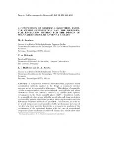
6.4 PANSHARPENING RESUTS FOR IKONOS DATA 6.4.1 Application at low resolution

The IKONOS multispectral and panchromatic images were resampled so that the pansharpened image is of the spatial resolution of 4m. The quality metrics were computed for the sharpened images and compared. The IKONOS images have a radiometric resolution of 11 bits per pixel compared to 8 bits per pixel for SPOT images. Also it is interesting to note the spectral overlap between the IKONOS panchromatic and multispectral images. The SPOT panchromatic image overlaps spectrally only with the first two bands of the SPOT multispectral image. This indicates that the IKONOS pan image has more corresponding information compared to the SPOT pan image. Figure 6.3 shows the original multispectral image with an area of interest (AOI). The AOI is chosen only to ease displaying the results. Sharpening was applied to the entire image. Figure 6.4 shows the multispectral, panchromatic, and sharpened results for the AOI.

- 54 The MSE and RMSE values were computed and are shown in Table 6.15. The values indicate that the pixel values are less distorted in the wavelet based method. The grey values of the Brovey and IHS sharpened images are heavily distorted. Table 6. 15 MSE and RMSE for IKONOS data: low resolution application

Method


RMSE 197.60 208.06 44.60 36.60

Band 2 MSE 46662.32 37964.39 6113.73 1907.64

RMSE 216.01 194.84 78.19 43.67

Band 3 MSE 20125.50 18554.11 8004.31 2357.97

Figure 6. 3 IKONOS multispectral image with area of interest (AOI)

RMSE 141.86 136.21 89.46 48.55

- 55 -

Figure 6. 4 Sharpening results for IKONOS data low resolution application a) IKONOS multispectral AOI, b) IKONOS panchromatic image AOI, c) IHS sharpened AOI, d) Brovey sharpened AOI, e) PCA sharpened AOI, f) Wavelet sharpened AOI

- 56 -

The spectral correlation between various spectral bands was computed for both the multispectral and sharpened images. The correlation with the panchromatic image was also computed. Table 6.16 shows the computed correlation values for the spectral bands. Table 6.17 shows the correlation values between the multispectral and panchromatic images. The correlation values indicate that the PCA-based sharpening and wavelet-based sharpening preserves the spectral information. The IHS and Brovey sharpened images have dominant pan information and in this particular case, the PCA sharpened image has a lower correlation, indicating very poor pan or spatial information. Table 6. 16 Correlation between spectral bands for IKONOS data: low resolution application


Band1&2 0.9749 0.9039 0.9418 0.9857 0.9422

Band 1&3 0.9499 0.9034 0.8158 0.9633 0.9002

Band 2&3 0.9806 0.9490 0.9535 0.9839 0.9805

Table 6. 17 Correlation between spectral bands and pan for IKONOS data: low resolution application


Band1&Pan 0.5952 0.6850 0.7984 0.3836 0.5689

Band 2&Pan 0.6936 0.7283 0.8075 0.4417 0.6786

Band 3&Pan 0.6952 0.7124 0.7340 0.4467 0.6876

The relative shift in the mean and the standard deviation of the histogram was computed for each of the sharpened bands. The values are shown in Tables 6.18 and 6.19. The values indicate that the mean of the Brovey and IHS sharpened have shifted towards the gray and the spread of the histograms has reduced for the Brovey sharpened bands.

- 57 Table 6. 18 Relative shift in the mean of spectral bands for IKONOS data: low resolution application


Band 1 (%) 63.57 67.46 7.78 -0.11

Band 2 (%) 65.23 56.87 15.48 -0.15

Band 3 (%) 53.07 43.13 24.23 -0.20

Table 6. 19 Standard deviation of spectral bands for IKONOS data: low resolution application


Band 1 52.5748 50.4385 33.3688 44.9617 46.6136

Band 2 84.6867 55.3898 34.3574 71.7861 68.9798

Band 3 96.2805 53.7983 26.6532 81.3750 77.2541

The NDVI values were computed for a vegetation subset from the multispectral, the wavelet sharpened, and PCA sharpened images. The correlation among the NDVI values was computed. The values are shown in Table 6.20. The NDVI values indicate that the NDVI feature for the wavelet-sharpened image is closer to the multispectral image compared to the PCA sharpened image. Table 6. 20 Correlation between NDVI values for MS and sharpened images for IKONOS data

Image Correlation PCA 0.7864 Wavelet 0.8762 The multispectral, wavelet sharpened, and PCA sharpened images were classified using an unsupervised K-means algorithm. The number of clusters or classes was set to ten. Each pixel was assigned a class label as a result of the classification. The percentage of pixels with a changed class label was computed. The values are shown in Table 6.21. The wavelet-sharpened image has a better class agreement with the multispectral image.

- 58 Table 6. 21 Comparison of classification for IKONOS data



6.4.2 Application at Full resolution

The IKONOS multispectral and panchromatic data at their original resolution of 4m and 1m were used to perform pansharpening. The sharpened image was compared to the original multispectral image. The multispectral image with an AOI and the multispectral panchromatic and wavelet sharpened image of the corresponding AOI are shown in Figures 6.5 and 6.6 respectively.

Figure 6. 5 IKONOS multispectral image with area of interest (AOI)

- 59 -

Figure 6. 6 Sharpening results for IKONOS data full resolution application a) IKONOS multispectral AOI, b) IKONOS panchromatic image AOI

- 60 -

Figure 6.6 Sharpening results for IKONOS data full resolution application (cont.) c) Wavelet sharpened AOI

The spectral error metrics were computed by resampling the multispectral to the appropriate resolution. The MSE and RMSE values are shown in Table 6.22.

Table 6. 22 MSE and RMSE for IKONOS data: full resolution application

Method


RMSE 209.73 206.29 36.96 36.09

Band 2 MSE 45672.59 36523.61 5790.8 1306.33

RMSE 213.71 191.11 76.09 36.14

Band 3 MSE 33824.55 17657.98 7193.81 1304.04

RMSE 183.91 132.88 84.81 36.11

The error values for the IHS and Brovey sharpened data are high compared to the PCA and wavelet sharpened data. The computed error metrics are reliable along

- 61 homogeneous areas but errors along other areas are not reliable as some of the new information in the sharpened image might be useful. The correlation between the different spectral bands and the correlation between spectral bands and panchromatic image were computed. The values are given in Tables 6.23 and 6.24. The wavelet-sharpened bands have spectral correlation similar to multispectral bands indicating preservation of spectral information. The correlation with the panchromatic band indicates more high frequency detail information in the sharpened image. The correlation values computed indicate that the IHS and Brovey sharpened bands have a good spatial information compared to the PCA and wavelet-sharpened bands. Also the wavelet-sharpened bands have a slightly higher correlation compared to PCA sharpened bands. Table 6. 23 Correlation between spectral bands for IKONOS data: full resolution application


Band1&2 0.9749 0.7028 0.9332 0.9291 0.9528

Band 1&3 0.9499 0.7838 0.7961 0.9552 0.9143

Band 2&3 0.9806 0.6096 0.9450 0.9624 0.9784

Table 6. 24 Correlation between spectral bands and pan for IKONOS data: full resolution application


Band1&Pan 0.5952 0.6580 0.8982 0.5056 0.6249

Band 2&Pan 0.6936 0.7085 0.9236 0.5868 0.6488

Band 3&Pan 0.6952 0.7354 0.8516 0.5862 0.6993

The relative shift in the mean and variation in standard deviation in the histogram of the sharpened bands were computed. The means of most of the Brovey and IHS

- 62 sharpened bands have shifted by at least 50%. The spread of the histogram is reduced for the Brovey sharpened bands. The histogram metrics are given in Tables 6.25 and 6.26. Table 6. 25 Relative shift in the mean of spectral bands for IKONOS data: full resolution application


Band 1 (%) 63.27 67.53 11.51 -0.36

Band 2 (%) 63.83 56.86 13.11 -0.41

Band 3 (%) 56.27 43.09 24.80 -0.64

Table 6. 26 Standard deviation of spectral bands for IKONOS data: full resolution application


Band 1 52.5748 54.0250 36.8661 54.8211 54.6182

Band 2 84.6867 58.5742 37.1149 88.2920 82.3292

Band 3 96.2805 54.6502 27.8347 100.734 92.5920

The entropy of each band of the multispectral and sharpened image was computed. The computed values are shown in Table 6.27. The values indicate an increase in entropy for all the sharpened images. The increase in information is more for the wavelet-sharpened bands compared to the other sharpened images. Table 6. 27 Entropy and Increase in information of spectral bands for IKONOS data

Method Original MS HIS Brovey PCA Wavelet

Band 1 6.2914 6.9864 6.9958 7.1454 7.3527

Increase 0.6950 0.7044 0.8540 1.0613

Band 2 6.4333 7.2587 7.1556 7.9076 7.9345

Increase 0.8254 0.7223 1.4743 1.5012

Band 3 6.3449 6.9947 6.7554 8.1652 8.0744

Increase 0.6498 0.4105 1.8203 1.7295

- 63 6.5 PANSHARPENING RESUTS FOR QUICKBIRD DATA 6.5.1 Application at low resolution

The QuickBird multispectral and panchromatic images were resampled so that the pansharpened image is of the spatial resolution of 2.8m. The original QuickBird multispectral image has a spatial resolution of 2.8m so this image provides ground truth for comparison with the sharpened images. The quality metrics were computed for the sharpened images and compared. Similar to IKONOS, the QuickBird images have a radiometric resolution of 11 bits per pixel. Figure 6.7 shows the original multispectral image with an area of interest (AOI). Sharpening was applied to the entire image. Figure 6.8 shows the multispectral, panchromatic, and sharpened results for the AOI. The error metrics MSE and RMSE values were computed and are shown in Table 6.28. The values indicate very less error in the pixel DN value for the wavelet-sharpened image. Table 6. 28 MSE and RMSE for QuickBird data: low resolution application

Method


RMSE 101.571 210.48 82.48 48.53

Band 2 MSE 10315.70 94953.08 19659.25 3163.77

RMSE 101.56 308.14 140.21 56.24

Band 3 MSE 10295.46 47314.10 14323.03 2969.85

RMSE 101.46 217.51 119.67 54.49

- 64 -

Figure 6. 7 QuickBird multispectral image with area of interest (AOI)

- 65 -

Figure 6. 8 Sharpening results for QuickBird data low resolution application a) QuickBird multispectral AOI, b) QuickBird panchromatic image AOI

- 66 -

Figure 6.8 Sharpening results for QuickBird data low resolution application (cont.) c) IHS sharpened AOI, d) Brovey sharpened AOI

- 67 -

Figure 6.8 Sharpening results for QuickBird data low resolution application (cont.) e) PCA sharpened AOI, f) Wavelet sharpened AOI

- 68 -

The spectral correlation values are shown in Table 6.29. The correlation between the spectral bands and the panchromatic image is shown in Table 6.30. Waveletsharpened bands have correlation similar to the multispectral bands. The subjective spatial quality of the wavelet-sharpened image is not as good as the PCA sharpened or the original multispectral image. The correlation values shown in Table 6.30 also indicate that the wavelet-sharpened bands have a lower correlation with the panchromatic image. The other techniques produced higher correlation with the panchromatic image and have a better spatial quality. Table 6. 29 Correlation between spectral bands for QuickBird data: low resolution application


Band1&2 0.9857 0.8681 0.9272 0.9818 0.9670

Band 1&3 0.9523 0.8729 0.8209 0.9201 0.9399

Band 2&3 0.9815 0.9663 0.9694 0.9701 0.9821

Table 6. 30 Correlation between spectral bands and pan for QuickBird data: low resolution application


Band1&Pan 0.7262 0.9334 0.8122 0.8167 0.7115

Band 2&Pan 0.7451 0.9832 0.8315 0.8352 0.7262

Band 3&Pan 0.7269 0.9824 0.7810 0.8175 0.7151

The relative shift in the mean and variations in standard deviation of the histogram of the spectral bands indicate that the histogram of the Brovey sharpened image has changed more compared to other images. The histogram of the PCA sharpened image has also been affected even though it had comparatively good spectral correlation and spatial quality. The values are shown in Tables 6.31 and 6.32.

- 69 Table 6. 31 Relative shift in the mean of spectral bands for QuickBird data: low resolution application


Band 1 (%) 3.90 71.19 8.67 -0.13

Band 2 (%) 2.71 67.64 10.16 -0.10

Band 3 (%) 4.23 64.42 13.49 -0.19

Table 6. 32 Standard deviation of spectral bands for QuickBird data: low resolution application


Band 1 108.87 92.96 38.84 77.10 103.68

Band 2 183.68 137.65 46.74 127.83 168.19

Band 3 157.35 117.14 29.76 107.91 142.62

The NDVI values were computed for a vegetation subset from the multispectral, wavelet sharpened, and PCA sharpened images. The correlation among the NDVI values was computed. The values are shown in Table 6.33. The NDVI values indicate that the NDVI feature for the wavelet-sharpened image is closer to the multispectral image compared to the PCA sharpened image. Table 6. 33 Correlation between NDVI values for MS and sharpened images for QuickBird Data

Image

Correlation

PCA

0.5909

Wavelet 0.8447

The multispectral, wavelet sharpened, and PCA sharpened images were classified using an unsupervised K-means algorithm. The number of clusters or classes was set to ten. Each pixel was assigned a class label as a result of the classification. The percentage of pixels with a changed class label was computed. The values are shown in Table 6.34.

- 70 The K-means classification algorithm resulted in a better class agreement with the wavelet-based method due to the preservation of spectral information in the wavelet sharpened image. Table 6. 34 Comparison of classification for QuickBird data



6.5.2 Application at Full resolution

The QuickBird multispectral and panchromatic data at their original resolution of 4m and 1m were used to perform pansharpening. The sharpened image was compared to the original multispectral image. The multispectral image with an AOI and the multispectral panchromatic and wavelet sharpened image of the corresponding AOI are shown in Figures 6.9 and 6.10 respectively. The error metrics were computed between the sharpened image bands and resampled multispectral bands. The MSE and RMSE values are shown in Table 6.35. The PCA and wavelet sharpened bands have very less pixel DN error compared to the resampled multispectral. Table 6. 35 MSE and RMSE for QuickBird data: full resolution application

Method


RMSE 225.81 210.10 74.35 24.62

Band 2 MSE 50926.57 94426.64 16225.31 606.37

RMSE 225.669 307.28 127.37 24.62

Band 3 MSE 48960.46 47106.04 11584.29 603.38

RMSE 221.27 217.03 107.63 24.56

- 71 -

Figure 6. 9 QuickBird multispectral image with area of interest (AOI)

- 72 -

Figure 6. 10 Sharpening results for QuickBird Data full resolution application a) QuickBird multispectral AOI, b) QuickBird panchromatic image AOI

- 73 -

Figure 6.10 Sharpening results for QuickBird data full resolution application c) Wavelet-sharpened AOI

The correlation between the different spectral bands and the correlation between spectral bands and panchromatic image were computed. The values are given in Tables 6.36 and 6.37. The wavelet-sharpened bands have spectral correlation similar to the multispectral bands indicating preservation of spectral information. The correlation values computed indicate that the PCA and Brovey sharpened bands have a good spatial information compared to the IHS and wavelet-sharpened bands.

- 74 Table 6. 36 Correlation between spectral bands for QuickBird data: full resolution application


Band1&2 0.9857 0.9693 0.9251 0.9761 0.9799

Band 1&3 0.9523 0.9481 0.8241 0.9210 0.9472

Band 2&3 0.9815 0.9627 0.9668 0.9692 0.9808

Table 6. 37 Correlation between spectral bands and pan for QuickBird data: full resolution application


Band1&Pan 0.7262 0.7325 0.8481 0.8430 0.8030

Band 2&Pan 0.7451 0.7435 0.8682 0.8591 0.8376

Band 3&Pan 0.7269 0.7099 0.8220 0.8362 0.8171

The relative shift in the mean and variation in standard deviation in the histogram of the sharpened bands were computed. The means of the Brovey and IHS sharpened bands have shifted by at least 60%. The spread of the histogram is also reduced for both the sharpened images. The histogram metrics are given in Tables 6.38 and 6.39. Table 6. 38 Relative shift in the mean of spectral bands for QuickBird data: full resolution application


Band 1 (%) 75.72 71.22 10.07 0.06

Band 2 (%) Band 3 (%) 82.97 69.87 67.62 64.44 11.90 15.78 0.05 0.07

- 75 Table 6. 39 Standard deviation of spectral bands for QuickBird data: full resolution application


Band 1 108.87 46.28 41.94 84.27 107.60

Band 2 183.68 46.86 50.63 142.14 181.01

Band 3 157.35 46.36 31.68 121.66 154.74

The entropy of each band of the multispectral and sharpened image was computed. The computed values are shown in Table 6.39. The values indicate a decrease in entropy for the Brovey and IHS sharpened images. The increase in information is more for the wavelet-sharpened bands compared to the PCA technique. Table 6. 40 Entropy and Increase in information of spectral bands for QuickBird data


Band 1 7.5506 7.0745 6.8340 7.6740 7.9214

Increase -0.4761 -0.7166 0.1234 0.3708

Band 2 8.5567 7.1138 7.1397 8.5466 8.7054

Increase -1.4429 -1.4170 -0.0101 0.1487

Band 3 8.3619 7.1231 6.4840 8.3826 8.5575

Increase -1.2388 -1.8779 0.0207 0.1956

CHAPTER VII CONCLUSIONS In this study, quantitative image quality metrics for pansharpened images are presented. The MSE and RMSE, correlation coefficients between the spectral bands, correlation coefficients between the spectral bands and the panchromatic image, relative shift in the mean and variations in standard deviation in the histogram of the image bands, correlation between NDVI values for the multispectral and sharpened images, increase in information for the sharpened bands, and changes in classification are the quantitative metrics used in this study. The pansharpening algorithms were tested using three different sets of satellite data viz., SPOT, IKONOS, and QuickBird Data. The multispectral and panchromatic image had different spatial resolutions and spectral ranges. The sharpening algorithms were applied to images both a low resolution and at full resolution. The wavelet based sharpening consistently produced sharpening results with better spectral quality compared to other techniques studied. The spatial quality of the wavelet-sharpened image varied between the data sets. In the wavelet-based method, the spatial detail information is derived from the panchromatic image and added to the spectral information. For other techniques, such as IHS and PCA, the spectral information is derived form the multispectral image and added to the panchromatic image. The spatial performance of the wavelet sharpening is heavily dependent on a

- 76 -

-77number of factors. They are •

High co-registration accuracy between the multispectral and panchromatic image in the order less than half a pixel.

•

The resampling technique used in the production of the multispectral and panchromatic image Ability of the mother wavelet and DWT to consistently derive more quality high frequency spatial information from the panchromatic images, which are of different spatial resolution. In the PCA and IHS sharpening, the panchromatic image replaces the PC1 or

intensity component. The difference in the gray values between the panchromatic image and PC1 or intensity bands affects the spectral quality of the sharpened image. The Brovey sharpening uses a ratio technique and hence the sharpened image has good contrast but due to this normalization, the DN values are changed a lot and the histogram of the image bands are affected. The wavelet-sharpened images have a very good spectral quality. The spatial quality of the sharpened images varies based on the data used for sharpening. Hence there is a need to investigate with different combination models in the wavelet domain to make the wavelet-based sharpening more robust spatial quality.

REFERENCES [1]

C.Pohl, J.L. Van Genderen, “Multisensor image fusion in remote sensing: concepts, methods and application”, International Journal of Remote Sensing, vol. 99, no. 5, pp. 823-854,1998.

[2]

L. Wald, “ Some terms of reference in data fusion”, IEEE Transactions on Geoscience and Remote Sensing, vol. 37, no. 3, pp. 1190-1193, May 1999.

[3]

W. J. Carper, T. M. Lillesand, R. W. Kiefer, “The use of intensity-huesaturation transformations for merging SPOT panchromatic and multispectral image data”, Photogrammetric Engineering and Remote Sensing, vol. 56, no. 4, pp. 459-467, April 1990.

[4]

P. Chavez, Jr., S. Sides, J. Anderson, “Comparison of three different methods to merge multiresolution and multispectral data: Landsat TM and SPOT panchromatic”, Photogrammetric Engineering and Remote Sensing, vol. 57, no. 3, pp. 295-303, March 1991.

[5]

Y.Zhang, “A new merging method and its spectral and spatial effects”, International Journal of Remote Sensing, vol. 20, no. 10, pp. 2003-2014.

[6]

J. Nunez, X. Otazu, O. Fors, A. Prades, V. Pala, R. Arbiol, “ MultiresolutionBased Image fusion with additive wavelet decomposition”, IEEE Transactions on Geoscience and Remote Sensing, vol. 37, No. 3,pp. 12041211, May 1999.

[7]

R. King, J. Wang, “ A wavelet based algorithm for pansharpening Landsat 7 imagery”, Proceedings of the International Geoscience and Remote Sensing symposium, vol. 2, pp. 849-851, 2001.

[8]

A. Fanelli, A. Leo, M. Ferri, “Remote sensing images data fusion: a wavelet transform approach for urban analysis”, Proceedings of the IEEE/ISPRS joint workshop on remote sensing and data fusion over urban areas, pp. 112-116, 2001.

[9]

Shutao Li, James T. Kwok, Yaonan Wang, “Using the discrete wavelet frame transform to merge Landsat TM and SPOT panchromatic images”, Information Fusion, vol.3, pp. 17–23, 2002.

[10]

T. Ranchin, B. Aiazzi, L. Alparone, S. Baronti, L. Wald, “Image fusion—the ARSIS concept and some successful implementation schemes”, ISPRS Journal of Photogrammetry & Remote Sensing, vol. 58, pp 4-18, 2003. - 78 -

- 79 -

[11]

L. Chipman, T. Orr, L. Graham, “ Wavelets and image fusion”, Proceedings of the International Conference on Image Processing, vol.3, pp 23-26, 1995.

[12]

Din-Chang Tseng, Yi-Ling Chen, and Michael S.C. Liu, “Wavelet-based multispectral image fusion”, Proceedings of the International Geoscience and Remote Sensing Symposium, vol. 4, pp. 1956-1958, 2001.

[13]

N. Ouarab, M. Achir, N. Khettal, Y. Smara, “Spatial enhancement of satellite images using data fusion algorithms in the wavelet domain”, Proceedings of the IEEE/ISPRS joint workshop on remote sensing and data fusion over urban areas, pp.293 – 298, 2001.

[14]

R. Gonzalez, R. Woods, Digital Image Processing, 2nd edition, Prentice Hall, Upper Saddle River, NewJersey, 2002.

[15]

A.R. Smith, “Color gamut transform pairs”, Computer graphics, vol.13, no.3, pp.12-19, 1978.

[16]

E.M. Schetselaar, “Fusion by the IHS transform: should we use cylindrical or spherical coordinates?”, International Journal of Remote Sensing, vol. 19, no. 4, 759-765.

[17]

K. Castleman, Digital Image Processing, Prentice Hall, Upper Saddle River, NewJersey, 1995.

[18]

C. Burrus, R. Gopinath, H. Guo, Introduction to wavelets and wavelet transforms a primer, Prentice Hall, Upper Saddle River, NewJersey, 1998.

[19]

D. Hall, J. Llinas, Handbook of multisensor data fusion, CRC Press, 2001.

[20]

ENVI User’s guide, ENVI version 3.6, 2nd edition, 2002.

[21]

M. Unser, T. Blu, “Mathematical properties of the JPEG2000 wavelet filters”, IEEE Transactions on Image Processing, vol. 12, no. 9, pp.1080 – 1090, September 2003.

[22]

A. Jain, Fundamentals of Digital Image Processing, 1st edition, Prentice Hall, Prentice Hall, Upper Saddle River, NewJersey, 1988.

[23]

L. Wald, T. Ranchin, M. Mangolini, “Fusion of satellite images of different spatial resolutions: accessing the quality of resulting images”, Photogrammetric engineering and remote sensing, vol. 63, no. 6, pp. 691-699, June 1997.

[24]

V. Vijayaraj, N.H. Younan, C.G. O’Hara, “ Quality metrics for multispectral image processing”, Proceedings of the ASPRS Annual Conference, Denver, May 2004.

[25]

A. Eskicioglu, P. fisher, “ Image quality measures and their performance”, IEEE Transactions on Communications, vol. 43, no.12, pp. 2959-2965, December 1995.

[26]

I. Parcharidis, M. Kazi-Tani, “Landsat TM and ERS data fusion: a statistical approach evaluation for four different methods”, Proceedings of the

- 80 International Geoscience and Remote Sensing Symposium, vol. 5, pp. 2120 – 2122, 2000. [27]

R. Duda, P. Hart, D. Stork, Pattern Classification, 2nd edition, John Wiley & Sons, 2001.

[28]

F. Van Der Meer, “ What does multisensor image fusion add in terms of information content for visual interpretation?”, International Journal of Remote Sensing, vol. 18, no. 2, pp. 445-452. 1997.

quantitative comparison of pansharpening algorithms - CiteSeerX

quantitative comparison of pansharpening algorithms - CiteSeerX

Suggest Documents

quantitative comparison of pansharpening algorithms - CiteSeerX

New Sparsity Based Pansharpening Algorithms for

Quantitative comparison of languages - CiteSeerX

the effect of pansharpening algorithms on the resulting orthoimagery

a comprehensive review of pansharpening algorithms ... - ISPRS Annals

quantitative modelling and comparison of communication ... - CiteSeerX

iTRAQ Quantitative Proteomic Comparison of Metastatic ... - CiteSeerX

Comparison of WiMAX scheduling algorithms and ... - CiteSeerX

comparison of density-based clustering algorithms - CiteSeerX

a comparison of genetic algorithms, parti - CiteSeerX

Comparison of Blind Source Separation Algorithms - CiteSeerX

Comparison of Probabilistic Optimization Algorithms for ... - CiteSeerX

comparison of density-based clustering algorithms - CiteSeerX

Quantitative Evaluation of Distributed Algorithms

Comparison-based algorithms: worst-case optimality ... - CiteSeerX

Comparison Methodology for Ray Shooting Algorithms - CiteSeerX

Pansharpening With Matting Model

QUANTITATIVE COMPARISON OF BOTTLENOSE DOLPHIN ...

Comparison of neural classification algorithms

Comparison of Metaheuristic Algorithms through

Comparison of quantitative myocardial perfusion

Quantitative biomechanical comparison of ankle

Comparison of Decentralized Tracking Algorithms

Comparison of assembly algorithms for improving rate of ... - CiteSeerX