learning curves in process simulation models improves the accuracy and .... programming and software tool experience of the project team developing the ...
Quantitative Control of Process Changes Through Modeling, Simulation and Benchmarking Nancy Eickelmann, Animesh Anant, Sang Hyun, Jongmoon Baik SSERL, Motorola, 1303 E. Algonquin Rd. Schaumburg, IL, 60196, USA +1-847-576-4040
ABSTRACT - This paper provides a comparison of two learning curve models that are used to quantify the productivity increase experienced as a result of process improvements and new technology adoption. Evaluating productivity increase is essential for estimating the cycle time and effortrequired to complete a software project. At SSERL, we have been using software process modeling and simulation to predict the impact of process and technological changes. Incorporating productivity learning curves in process simulation models improves the accuracy and validity of these models.
KEY WORDS
- Process Model, Simulation, Learning Curve, COCOMO I1
1. INTRODUCTION Software process modeling and simulation is a wellproven technology that has been used by the software engineering community since the late 1980s to support prediction, control and understanding of the software development process. Process simulation models have also been used to evaluate process improvement, technology insertion and defect prevention activities. Process improvement and technology insertion activities require that the current process or tools be changed. The productivity gains from process improvement and technology insertion activities are not immediate but occur over time. As the software development team gets familiar with the new process and technology, the productivity increases. The total gain and the rate of increase in productivity are significant factors in estimating the required effort and schedule for a particular software project. Productivity learning curves can be used to model the increase in productivity. We can use the COCOMO I1 cost drivers [4] or other learning curve models such as the one described in [5] to model productivity increase. In this paper, we have evaluated the productivity learning curve as defined in [5] for use with process modeling and simulation technology and compared it with the COCOMO I1 model cost drivers.
Section 2 provides an overview of the process modeling and simulation technology and definitions to set a common ground for discussion. Section 3 is divided into two sub-sections and introduces the productivity learning curve model and the COCOMO I1 model. Section 4 presents the comparison between the productivity learning curve and the COCOMO I1 model and in Section 6, we discuss the conclusions and lessons learned.
2. OVERVIEW OF PROCESS MODELING AND SIMULATION Process modeling and simulation facilitates the understanding of the "As-Is" process, and supports prediction of the impacts of process changes and technology insertions on schedule, quality, cycle time and effort for the software productivity improvement (SPI) activities. Software process modeling and simulation is being applied across the lifecycle in the software engineering domain, to provide irrdepth analysis in requirements management, project management, training and process improvement activities. Simulation can be used to improve software development processes at all levels of SEI-CMM, however it is particularly appropriate at higher maturity levels (level 3, 4, & 5), because it requires metrics and well-defined process behaviors. It is also useful for organizations at the initial and defined CMM levels by characterizing the current process and documenting subprocess areas that would benefit the most from process improvement efforts. Software process simulation modeling can be used for the following: - Strategic Management: simulation can help address a broad range of strategic management issues. Should the work be distributed across sites or should it be centralized at one location? Would it be better to perform the work in-house or to out-source (subcontract) it?
Planning: simulation can support management planning such as effort, cost, schedule and product quality prediction, forecasting staffing levels etc. Control and Operational Management: simulation can support project tracking and oversight because key project parameters (such as, actual status and progress on the work products, resource etc.) can be monitored and compared against planned values computed by the simulation. Process Improvement and Technology Adoption: simulation can aid specific process improvement and technology adoption decisions by forecasting the impact of a potential change before putting it into actual practice in the organization. At the Software and System Engineering Research Lab (SSERL), we have used this technology to predict the impact of process changes and technology insertions on schedule, quality, and effort, and to provide insight into optimal strategies to achieve Six-Sigma? goals. The inputs to the model are product characteristics such as the size, number of features, complexity, etc. and process characteristics such as experience, percentage of reuse, etc. The actual model is based on the current process and captures the relationships between the various factors affecting the software development process. Different scenarios can then be developed to predict the impact of the process changes and technology insertion activities. The outputs of the m d e l are usually cycle time, effort and/or quality. The model is then validated conceptually as well as quantitatively. Conceptual validation is usually done through discussions with the project managers and subject matter experts. Quantitative validation is done by comparing the model outputs with the actual outputs. Figure 1 shows our six-step approach to modeling a software process.
Step 1. Planning Analyze a defined process, define the model scope, and determine key parameters. Step 2. Data Collection & Analysis: Gather data and determine the statistical significance of parameters. Step 3. Build Baseline Simulation model: Develop baseline "As-Is" simulation model based on gathered data and analysis results. Step 4. Validation of the Model: Validate the model if the model outputs are meaningful. Step 5. What-If Analysis: Create scenarios for future process changes or new technology insertions in the process, experiment the model with them, and analyze the impacts of those changes into the system process. Step 6. Collect more data & Refine the Model: Gather more data to refine the simulation model. We also provide a set of definitions that will provide a consistent context of understanding for the reader. Some of the terms are defined by their original context
specifically those terms used in the COCOMO I1 model. The PLC or productivity learning curve was developed in Motorola Labs and is defined for the reader.
Planning
Analysis
r - -
I I
I--
Simulation Model
I
L-,
Model
I$] Experiment wl Scenarios Analysis of Results #-
FI
Collect more data & Refine the Model
Figure 1. Stepwise Simulation Modeling Approach COCOMO I1 - Constructive Cost Model (COCOMO) is a model that allows one to estimate the cost, effort and schedule when planning a new software development activity. The COCOMO I1 model is an update to the original COCOMO 81 model.
APEX - Applications Experience (APEX) cost driver. The rating for this cost driver depends on the level of applications experience of the project team developing the software system or subsystem.
LTEX - Language and Tool Experience (LTEX) cost driver. The rating for this cost driver depends on the level of programming and software tool experience of the project team developing the software system or subsystem.
PLEX - Platform Experience (PLEX) cost driver. The rating for this cost driver depends on the platform experience of the project team developing the software system or subsystem.
Model - A model is an abstraction or simplified representation of a real or conceptual complex system. A model is designed to
display significant features and characteristics of the system that one wishes to study, predict, modify or control.
$100.00and the cost for the second unit is $70.00,then the "learning curve" is 70%.
Simulation Model - A simulation model is a computerized model that possesses the characteristics described above and that represents some dynamic system or phenomenon. Simulations are generally employed when the complexity of the system being modeled is beyond what static models can usefully represent.
In software development, product volume is not a good measure because creations are unique. Further, when a creation is duplicated the cost of duplication is extremely small in proportion to the engineering cost. Therefore, we need measures other than production cost to evaluate learning curves for software development. We may use any of the following three measures [5]: 1. Faults sourced per KAELOC to (faults created by) a process step. 2. Percent faults remaini ng per KAELOC within a process step. 3. Productivity per KAELOC within a process step attributed to a change.
Software Process Simulation Model - A software process simulation model focuses on a particular software development~maintenance/evolutionprocess. It can represent a process as currently implemented (as-is), or as planned for future implementation (to-be). Productivity - In its broadest form. productivity may be described as a measure of how well the resources in a firm are brought together and used to accomplish a set of results. At Motorola. the following definition for productivity is used: Productivity =
Total Size of Product (in KAELOC) Total Effort (in Staff -Months)
(1)
KAELOC - Kilo Assembly Equivalent Lines of Code Learning Curve - The learning curve was adapted from the historical observation that individuals who perform repetitive tasks exhibit an improvement in performance as the task is repeated a number of times. The learning curve may be defined as the ratio of the manufacturing cost at the manufacture of unit N to the manufacturing cost at unit N-1.
In the next section, we have outlined two different approaches to modeling productivity learning curves.
4. MODELING PRODUCTIVITY GROWTH As stated earlier, measuring the increase in productivity resulting from process and technological changes is crucial in estimating the effort and schedule required to complete a software project. There are several productivity learning curve models, however, these models are generally used for manufacturing processes and are not applied to the software development process. In the next two sub-sections, we discuss two learning curve models that can be applied to the software development process.
4.1 Productivity Learning Curve The software learning curve model [5]is conceptually based on the learning curve used to quantify improvement in manufacturing cost. The learning curve is the ratio of the manufacturing cost at the manufacture of unit N to the manufacturing cost at unit N1. For instance, if the cost to manufacture the first unit is
The faults sourced learning curve for the process is defined as the faults created per KAELOC by the process in year N divided by the faults created by the process per KAELOC in year N-1. The productiGty learning curve for the process is defined as the number of staffmonths of effort per KAELOC in year N divided by the staff-months of effort per KAELOC in year N1.For example, if in year N-1 we created 100 faults in a project using 100 staff-days and in year N we created 90 faults in an equivalent project with the project taking 70 staffdays, then we have a 90% lesrning curve for in-process faults sourced and a 70% learning curve for productivity. A smaller learning rate represents faster learning, i.e., a 60% learning curve represents faster learning than a 70% learning curve. The in-process faults remaining learning curve is the ratio of the percentage of in-process faults remaining per KAELOC upon exiting a lifecycle phase in the current year. divided by the percentage of in-process faults per KAELOC remaining in the same phase in the previous year. That is, if in year N-1,there are 5 defects entering the coding phase and 5 defects created in the coding phase and only 6 of the defects are detected, then 40% of the faults remain. If in year N, there are 4 defects on entry, 4 more defects are created in the phase and only 5 defects are detected, then 37.5% of the faults remain. In this case, the in-process faults remaining learning curve is (37.5%/40%) * 100 or
93.75%. Table 1 shows the learning curve values needed for a 10X improvement in productivity in 5 years. Achieving sustained 55% productivity curves is very difficult while making pocess and technological changes. We have to be able to forecast the impact of these changes through pilot projects, which are expensive, or through modeling and simulation.
Table 1. Learning Curve for 10X in 5 Years (from [51) Effort Improvement Start Dec-97 Dec-98 Dec-99 Dec-00 Dec-01 Req Spec 10.00 5.50 3.03 1.66 0.92 Req Model Phase 10.00 5.50 3.03 1.66 0.92 High Level Design 5.00 2.75 1.51 0.83 0.46 Detailed Design 15.00 8.25 4.54 2.50 1.37 Code Phase 30.00 16.50 9.08 4.99 2.75 Unit test 10.00 5.50 3.03 1.66 0.92 Integration Test 10.00 5.50 3.03 1.66 0.92 System Test 10.00 5.50 3.03 1.66 0.92 Total Effort 100.00 55.00 30.25 16.64 9.15 Improvement Ratio 1.8 3.3 6.0 10.9 Target Ratio 10 Productivity Learning Curve Req Spec 55% 55% 55% 55% 55% 55% 55% 55% Req Model Phase High Level Design 55% 55% 55% 55% 55% 55% 55% Detailed Design 55% Code Phase 55% 55% 55% 55% Unit test 55% 55% 55% 55% Integration Test 55% 55% 55% 55% Svstem Test 55% 55% 55% 55%
In section 4.2, vce discuss the COCOMO I1 model that can also be used to derive a productivity learning curve model.
4.2 COCOMO I1 Model COCOMO I1 is a model that allows one to estimate the cost, effort, and schedule when planning a new software development activity [41. It has two main sub-models, Early Design and Post Architecture. The Early Design model is a high-level model that is used to explore architectural alternatives or incremental developmental strategies. The Post Architecture model is a detailed model that is used once the project is ready to develop and sustain a fielded system. Both the Post-Architecture and Early Design models use the same approach to estimate the amount of effort and schedule required to complete a software project. The amount of effort in person-months. PM, is estimated by the formula: n
P M = A * s ~ z ~ ~ * ~ E M , (2) i=1
where A = 2.94 As can be seen from the above equation, the inputs for estimating effort are size; a constant, A; an exponent E; and a number of values called effort multipl iers (EM). The constant A is obtained by calibration to the actual parameters and effort values for the 161 projects studied while developing the COCOMO I1 model. The size is
estimated in Kilo Source Lines of Code (KSLOC) and can also be estimated from unadjusted function points. The exponent E is an aggregation of five scale factors that account for the relative economies and diseconomies of scale encountered for software projects of different sizes. Each scale factor has a range of rating levels, from Very Low to Extra High and each rating level is assigned a weight. For example, all the scale factors with an Extra High rating are assigned a weight of 0. The exponent E is then determined using equation 3. 5
E = B + o . o ~ s5 * ~
(3)
j= 1
where B = 0.91 The constant B is calibrated from the 161 projects used to develop the model. Cost drivers are used to capture various characteristics of software development that impact the total effort required to complete a project. All COCOMO I1 cost drivers have qualitative rating levels ranging from Extra Low to Extra High. Each of these rating levels has a value called an effort multiplier (EM) associated with it. For example, the effort multiplier for the Nominal rating is 1.0. If a cost driver's rating level causes more software development effort, then its corresponding level is above 1.0. Conversely. if the cost driver's rating level reduces the effort, then the corresponding EM is less than 1.0. The number of effort multipliers is 17 for the Post Architecture model and 7 for the Early Design model. In this paper, we have compared only the PostArchitecture cost drivers with the Productivity Learning Curve. Three of the seventeen cost drivers can be used to estimate the impact of experience and learning on effort. These three cost drivers are APEX. LTEX and PLEX. The ratings for the Applications Experience (APEX) cost driver are dependent on the project team's experience with the type of application being developed. The ratings for the Language and Tool Experience (LTEX) depend on the programming language and software tool experience of the development team. The ratings for the Platform Experience (PLEX) driver depend on the platform experience, database, networking etc. capabilities of the development team. A very low rating for these cost drivers is for experience of less than two months, while a very high rating is for application experience of six years or more. For example, for the LTEX multiplier, if the experience increases from a Very Low rating to a Very Hgh rating, a 43% increase in productivity is obtained. The ratings for the cost drivers are shown in table 2.
at 80%, 70% and 55%. Linear interpolation is tsed to arrive at the intermediate values for the combined multiplier, e.g., the value of the combined multiplier at 2 years is 0.865. Therefore, the effort required to complete the project with 2 years experience is 86.5 staff-months.
Table 2. COCOMO I1 multipliers
Rating Levels
APEX LTEX PLEX Combined Multiplier
1.20 1.19 1.74
Table 3. Staff-months required (Calculated using COCOMO 11 and PLC multipliers) 1.31
1.00
0.73
0.68
Table 1 also shows the ratings for a Combined Multiplier that we have defined. The Combined Multiplier is derived from the following equation: Combined Multiplier = APEX * LTEX * PLEX
( 0 1 1 1 2 1 3 1 4 1 5 1 6
Year
I
In the next section, we have presented the comparison between the productivity learning curve and the combined multiplier derived from COCOMO I1 cost drivers.
5. COMPARISON We have compared the Combined Multiplier with three Productivity Learning Curves (PLCs), an 80% learning curve, a 70% learning curve and a 55% learning curve. Since, the very high rating level for the COCOMO multiplier is for experience of 6 years or more, we have compared the COCOMO multiplier and the PLC over a period of 6 years. The assumptions made in this comparison analysis are listed below:
1) At Motorola, effort is measured in staff-months while in COCOMO I1 effort is expressed in person-months. For this analysis, we have assumed that staff-months and person-months are equivalent.
1 174 1 100 1
PLC at 70% PLC at 55%
(4)
We have used the Combined Multiplier to obtain a single learning curve model when the three cost drivers; APEX, LTEX and PLEX are significant factors in the software development effort.
based PLC
174 174
122 96
86
1
60 29
85 53
68
1
42 16
63 29 9
1
58
1
20 5
Table 3 shows that the productivity improvement in the first year is very high for the COCOMO I1 combined multiplier. This productivity improvement is close to the productivity improvement obtained by being on a 55% leaming curve. After the first year, the productivity does not increase as rapidly for the COCOMO I1 multiplier. In fact, the effort required by an organization on a 70% leaming curve after 2 years is less than the effort required by an organization following the COCOMO I1 curve. At the end of 6 years. an organization on a 55% learning curve would take only 5 staff-months to complete the project while an organization following the COCOMO I1 curve would take 58 staff-months. Therefore, the productivity improvement resulting from the COCOMO I1 multiplier is very gradual, especially in the 3-6 years time period. Figure 2 is the graphical representation for table 2. As can be seen from the graph, for the first year, the COCOMO 11 learning curve and the 55% productivity learning curve are similar. However, at the end of 6 vears. even the 80% learning curve falls below the COCOMO I1 curve. L,
I
PLC Comparison Analysis
tCOCOMO II based PLC
2) To simplify the calculation, we have assumed that the initial staff-months required for the project was 174 staff-months. We have chosen this initial value as the very low rating level for the COCOMO combined multiplier is 1.74. The staff-months required for the project at year 0 is 174 staff-months. Table 3 shows the staff-months required to complete the project in successive years using the COCOMO I1 combined multiplier and the productivity learning curves
1
73
+PLC at 80%
0
1
2
3 4 Years
5
6
7
-t-
PLC at 70%
-
PLC a! 55%
Figure 2. Productivity Comparison Analysis The salient differences between the productivity learning curve (PLC) and the learning curve derived from the COCOMO I1 cost drivers are: The COCOMO I1 multipliers are static while the PLC can change from year to year. The COCOMO I1 model has separate multipliers for the Early Design phase and the PostArchitecture phases. Even though in this paper, we have considered only the Post-Architecture multipliers, we can use the PREX (Personnel Experience) Early Design cost driver for comparison and analysis as well. The PLC model, however, can be used to derive productivity learning curves for the phase-level as well as the element-level. For example, using the PLC model we can define learning curves for a phase such as the coding phase or a phase element such as code inspections, code reviews, etc. Therefore the scope of the PLC multiplier is greater than that of the COCOMO I1 combined multiplier. All the cost drivers in the COCOMO I1 model impact effort and therefore, productivity. However, only APEX, LTEX and PLEX are time-dependent. The other cost drivers are not time-dependent and cannot be used in this analysis. The above analysis shows that the COCOMO I1 cost drivers should be used when the rate of leaming is much faster initially. COCOMO I1 drivers can also be used when there is no prior data to judge the productivity learning curve for an organization. Since, COCOMO I1 driver values are based on a Bayesian calibration of data collected from 161 industry-wide projects and expert opinion, they are a good starting point for modeling productivity increase. Productivity learning curves are very useful when modeling a part of the software development process, such as the testing process or the inspection process, etc. In this case, phaselevel productivity leaming curves can be used. Productivity learning curves should also be used when the learning rate changes from year to year. For example, an organization may be on a 70% learning curve in the first year and a 55% learning curve in the second year.
6. CONCLUSION In this paper, we have analyzed the productivity learning curves (PLCs) and compared the results with a simulation process model that used the COCOMO I1 cost drivers as input values of key productivity variables. The PLC was evaluated at 80%, 70% and 55% productivity gains (see Table 3) and the COCOMO I1 cost drivers of APEX, LTEX, PLEX were computed for five ordinal scale values from very low to very high. The
simulation model provided productivity estimates from 2 months to 6 years. The productivity learning curve was applicable only on a year-to-year comparison. Advantages of using the PLC include benchmarking from year to year, evaluating longer-term trends and cumulative effects of training and insertion of new technologies. The advantages of the simulation model using the COCOMO I1 cost drivers is short-term impacts in productivity including productivity loss or gain, and interactions among key factors that provide insight into what aspect of the process is most sensitive to changes and those aspects most likely to result in positive results when changed.
7. REFERENCES [ 11 Abdel-Hamid, Tarek, Madnick, Stuart E., "Software Project Dynamics", Prentice Hall. 199 1.
[2] Anant, Animesh, "An Approach to the SemiAutomatic Generation of Software Functional Architectures", Masters Thesis, University of Maryland, 2000. [3] Baik. Jongmoon, Eickelmann, Nancy, Abts. Chris. "Empirical Software Simulation for COTS Glue Code Development and Integration." In the Proceedings of the 2 5th~ n n u a COMPSAC, l October 8- 12, 200 1. [4] Boehm, B.. et. al., "Software Cost Estimation with COCOMO 11",Prentice Hall, 2000. [5] Dorenbos, David. "A Learning Curve Model for the Quality and Productivity of the Software Development Process", Motorola Software Engineering Symposium 1993. [6] Eickelmann, Nancy S., "Empirical Studies to Identify Defect Prevention Opportunities LGing Process Simulation Technologies" NASA Software Engineering Workshop, November 27-29, 200 1. [7] Eickelmann. Nancy S., "Analyzing Defect Opportunities in the Software Lifecycle with Process Simulation Technologies," In the Proceedings of the 71h International Conference on Information Systems Analysis and Synthesis, Orlando, FL., July 22-25, 2001. [8] Eickelmann, Nancy S., "Applying Simulation Technologies to Manage Test Practices," In the Proceedings of the lgth International Conference on Testing Computer Software, June 18-22, 200 1 , [9] Eickelmann, Nancy S., "Defining Meaningful Measures of IT Productivity with the Balanced
Scorecard" In the Proceedings of the Information Resource Management Conference IRMA 2001, May 20-23, 2001. 1101 Hanakawa, Noriko, Morisaki, Syuji, Matusmoto, Ken-ichi, "A Learning Curve Based Simulation Model for Software Development", In the Proceedings of the 1998 International Conference on Software Engineering, 1998. [ l l ] Humphrey, W. S., Kellner, M. I., "Software Process Modeling: Principles of Entity Process Models", Technical Report, CMUISEI-89-TR-2, Software Engineering Institute, Camegie Mellon University, Pittsburgh, Pennsylvania, 1989. 1121 Kellner, M. I., Madachy, R. J., Raffo, D. M., "Software Process Simulation Modeling: Why? What? How?", Journal of Systems and Software, Vol. 46. No. 213, 1999. [13] Law, A. M., Kelton, W. D., "Simulation Modeling and Analysis", McGraw-Hill, Inc. New York, 1991. [14] Raccoon, L. B. S., "A Learning Curve Primer for Software Engineers", In Software Engineering Notes, Volume 2 1, Number 1, January 1996, ACM Press.