arXiv:0710.3043v2 [quant-ph] 5 Aug 2008
Quantum central limit theorem for continuous-time quantum walks on odd graphs in quantum probability theory S. Salimia a
∗
Department of Physics, University of Kurdistan, Kurdistan 51664, Iran.
August 5, 2008
∗
E-mail:
[email protected]
1
2
continuous-time Quantum walk Abstract The method of the quantum probability theory only requires simple structural data of graph and allows us to avoid a heavy combinational argument often necessary to obtain full description of spectrum of the adjacency matrix. In the present paper, by using the idea of calculation of the probability amplitudes for continuous-time quantum walk in terms of the quantum probability theory, we investigate quantum central limit theorem for continuous-time quantum walks on odd graphs. Keywords: Continuous-time quantum walk, Spectral distribution, Odd graph. PACs Index: 03.65.Ud
continuous-time Quantum walk
1
3
Introduction
Two types of quantum walks, discrete and continuous time, were introduced as the quantum mechanical extension of the corresponding random walks and have been extensively studied over the last few years [1, 2]. Random walks on graphs are the basis of a number of classical algorithms. Examples include 2-SAT (satisfiability for certain types of Boolean formulas), graph connectivity, and finding satisfying assignments for Boolean formulas. It is this success of random walks that motivated the study of their quantum analogs in order to explore whether they might extend the set of quantum algorithms. Several systems have been proposed as candidates to implement quantum random walks. These proposals include atoms trapped in optical lattices [3], cavity quantum electrodynamics (CQED) [4] and nuclear magnetic resonance (NMR) in solid substrates [5, 6]. In liquid-state NMR systems [7], timeresolved observations of spin waves has been done [8]. It has also been pointed out that a quantum walk can be simulated using classical waves instead of matter waves [9, 10]. A study of quantum walks on simple graph is well known in physics(see [11]). Recent studies of quantum walks on more general graphs were described in [12, 13, 14, 15, 16, 17, 18]. Some of these works studies the problem in the important context of algorithmic problems on graphs and suggests that quantum walks is a promising algorithmic technique for designing future quantum algorithms. There is one approach for investigation of continuous-time quantum walk (CTQW) on graphs using the spectral distribution associated with the adjacency matrix of graphs [19, 20, 21, 22, 23]. Authors in Ref.[19] have introduced a new method for calculating the probability amplitudes of quantum walk based on spectral distribution which allows us to avoid a heavy combinational argument often necessary to obtain full description of spectrum of the Hamiltonian. It is interesting to investigate the CTQW on graph when the graph grows as time goes
4
continuous-time Quantum walk
by. In order to study a quantum system in full detail, its Hamiltonian needs to be diagonalized. With increasing dimension of the Hilbert space, the diagonalization of an operator becomes a very tedious task. In fact, we discuss this question in the CTQW as a quantum central limit theorem for CTQW. In this paper we try to investigate quantum central limit theorem for CTQW on growing odd graph via spectral distribution. The organization of the paper is as follows. In section 2, we give a brief outline of graphs and introduce odd graph. In Section 3, we review the stratification and quantum decomposition for adjacency matrix of graphs. Section 4 is devoted to the method of computing the amplitude for CTQW, through spectral distribution µ of the adjacency matrix. In the first subsection of section 5 we evaluate the CTQW on finite odd graph and the in second subsection 5, we investigate quantum central limit theorem for CTQW on odd graph. The paper is ended with a brief conclusion and one appendix which contains determination of spectral distribution by continued fractions method.
2
Odd graph
In beginning we present a summery of graph and then we introduce odd graph. A graph is a pair G = (V, E), where V is a non-empty set and E is a subset of {{α, β}|α, β ∈ V, α 6= β}. Elements of V and E are called vertices and edges, respectively. Two vertices α, β ∈ V are called adjacent if {α, β} ∈ E, and in this case we write α ∼ β. Let l2 (V ) denotes the Hilbert space of C-valued square-summable functions on V, and {|αi| α ∈ V } becomes a complete orthonormal basis of l2 (V ). The adjacency matrix A = (Aαβ )α,β∈V is defined by Aαβ =
1 if α ∼ β 0 otherwise.
which is considered as an operator acting on l2 (V ) in such a way that A|αi =
X
α∼β
|βi,
α ∈ V.
5
continuous-time Quantum walk
Obviously, (i) A is symmetric; (ii) an element of A takes a value in {0, 1}; (iii) a diagonal element of A vanishes. Conversely, for a non-empty set V , a graph structure is uniquely determined by such a matrix indexed by V . The degree or valency of a vertex α ∈ V is defined by κ(α) = |{β ∈ V |α ∼ β}|, where |.| denotes the cardinality. Let S be a set of integer as S = {1, 2, ..., 2k − 1} for a fixed integer k ≥ 2. Now we define V be the set of subsets of S having cardinality k − 1, i.e., V = {α ⊂ S |α| = k − 1},
(2-1)
E = {{α, β}|α, β ∈ V, α ∩ β = ∅}.
(2-2)
and put
This graph (V, E) is called the odd graph of degree k and is denoted by Ok . Obviously, Ok is a regular graph with degree k. For k = 3, the odd graph is well-known as Petersen graph (Fig.1). The odd graphs have been studied in algebraic graph theory where some of their properties are found in Refs.[24, 25]. For n = 0, 1, 2, ..., k − 1 we define ǫn as ǫn =
k−1− n−1 2
n 2
if n is even if n is odd,
then by using proposition 4.1 [26], for pair α, β ∈ V we have |α ∩ β| = ǫn
⇐⇒ ∂(α, β) = n,
(2-3)
where ∂ stands for the natural distance function. Due to the above relations based on distance function the odd graphs are distance regular graphs, i.e., for a given i, j, l = 0, 1, 2, ..., the intersection number plij = |{γ ∈ V |∂(α, γ) = i and ∂(γ, β) = j}|,
(2-4)
6
continuous-time Quantum walk
is independently determined of the choice of α, β ∈ V satisfying ∂(α, β) = l. There are some well-known facts about the intersection numbers of distance regular graphs, for example pij1 = 0 (for i 6= 0, j is not {i − 1, i, i + 1})( for more details see Refs. [27, 28]). For convenience, set bi := pii−1,1 (1 ≤ i ≤ d), ci := pii+1,1 (0 ≤ i ≤ d − 1), ai := pii,1 (0 ≤ i ≤ d), ki := p0i,i(0 ≤ i ≤ d) and b0 = cd = 0, where d :=max{∂(α, β) : α, β ∈ V } is called diameter of graph. Moreover bi + ai + ci = k,
0 ≤ i ≤ d,
(2-5)
where k = k1 is degree of graph. For calculation of Szeg¨o- Jacobi sequences {ωk } and {αk } in the next section we will require bi and ci [20], where for odd graph is given by
bi =
ci =
k
3
i 2
if i is even,
i+1 2
if i is odd
−
k−
i 2
if i is even,
i+1 2
if i is odd
(1 ≤ i ≤ k − 1), (0 ≤ i ≤ k − 2).
(2-6)
(2-7)
Quantum Probabilistic Approach for CTQW
In this section we give some preliminaries that require to describe CTQW via spectral distribution technique.
3.1
Stratification
Due to definition of function ∂, the graph becomes a metric space with the distance ∂. We fix a point o ∈ V as an origin of the graph, called reference vertex. Then, the graph is stratified into a disjoint union of strata: V =
∞ [
i=0
Vi ,
Vi = {α ∈ V | ∂(o, α) = i}.
(3-8)
7
continuous-time Quantum walk With each stratum Vi we associate a unit vector in l2 (V ) defined by |φi i = q
1
X
|Vi| α∈Vi
|i, αi,
(3-9)
where |i, αi denotes the eigenket of the αth vertex at the stratum i. The closed subspace of l2 (V ) spanned by {|φii} is denoted by Λ(G). Since {|φi i} becomes a complete orthonormal basis of Λ(G), we often write Λ(G) =
X i
3.2
⊕C|φi i.
(3-10)
Quantum decomposition
One can obtain a quantum decomposition associated with the stratification (3-8) for the adjacency matrices of this type of graphs as A = A+ + A− + A0 .
(3-11)
where three matrices A+ , A− and A0 are defined as follows: for α ∈ Vi (A+ )βα =
Aβα if β ∈ Vi+1
Aβα if β ∈ Vi−1
Aβα if β ∈ Vi
(A− )βα =
or, equivalently, for |i, αi, A+ |i, αi =
X
β∈Vi+1
|i + 1, βi,
(A0 )βα =
A− |i, αi =
0
0
0
X
β∈Vi−1
otherwise,
otherwise,
otherwise,
|i − 1, βi,
A0 |i, αi =
for {α, β} ∈ E. Since α ∈ Vi and {α, β} ∈ E then β ∈ Vi−1
S
Vi
S
X
β∈Vi
|i, βi,
(3-12)
Vi+1 , where we tacitly
understand that V−1 = ∅. The vector state corresponding to |oi = |φ0 i, with o ∈ V as the
8
continuous-time Quantum walk
fixed origin, is analogous to the vacuum state in Fock space. According to Ref.[29], < Am > coincides with the number of m-step walks starting and terminating at o, also, by lemma 2.2, [29] if G is invariant under the quantum components Aε , ε ∈ {+, −, 0}, then there exist two ∞ Szeg¨o- Jacobi sequences {ωi }∞ i=1 and {αi }i=1 derived from A, such that
A+ |φi i = A− |φ0 i = 0,
√
ωi+1 |φi+1 i,
A− |φi i =
√
ωi |φi−1i,
A0 |φi i = αi+1 |φi i, where
√
ωi+1 =
|Vi+1 |1/2 κ−(β) , |Vi |1/2
i≥0
(3-13) i≥1
i ≥ 0,
(3-14) (3-15)
κ−(β) = |{α ∈ Vi |α ∼ β}| for β ∈ Vi+1 and αi+1 = κ0(β) , such
that κ0(β) = |{α ∈ Vi |α ∼ β}| for β ∈ Vi . In particular (Λ(G), A+ , A− ) is an interacting Fock space associated with a Szeg¨o-Jacobi sequence {ωi}.
3.3
Study of CTQW on a graph via spectral distribution of its adjacency matrix
The CTQW on graph has been introduced as the quantum mechanical analogue of its classical counterpart, which is defined by replacing Kolmogorov’s equation (master equation) of continuous-time classical random walk on a graph [30, 31] l dPm (t) X Hmn Pj (t), = dt n=1
m = 1, 2, ..., l
(3-16)
with Schr¨odinger’s equation. Matrix H is the Hamiltonian of the walk and Pm (t) is the occupying probability of vertex m at time t. It is natural to choose the Laplacian of the graph, defined as L = A − D as the Hamiltonian of the walk, where D is a diagonal matrix with entries Djj = deg(αj ). Let |φ(t)i be a time-dependent amplitude of the quantum process on graph Γ. The wave evolution of the quantum walk is i¯ h
d |φ(t)i = H|φ(t)i, dt
(3-17)
9
continuous-time Quantum walk
where from now on we assume h ¯ = 1, and |φ0 i is the initial amplitude wave function of the particle. The solution is given by |φ(t)i = e−iHt |φ0 i. On d-regular graphs, D = d1 I, and since A and D commute, we get 1
e−itH = e−it(A− d I) = e−it/d e−itA .
(3-18)
This introduces an irrelevant phase factor in the wave evolution. Hence we can consider H = A. Thus, we have |φ(t)i = e−iAt |φ0 i,
(3-19)
One of our goals in this paper is the evaluation of probability amplitudes for CTQW on graphs by using the method of spectral distribution associated with the adjacency matrix. The spectral properties of the adjacency matrix of a graph play an important role in many branches of mathematics and physics. The spectral distribution can be generalized in various ways. In this work, following Refs.[19, 29], we consider the spectral distribution µ of the adjacency matrix A: hAm i =
Z
R
xm µ(dx),
m = 0, 1, 2, ...
(3-20)
where h.i is the mean value with respect to the state |φ0 i. By condition of quantum decomposition (QD) graphs the moment sequence {hAm i}∞ m=0 is well-defined[19, 29]. Then the existence of a spectral distribution satisfying (3-20) is a consequence of Hamburgers theorem, see e.g., Shohat and Tamarkin [[33], Theorem 1.2]. Due to using the quantum decomposition relations (3-13, 3-14,3-15) and the recursion relation (A-i) of polynomial Pn (x), the other matrix elements hφn |Am | φ0 i can be written as m
hφn |A | φ0 i = √
1 ω1 ω2 · · · ωn
Z
R
xm Pn (x)µ(dx),
m = 0, 1, 2, ....
(3-21)
where is useful for obtaining of amplitudes of CTQW in terms of spectral distribution associated with the adjacency matrix of graphs [19].
10
continuous-time Quantum walk
Therefore by using (3-21), the probability amplitude of observing the walk at stratum m at time t can be obtained as qm (t) = hφm |φ(t)i = hφm |e−iAt | φ0 i = √ The conservation of probability
P
m=0
Z 1 e−ixt Pm (x)µ(dx). ω1 ω2 · · · ωm R
(3-22)
| hφm |φ(t)i |2 = 1 follows immediately from Eq.(3-22)
by using the completeness relation of orthogonal polynomials Pn (x). In the appendix A of the reference [19], it is proved that the walker has the same amplitude at the vertices belonging to the same stratum, i.e., we have qim (t) =
qm (t) ,i |Vm |
= 0, 1, ..., | Vm |, where qim (t) denotes the
amplitude of the walker at ith vertex of mth stratum. Investigation of CTQW via spectral distribution method pave the way to calculate CTQW on infinite graphs and to approximate with finite graphs and vice versa, simply via Gauss quadrature formula, where in cases of infinite graphs, one can study asymptotic behavior of walk at large enough times by using the method of stationary phase approximation (for more details see [1]). Indeed, the determination of µ(x) is the main problem in the spectral theory of operators, where this is quite possible by using the continued fractions method, as it is explained in appendix A.
4
Quantum central limit theorem for CTQW on odd graphs
Having studied CTQW on finite odd graphs using the method of the spectral distribution, we investigate quantum central limit theorem for CTQW on this graphs which is our main goals. To consider stratification and quantum decomposition of section 3, Ref.[20] (i.e., ωi = ci−1 bi ,
αi = a1 − bi−1 − ci−1 ) and Eqs.(2-6), (2-7), we obtain two Szeg¨o- Jacobi sequences
{ωi } and {αi } for Ok as follows:
11
continuous-time Quantum walk if i is odd, ωi =
i+1 i−1 (k − ), 2 2
(4-23)
if i is even, i i ωi = (k − ) 2 2
(4-24)
αi = 0.
(4-25)
if i is odd or even,
A. Finite k case Let µk denote the spectral distribution of odd graph Ok . Here for studying CTQW on finite odd graph we consider k = 4 case. Then we have ω1 = 4, ω2 = 3, ω3 = 6, α1 = α2 = · · · = 0.
(4-26)
Therefore we obtain Stieltjes transform Gµ4 (z) =
z 3 − 9z . z 4 − 13z 2 + 24
(4-27)
In this case one can obtain the spectral distribution as follows √
q q √ √ √ 73 1 1 (5 + 73)(δ(x − 26 − 2 73) + δ(x + 26 − 2 73))+ µ4 = 292 2 2 √ q q √ √ √ 1 73 1 26 + 2 73) + δ(x + 26 + 2 73)) (−5 + 73)(δ(x − 292 2 2
By using Eq.(3-22) the amplitudes for walk at time t are qo (t) =
√
q q √ √ √ √ 73 1 1 ((5 + 73) cos( 26 − 2 73)t + (−5 + 73) cos( 26 + 2 73)t), 146 2 2 √ q q √ √ √ 1 −i 73 ((5 + 73)( 26 − 2 73) sin( 26 − 2 73)t+ q1 (t) = 584 2 q q √ √ √ 1 26 + 2 73)t), (−5 + 73)( 26 + 2 73) sin( 2 √ q q √ √ 1 1 2 3 q2 (t) = √ (− cos( 26 − 2 73)t + cos( 26 + 2 73)t), 2 2 73
(4-28)
12
continuous-time Quantum walk √ q q √ √ √ −i 73 1 √ q3 (t) = 26 − 2 73)t+ (−(13 + 73)( 26 − 2 73) sin( 2 584 2 q q √ √ √ 1 (−13 + 73)( 26 + 2 73) sin( 26 + 2 73)t). 2
(4-29)
B. Quantum central limit theorem In the limit of large k −→ ∞, it is observed the odd graphs Ok form a growing family of distance regular graphs. In the remaining of this section, we obtain CTQW on odd graphs Ok for k −→ ∞ by applying the quantum central limit theorem where is derived from the quantum probabilistic techniques. Theorem ([26]). Let {Gk = (V k , E k )} be a growing family of distance regular graphs. Let Ak and {plij (k)} be the adjacency matrix and the intersection numbers of Gk , respectively. Assume that the limits pii−1,1 (k)pi−1 bi (k)ci−1 (k) i,1 (k) = lim ωi = lim 0 k−→∞ k−→∞ p11 (k) k pi−1 (k) a1 (k) − bi−1 (k) − ci−1 (k) √ = lim αi = lim qi−1,1 k−→∞ k p011 (k) k−→∞
(4-30)
exist for all i = 1, 2, .... Let Λ = (Λ, {|ψii}, B + , B − ) be the interacting Fock space associated with {ωi } and define a diagonal operator B 0 by B 0 |ψi i = αi+1 |ψi i. Therefor the quantum components Aεk , ε ∈ {+, −, 0}, of adjacency matrix Ak is holds that Aε Aε = lim √k = B ε lim q k k−→∞ p011 (k) k−→∞ k
ε ∈ {+, −, 0},
(4-31)
in the stochastic sense. Then we have Aε lim hφm | √k |φ0 i = hψm |B ε |ψ0 i, k−→∞ k
(4-32)
for ε ∈ {+, −, 0}. To state a quantum central limit theorem for CTQW on odd graph Ok , it is convenient to calculate amplitudes of probability as qm (t) = lim hφm |e k−→∞
−itAk √ k
|φ0 i = √
Z 1 e−ixt Pm (x)µ∞ (dx). ω1 ω2 ...ωm R
(4-33)
13
continuous-time Quantum walk
According to the above theorem, we need only to find two Szeg¨o- Jacobi sequences {ωi } and {αi }, where by using Eqs.(4-30) and (4-23) we obtain as follows: if i is odd, i−1 i+1 1i+1 (k − )= , k−→∞ k 2 2 2
(4-34)
i i 1i (k − ) = , k−→∞ k 2 2 2
(4-35)
ωi = lim if i is even,
ωi = lim if i is odd or even,
αi = 0.
(4-36)
Thus, {ωi} = {1, 1, 2, 2, 3, 3, 4, 4, ...} as desired. Therefore Stieltjes transform of infinite odd graphs is Gµ∞ (z) =
1 z−
,
1 z−
(4-37)
1 z−
2 z−
z−
2 3 3 z− z−···
where the spectral distribution µ∞ (x) in the Stieltjes transform is given by [26] 2
µ∞ (x) = |x|e−x .
(4-38)
Therefore we obtain the amplitude of probability at time t and the 0-th stratum (starting vertex) q0 (t) =
Z
−ixt
e
R
Z
µ∞ (dx) =
∞
−∞
2
e−ixt |x|e−x dx
√ t2 i πt = erf (it/2)e− 4 + 1. 2
(4-39)
In the above calculation we used formulas: xn e−ixt = in Z
0
∞
−x2 −ixt
e
e
dx =
√
dn −ixt e , dtn
−t2 π (1 − erf (it/2))e 4 , 2
(4-40)
where erf (x) stands for the error function and it is defined as: 2 erf (x) = √ π
Z
0
x
2
e−s ds
(4-41)
14
continuous-time Quantum walk also, the derivative of the error function follows immediately from its definition
∂ erf (x) ∂x
=
2 √2 e−x . π
By using Eqs.(3-22) and (4-40), we obtain the amplitude of probability for walk at time t and m-th stratum on infinite odd graphs in terms of q0 (t) as: if m is odd qm (t) =
1
d
Pm (i )q0 (t), ( m−1 dt )!( m+1 )! 2 2
(4-42)
if m is even qm (t) =
1
d
Pm (i )q0 (t), (( m2 )!)2 dt
(4-43)
where polynomials {Pm (i dtd )} are defined recurrently by relation (A-i) in terms of i dtd . In the end for example we obtain the amplitude of probability for walk at stratum 1, 2 and 3 as follows: m=1
√ −t2 d d π 2 (t − 2)erf (it/2)e 4 − it/2, q1 (t) = P1 (i )q0 (t) = i q0 (t) = dt dt 4
(4-44)
m=2 d d )q0 (t) = ((i )2 − 1)q0 (t) dt dt √ 3 √ −t2 −t2 1 = (−i πt erf (it/2)e 4 − 2t2 + 2i πt erf (it/2)e 4 ), 8 q2 (t) = P2 (i
(4-45)
m=3 1 d d 1 d q3 (t) = √ P3 (i )q0 (t) = √ ((i )3 − 2i )q0 (t) dt dt 2 2 dt √ √ √ −t2 −t2 −t2 1 = √ (− πt4 erf (it/2)e 4 + 2it3 + 4 πt2 erf (it/2)e 4 − 4it + 4 πerf (it/2)e 4 ). (4-46) 16 2
5
Conclusion
In this paper by using the method of calculation of the probability amplitude for continuoustime quantum walk on graph via quantum probability theory, we have studied continuous-time quantum walk on odd graph when the odd graph grow as time goes by. We have discussed
15
continuous-time Quantum walk
this question as a quantum central limit theorem for CTQW. It is interesting to investigate CTQW on a growing family of graphs since it is probable the probability amplitudes of CTQW to converge the uniform distribution, which is under investigation.
Appendix A Determination of spectral distribution by continued fractions method In this appendix we explain how we can determine spectral distribution µ(x) of the graphs, by using the Szeg¨o-Jacobi sequences ({ωk }, {αk }), which the parameters ωk and αk are defined in the subsection 3.2. To this aim we may apply the canonical isomorphism from the interacting Fock space onto the closed linear span of the orthogonal polynomials determined by the Szeg¨o-Jacobi sequences ({ωi }, {αi}). More precisely, the spectral distribution µ under question is characterized by the property of orthogonalizing the polynomials {Pn } defined recurrently by P0 (x) = 1,
P1 (x) = x − α1 ,
xPn (x) = Pn+1 (x) + αn+1 Pn (x) + ωn Pn−1 (x),
(A-i)
for n ≥ 1. As it is shown in [32], the spectral distribution can be determined by the following identity: Gµ (z) =
Z
R
µ(dx) = z−x z − α1 −
(1)
1 ω1 z−α2 −
ω2
ω z−α3 − z−α 3−··· 4
n Q (z) X Al = n−1 , = Pn (z) l=1 z − xl
(A-ii)
where Gµ (z) is called the Stieltjes transform and Al is the coefficient in the Gauss quadrature formula corresponding to the roots xl of polynomial Pn (x) and where the polynomials {Q(1) n } are defined recurrently as (1)
Q0 (x) = 1, (1)
Q1 (x) = x − α2 ,
16
continuous-time Quantum walk (1)
(1)
(1) xQ(1) n (x) = Qn+1 (x) + αn+2 Qn (x) + ωn+1 Qn−1 (x),
for n ≥ 1. Now if Gµ (z) is known, then the spectral distribution µ can be recovered from Gµ (z) by means of the Stieltjes inversion formula: 1 µ(y) − µ(x) = − lim+ π v−→0
Z
y
x
Im{Gµ (u + iv)}du.
(A-iii)
Substituting the right hand side of (A-ii) in (A-iii), the spectral distribution can be determined in terms of xl , l = 1, 2, ..., the roots of the polynomial Pn (x), and Guass quadrature constant Al , l = 1, 2, ... as µ=
X l
Al δ(x − xl )
(A-iv)
( for more details see Refs. [19, 20, 32, 33].)
References [1] Y. Aharonov, L. Davidovich, and N.Zagury(1993), Phy. Rev. lett 48, p.1687-1690. [2] J. Kempe, Contemporary Physics, 44, 307-327 (2003). [3] W. Dur, R. Raussendorf, V. Kendon and H. Briegel, Phys. Rev. A 66, 052319 (2002). [4] B. Sanders, S. Bartlett, B. Tregenna and P. Knight, Phys. Rev. A 67, 042305 (2003). [5] J. Du, X. Xu, M. Shi, J. Wu, X. Zhou and R. Han, Phys. Rev. A 67, 042316 (2003). [6] G. P. Berman, D. I. Kamenev, R. B. Kassman, C. Pineda and V. I. Tsifrinovich, Int. J. Quant. Inf. 1, 51 (2003). [7] E. B. Feldman, R. Bruschweiler and R. R. Ernst, Chem. Phys. Lett. 249, 297 (1998); H. M. Pawstawski, G. Usaj, P. R. Levstein, Chem. Phys. Lett. 261, 329 (1996).
continuous-time Quantum walk
17
[8] Z. L. Madi, B. Brutscher, T. Schulte-Herbuggen, ,R. Bruschweiler, R. R. Ernst, Chem. Phys. Lett. 268, 300 (1997). [9] P. L. Knight, E. Roldan and E. Sipe, Phys. Rev. A 68 020301(R) (2003); ibid. Optics Comm. 227, 147 (2003). [10] H. Jeong, M. Paternostro, and M. S. Kim, Phys. Rev. A 69, 012320 (2004). [11] R. Feynman, R. Leighton, and M. Sands(1965), The Feynman Lectures on Physics, Volume 3, Addison-Wesley. [12] A. Childs, E. Deotto, R. Cleve, E. Farhi, S. Gutmann, D. Spielman , in Proc. 35th Ann. Symp. Theory of Computing (ACM Press), 59 (2003). [13] E. Farhi and S. Gutmann (1998), Phys. Rev. A 58. [14] E. Farhi, M. Childs, and S. Gutmann(2002), Quantum Information Processing, vol.1, p.35. [15] A. Ambainis, E. Bach, A. Nayak, A. Viswanath, and J. Watrous (2001), Proceedings of the 33rd ACM Annual Symposium on Theory Computing (ACM Press), p. 60. [16] D. Aharonov, A. Ambainis, J. Kempe, and U. Vazirani (2001), Proceedings of the 33rd ACM Annual Symposium on Theory Computing (ACM Press), p. 50. [17] C. Moore and A. Russell (2002), Proceedings of the 6th Int. Workshop on Randomization and Approximation in Computer Science (RANDOM’02). [18] J. Kempe (2003), Proceedings of 7th International Workshop on Randomization and Approximation Techniques in Computer Science (RANDOM’03), p. 354-69. [19] M. A. Jafarizadeh and S. Salimi, Annals of physics 322 (2007) 1005-1033. [20] M. A. Jafarizadeh and S. Salimi, J. Phys. A 39 (2006) 1-29.
continuous-time Quantum walk
18
[21] M. A. Jafarizadeh, R. Sufiani, S. Salimi and S. Jafarizadeh, Eur. Phys. J. B. 59 (2007) 199-216. [22] N. Konno, Inf. Dim. Anal. Quantum Probab. Rel. Topics 9 (2006) 287-297. [23] N. Konno, International Journal of Quantum Information, Vol.4 (2006)1023-1035. [24] N. Biggs, Ann. New York Acad. Sci. 319 (1979), 71-81. [25] N. Biggs(1993), Algebraic Graph Theory (2nd Ed.),Cambridge University Press. [26] D. Igarashi and N. Obata, Banach Center Publication 73(2000), 245-265. [27] A. E. Brouwer, A. M. Cohen and A. Neumaier (1989), Distance Regular Graph, SpringerVerlag, Berlin, Heidelberg. [28] R. A. Bailey (2004), Association Schemes: Designed Experiments, Algebra and Combinatorics (Cambridge University Press, Cambridge). [29] N. Obata, Quantum Probabilistic Approach to Spectral Analysis of Star Graphs, Interdisciplinary Information Sciences, Vol. 10 (2004) 41-52. [30] G. H. Weiss, Aspects and Applications of the Random Walk (North-Holland, Amsterdam, 1994). [31] N. van Kampen, Stochastic Processes in Physics and Chemistry (North-Holland, Amsterdam, 1990). [32] T. S. Chihara, 1978 An Introduction to Orthogonal Polynomials (London: Gordon and Breach). [33] J. A. Shohat, and J. D. Tamarkin (1943), The Problem of Moments, American Mathematical Society, Providence, RI.
continuous-time Quantum walk Figure Captions Figure-1: The Petersen graph.
19