Quantum chaos algorithms and dissipative decoherence with quantum ...

Quantum chaos algorithms and dissipative decoherence with quantum trajectories Jae Weon Lee, and Dima L. Shepelyansky

arXiv:quant-ph/0501120v1 21 Jan 2005

Laboratoire de Physique Th´eorique, UMR 5152 du CNRS, Universit´e Paul Sabatier, 31062 Toulouse Cedex 4, France (Dated: January 21, 2005) Using the methods of quantum trajectories we investigate the effects of dissipative decoherence in a quantum computer algorithm simulating dynamics in various regimes of quantum chaos including dynamical localization, quantum ergodic regime and quasi-integrable motion. As an example we use the quantum sawtooth algorithm which can be implemented in a polynomial number of quantum gates. It is shown that the fidelity of quantum computation decays exponentially with time and that the decay rate is proportional to the number of qubits, number of quantum gates and per gate dissipation rate induced by external decoherence. In the limit of strong dissipation the quantum algorithm generates a quantum attractor which may have complex or simple structure. We also compare the effects of dissipative decoherence with the effects of static imperfections. PACS numbers: 03.67.Lx, 05.45.Mt, 03.65.Yz

The main fundamental obstacles in realization of quantum computer [1] are external decoherence and internal imperfections. The decoherence is produced by couplings between the quantum computer and the external world (see e.g. review [2]). The internal imperfections appear due to static one-qubit energy shifts and residual couplings between qubits which exist inside the isolated quantum computer. These imperfections may lead to emergence of quantum chaos and melting of quantum computer eigenstates [3, 4]. The effects of unitary quantum errors produced by decoherence and imperfections on the accuracy of quantum algorithms have been studied by different groups using numerical modeling of quantum computers performing quantum algorithms with about 10 − 20 qubits. The noisy errors in quantum gates produced by external decoherence are analyzed in [5, 6, 7, 8, 9, 10, 11, 12, 13, 14, 15, 16] while the errors induced by internal static imperfections are considered in [17, 18, 19, 20, 21, 22, 23]. The analytical treatment [21] based on the random matrix theory allows to compare the accuracy bounds for these two types of errors for quantum algorithms simulating complex quantum dynamics. In fact, a convenient frame for investigation of quantum errors effects in quantum computations is given by models of quantum chaos [24]. Such models describe a quantum dynamics which is chaotic in the classical limit and which has a number of nontrivial properties including dynamical localization of chaos, quantum ergodicity and mixing in phase space (see e.g. [24]). It has been shown that for many of such models the quantum computers with nq qubits can simulate the quantum evolution of an exponentially large state (e.g. with N = 2nq levels) in a polynomial number of elementary quantum gates ng (e.g. with ng = O(n2q ) or ng = O(n3q )). The quantum algorithms are now available for the quantum baker map [25], the kicked rotator [26], the quantum sawtooth [17, 19] and tent [21] maps, the kicked wavelet rotator [18], the quantum double-well map [10]. Their further generalization and development gave quantum algorithms for the Anderson metal-insulator transition [20], electrons on a

lattice in a magnetic field and the kicked Harper model [23]. The quantum algorithm for the quantum baker map has been implemented experimentally with a NMR based quantum computer [27]. However till now the quantum chaos algorithms have been used only for investigation of unitary errors effects. This is always true for internal static imperfections but the external decoherence generally leads also to dissipative errors. The first step in the analysis of dissipative decoherence in quantum algorithms has been done in [28] on a relatively simple example of entanglement teleportation along a quantum register (chain of qubits). After that this approach has been applied to study the fidelity decay in the quantum baker map algorithm [29]. In [28, 29] the decoherence is investigated in the Markovian assumption using the master equation for the density matrix written in the Lindblad form [30]. Already with nq = 10 − 20 qubits in the Hilbert space of size N = 2nq the numerical solution of the exact master equation becomes enormously complicated due to a large number of variables in the density matrix which is equal to N 2 . Therefore the only possibility for numerical studies at large nq is to use the method of quantum trajectories for which the number of variables is reduced to N with additional averaging over many trajectories. This quantum Monte Carlo type method appeared as a result of investigations of open dissipative quantum systems mainly within the field of quantum optics but also in the quantum measurement theory (see the original works [31, 32, 33, 34]). More recent developments in this field can be find in [35, 36, 37]). In this paper we investigate the effects of dissipative decoherence on the accuracy of the quantum sawtooth map algorithm. The system Hamiltonian of the exact map reads [17, 19] X Hs (ˆ n, θ) = T n ˆ 2 /2 + kV (θ) δ(t − m) . (1) m

Here the first term describes free particle rotation on a ring while the second term gives kicks periodic in time and n ˆ = −i∂/∂θ. The kick potential is V (θ) =

2 −(θ − π)2 /2 for 0 ≤ θ < 2π. It is periodically repeated for all other θ so that the wave function ψ(θ) satisfies the periodic boundary condition ψ(θ) = ψ(θ + 2π). The classical limit corresponds to T → 0, k → ∞ with K = kT = const. In these notations the Planck constant is assumed to be ~ = 1 while T plays the role of an effective dimensionless Planck constant. The classical dynamics is described by a symplectic area-preserving map n = n + k(θ − π),

θ = θ + Tn .

(3)

The quantum evolution is considered on N quantum momentum levels. For N = 2nq this evolution can be implemented on a quantum computer with nq qubits. The quantum algorithm described in [17] performs one iteration of the quantum map (3) in ng = 3n2q +nq elementary quantum gates. It essentially uses the quantum Fourier transform which allows to go from momentum to phase representation in nq (nq + 1)/2 gates. The rotation of quantum phases in each representation is performed in approximately n2q gates. Here we consider the case of one classical cell (torus with L = 1 when T = 2π/N ) [17] and the case of dynamical localization with N levels on a torus and K ∼ 1, k = K/T ∼ 1 [19]. Here and below the time t is measured in number of map iterations. To study the effects of dissipative decoherence on the accuracy of the quantum sawtooth algorithm we follow the approach with the amplitude damping channelused in [29]. The evolution of the density operator ρ(t) of open system under weak Markovian noises is given by the master equation with Lindblad operators Lm (m = 1, · · · , nq ): X i † ρ˙ = − [Hef f ρ − ρHef Lm ρL†m , f] + ~ m

ln Wn -4

(2)

Using the rescaled momentum variable p = T n it is easy to see that the dynamics depends only on the chaos parameter K = kT . The motion is stable for −4 < K < 0 and completely chaotic for K < −4 and K > 0 (see [17] and Refs. therein). The map (2) can be studied on the cylinder (p ∈ (−∞, +∞)), which can also be closed to form a torus of length 2πL, where L is an integer. The quantum propagation on one map iteration is deˆ acting on the wave funcscribed by a unitary operator U tion ψ: ˆk ψ = e−iT nˆ 2 /2 e−ikV (θ) ψ . ˆψ = U ˆT U ψ=U

-2

(4)

where the system Hamiltonian Hs is related to the efP fective Hamiltonian Hef f ≡ Hs − i~/2 m L†m Lm and m marks the qubit number. In this paper we assume that the system is coupled to the environment √ through an amplitude damping channel with Lm = a ˆm Γ, where a ˆm is the destruction operator for m−th qubit and the dimensionless rate Γ gives the decay rate for each qubit per one quantum gate. The rate Γ is the same for all qubits.

-6 -40

-20

0

20

40

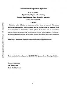
n FIG. 1: Probability distribution Wn over momentum eigenstates n in the quantum sawtooth map (3) at time t = 30. The quantum evolution is simulated by the quantum algorithm with nq = 6 qubits in presence of dissipative decoherence. The dissipation rate √ per gate √ is Γ = 0.001 and the map parameters are k = 3, K = 2 with the total number of states N = 2nq = 64. The full curve represents the exact solution of the Lindblad equation (4). Symbols show the result of quantum trajectories computation with the number of trajectories M = 20(+), M = 50(o), M = 200(x), M = 1000(△). The initial state is n = 0. The logarithm is natural.

This evolution of ρ can be efficiently simulated by averaging over the M quantum trajectories which evolve according to the following stochastic differential equation for states |ψ α i (α = 1, · · · , M ): |dψ α i = −iHs |ψ α idt + −L†m Lm )|ψ α idt +

X m



1X † (hLm Lm iψ 2 m 

(5)

 q Lm − 1 |ψ α idNm , † hLm Lm iψ

where hiψ represents an expectation value on |ψ α i and dNm are stochastic differential variables defined in the same way as in [29] (see Eq.(10) there). The above equation can be solved numerically by the quantum Monte Carlo (MC) methods by letting the state |ψ α i jump to one of Lm |ψ α i/|Lm |ψ α i| states with probability dpm ≡ p |Lm |ψ α i|2 dt [29] or evolve to (1 − P α iH P ef f dt/~)|ψ i/ 1 − m dpm with probability 1 − m dpm . Then, the density matrix can be approximately expressed as ρ(t) ≈ h|ψ(t)ihψ(t)|i M =

M 1 X α |ψ (t)ihψ α (t)| , M α=1

(6)

where hiM represents an ensemble average over M quantum trajectories |ψ α (t)i. Hence, an expectation value of an operator O is given by hOi = T r(Oρ) ≈ hOiM .

3 0

10

-2

10

-4

f

10

γ

0

10 -6

10

-1

10 -8

10

Γeff

-2

10

-1

0

10

1

10 20

10 40

t

60

80

100

FIG. 3: Fidelity f as a function of iteration time t. The upper two curves are for Γ = 0.0005 and the lower two curves are for Γ = 0.001. Here M = 50, nq = 8, k = 2nq K/2π and K = −0.5 (full curves) K = 0.5 (dotted curves), respectively. The initial state is |n = 0i. The inset shows the fidelity decay rate γ as a function of Γef f ≡ nq ng Γ with nq = 4, 6, 8. Here K = 0.5 (+) and K = −0.5(△), respectively. The straight line is the best fit γ = 0.08 Γef f .

FIG. 2: (Color online) First top row: classical phase space distribution obtained from the classical sawtooth map with a Gaussian averaging over a quantum cell (N = 256 quantum cells inside whole classical area; see text). Second row: the corresponding Husimi function for the quantum sawtooth map at nq = 8 and Γ = 0. Third row: the Husimi function obtained with M = 50 quantum trajectories in presence of dissipative decoherence with rate Γ = 0.0005 and nq = 8. Fourth bottom row: same as for the third row but with nq = 10. Here K = −0.5, T = 2π/N corresponding to L = 1 and N = 2nq quantum states in the whole classical area. Columns show distributions averaged in the time intervals: 0 ≤ t ≤ 9 (left), 40 ≤ t ≤ 49 (middle), 90 ≤ t ≤ 99 (right). The initial state is n ≈ 0.1N . Color represents the density from blue/black (0) to red/gray (maximal value).

For the quantum sawtooth algorithm the dissipative noise is introduced in the quantum trajectory context (Eq. (6)) after each elementary quantum gate and calculated by the MC methods. The same physical process can be described by density matrix theory. The evolution of density matrix after single iteration of quantum sawtooth map is described by ρ′ = Uk UT ρUT† Uk† .

(7)

To include the dissipative noise effects the density matrix further evolves according to Eq. (4) with Hs = 0 between consecutive quantum gates composing Uk and UT . To test the accuracy of the method of quantum trajec-

tories we compare its results with the exact solution of the Lindblad equation for the density matrix ρ (4). The comparison is done for the case of dynamical localization of quantum chaos and is shown in Fig. 1. It shows that the dynamical localization is preserved at relatively weak dissipation rate Γ. It also shows that the quantum trajectories method correctly reproduces the exact solution of the Lindblad equation and that it is sufficient to use M = 50 trajectories to reproduce correctly the phenomenon of dynamical localization in presence of dissipative decoherence of qubits. To analyze the effects of dissipation rate Γ in a more quantitative way we start from the quasi-integrable case K = −0.5 with one classical cell L = 1 (T = 2π/N ). The classical phase space distribution, averaged over a time interval and a Gaussian distribution over a quantum cell with an effective Planck constant, is shown in Fig. 2 in the first top row (there are N = 2nq quantum cells inside the whole classical phase space). Such Gaussian averaging of the classical distribution gives the result which is very close to the Husimi function in the corresponding quantum case at Γ = 0 (Fig. 2, second row). We remind that the Husimi function is obtained by a Gaussian averaging of the Wigner function over a quantum ~ cell (see [38] for details). In our case the Husimi function h(θ, n) is computed through the wave function of each quantum trajectory and after that it is averaged over all M trajectories. The effect of dissipative decoherence with Γ = 0.0005 is shown in the third row of Fig. 2. At Γ = 0 the phase space distribution remains approximately stationary in time while for Γ > 0 it starts to spread so that at large times the typical structure of the classical phase space becomes completely washed out. This destructive pro-

4

2

1

10

10

ξ/ξ0

ξ

1

10

0

0

1

10

10

t

2

10

FIG. 4: (Color online) Dependence of the IPR ξ on time t at Γ = 0.001 and M = 50 shown by full curves for nq = 4 (green/gray curve), nq = 6 (blue/black curve), nq = 8 (black curve), bottom to top respectively. The dashed curves show the same cases at Γ = 0 (bottom dashed curve is for nq = 4, top dashed curve is for nq = 6 and nq = 8 where ξ values are practically √ √identical). Here the initial state is |n = 0i and k = 3, K = 2.

cess becomes more rapid with the increase of the number of qubits even if Γ remains fixed (Fig. 2, fourth bottom row). One of the reasons is that Γ is defined as a rate per gate and the number of gates ng = 3n2q + nq grows with nq . However, this is not the only reason as it shows the analysis of the fidelity decay. The fidelity f of quantum algorithm in presence of dissipative decoherence is defined as f (t) ≡ hψ0 (t)|ρ(t)|ψ0 (t)i ≈

1 X |hψ0 (t)|ψΓα (t)i|2 , (8) M α

where |ψ0 (t)i is the wave function given by the exact algorithm and ρ(t) is the density matrix of the quantum computer in presence of decoherence, both are taken after t map iterations. Here, ρ(t) is expressed approximately through the sum over quantum trajectories (see also [29]). The dependence of fidelity f (t) on time t is shown in Fig. 3. At relatively short time t < 50 the decay is approximately exponential f (t) ≈ exp(−γt). The decay rate γ is described by the relation γ = CΓef f = Cnq ng Γ ,

(9)

where C = 0.08 is a numerical constant (see Fig. 3 inset). The important result of Fig. 3 is that the decay of f (t) is not very sensitive to the map parameters. Indeed, it is not affected by a change of K which significantly modify the classical dynamics which is quasi-integrable at K = −0.5 and fully chaotic at K = 0.5. Another important result is that up to a numerical constant the relation (9) follows the dependence found in [29] for the quantum

10 -4 10

-3

10

-2

Γ

10

-1

10

FIG. 5: (Color online) Dependence of the ratio of ξ to its value ξ0 in the ideal algorithm on the dissipative decoherence rate Γ for nq = 4 (green/gray o), nq = 6 (blue/black x), nq = 8(black +) from bottom to top. The values ξ and ξ0 are averaged in the time interval 30 ≤ t ≤ 40. Other parameters are as in Fig. 4.

baker map. This shows that the dependence (9) is really universal. Its physical origin is rather simple. After one gate the probability of a qubit to stay in upper state drops by a factor exp(−Γ) for each qubit (we remind that Γ is defined as a per gate decay rate). The wave function of the total system is given by a product of wave functions of individual qubits that leads to the fidelity drop by a factor exp(−Cnq Γ) after one gate and exp(−Cnq ng Γ) after ng gates leading to the relation (9). In principle, one may expect that the decay of f (t) is sensitive to a number of qubit up states in a given wave function since there is no decay for qubit down states. However, in a context of a concrete algorithm this number varies in time and only its average value contributes to the global fidelity decay. The result (9) gives the time scale tf of reliable quantum computation in presence of dissipative decoherence. On this scale the fidelity should be close to unity (e.g. f = 0.9) that gives tf ≈ 1/(nq ng Γ) ; Ng = 1/(nq Γ) .

(10)

Here Ng = ng t is the total number of quantum gates which can be performed with high fidelity (f > 0.9) at given nq and Γ. The comparison with the results obtained for static imperfections [21] of strength ǫ shows that for them Ng drops more rapidly with nq : Ng ∼ 1/(ǫ2 nq ng ). Therefore the static imperfections destroy the accuracy of quantum computation in a more rapid way compared to dissipative decoherence. It is also interesting to analyze the effects of dissipative decoherence on the dynamical localization. For that, in addition to the probability distribution as in Fig. 1, it is convenient to usePthe inverse participation ratio (IPR) P defined as ξ = 1/ n |ψn |4 ≃ 1/ n |h|ψn |2 iM |2 where

5 introduces some noise which destroys localization. However, there is also another effect which becomes visible at relatively large Γ. It is shown in Fig. 5 which gives the ratio of ξ to its value ξ0 in the ideal algorithm. Thus, at small Γ the ration ξ/ξ0 grows with the increase of Γ while it stars to drop at large Γ. This is a manifestation of the fact that in absence of algorithm the dissipation drives the quantum register to the state |n = 0i with all qubits in down state. Even in presence of the quantum algorithm this dissipative effect becomes dominant at large Γ leading to a decrease of the ratio ξ/ξ0 .

FIG. 6: (Color online) Each panel shows the Husimi distribution for the quantum sawtooth map algorithm with K = 1, T = 2π/2nq and nq = 8. The top three rows show the cases with the rate Γ = 0.01, Γ = 0.05, and Γ = 0.1, respectively from top to third row. The initial state is |n = 60i and M = 50. The distribution is averaged in the time interval 0 ≤ t ≤ 9 (left column), 40 ≤ t ≤ 49 (middle column), 90 ≤ t ≤ 99 (right column). The fourth bottom row shows the distribution for another initial state |n = 0i averaged in the time interval 90 ≤ t ≤ 99 for Γ = 0.01 (left panel), Γ = 0.05 (middle panel) , and Γ = 0.1 (right panel) (compare with the right column of top three rows). Color represents the density from blue/black (0) to red/gray (maximal value).

h| · · · |iM notes the average over M quantum trajectories. This quantity is often used in the problems with localized wave functions. In fact ξ gives an effective number of states over which the total probability is distributed. The dependence of ξ on time t is shown in Fig. 4. It shows that in presence of dissipative decoherence the dynamical localization is destroyed. Indeed, at large t the value of ξ grows with nq while for the ideal algorithm it is independent of nq . The physical meaning of this effect is rather clear. As in Fig. 2 the dissipative decoherence

[1] M.A. Nielsen and I.L. Chuang Quantum Computation and Quantum Information, Cambridge Univ. Press,

The dissipative effect of decoherence at large values of Γ is also clearly seen in the case of quantum chaos ergodic in one classical cell (L = 1). At large Γ the Husimi distribution relaxes to the stationary state induced by dissipation |n = 0i (third row in Fig. 6 at Γ = 0.1). In a sense this corresponds to a simple attractor in the phase space. The stationary state becomes more complicated with a decrease of Γ (second row in Fig. 6 at Γ = 0.05). And at even smaller Γ = 0.01 the stationary state shows a complex structure in the phase space (top first row in Fig. 6). It is important to stress that this structure is independent of the initial state (bottom row in Fig. 6). In this sense we may say that in such a case the dissipative decoherence leads to appearance of a quantum strange attractor in the quantum algorithm. Of course, this stationary quantum attractor state is very different from the Husimi distribution generated by the ideal quantum algorithm. However, it may be of certain interest to use the dissipative decoherence in quantum algorithms for investigation of quantum strange attractors which have been discussed in the context of quantum chaos and dissipation (see e.g. Refs. [39, 40, 41]). At the same time we should note that the dissipation induced by decoherence acts during each gate that makes its effect rather nontrivial due to change of representations in the map (3). In conclusion, our studies determine the fidelity decay law in presence of dissipative decoherence which is in agreement with the results obtained in [29] for a very different quantum algorithm. This confirms the universal nature of the established fidelity decay law. These studies also show that at moderate strength the dissipative decoherence destroys dynamical localization while a strong dissipation leads to localization and appearance complex or simple attractor. The effects of dissipative decoherence are compared with the effects of static imperfections and it is shown that in absence of quantum error correction the later give more restrictions on the accuracy of quantum computations with a large number of qubits. This work was supported in part by the EU IST-FET project EDIQIP.

Cambridge (2000).

6 [2] W.H. Zurek, Rev. Mod. Phys. 75, 715 (2003). [3] B. Georgeot, and D. L. Shepelyansky, Phys. Rev. E 62, 3504 (2000); ibid. 62, 6366 (2000). [4] D. L. Shepelyansky, Physica Scripta T90, 112 (2001). [5] J.I. Cirac and P. Zoller, Phys. Rev. Lett. 74, 4091 (1995). [6] C. Miquel, J. P. Paz and R. Perazzo, Phys. Rev. A 54, 2605 (1996). [7] C. Miquel, J.P. Paz and W.H. Zurek, Phys. Rev. Lett. 78, 3971 (1997). [8] P.H.Song and D.L.Shepelyansky, Phys. Rev. Lett. 86, 2162 (2001). [9] B. Georgeot and D.L. Shepelyansky, Phys. Rev. Lett. 86, 5393 (2001); ibid. 88, 219802 (2002). [10] A.D. Chepelianskii, and D.L. Shepelyansky, Phys. Rev. A 66, 054301 (2002). [11] D. Braun, Phys. Rev. A 65, 042317 (2002). [12] M. Terraneo, B. Georgeot and D.L. Shepelyansky, Eur. Phys. J. D 22, 127 (2003). [13] P.H. Song and I. Kim, Eur. Phys. J. D 23, 299 (2003). [14] B. L´evi, B. Georgeot and D.L. Shepelyansky, Phys. Rev. E 67, 046220 (2003). [15] S. Bettelli and D.L. Shepelyansky, Phys. Rev. A 67, 054303 (2003). [16] S. Bettelli, Phys. Rev. A 69, 042310 (2004). [17] G. Benenti, G. Casati, S. Montangero and D. L. Shepelyansky, Phys. Rev. Lett. 87, 227901 (2001). [18] M. Terraneo and D.L. Shepelyansky, Phys. Rev. Lett. 90, 257902 (2003). [19] G. Benenti, G. Casati, S. Montangero and D. L. Shepelyansky, Phys. Rev. A 67, 52312 (2003). [20] A.A. Pomeransky, D.L. Shepelyansky, Phys. Rev. A 69, 014302 (2004). [21] K. Frahm, R.Fleckinger and D.L.Shepelyansky, Eur. Phys. J. D 29, 139 (2004). [22] A.A. Pomeransky, O.V.Zhirov and D.L. Shepelaynsky, Eur. Phys. J. D 31, 131 (2004). [23] B. L´evi and B. Georgeot, Phys. Rev. E 70, 056218 (2004).

[24] B. V. Chirikov, in Chaos and Quantum Physics, Les Houches Lecture Series 52 Eds. M.-J. Giannoni, A.Voros, and J. Zinn-Justin (North-Holland, Amsterdam, 1991), p.443; F. M. Izrailev, Phys. Rep. 196, 299 (1990). [25] R. Schack, Phys. Rev. A 57, 1634 (1998). [26] B. Georgeot, and D.L. Shepelyansky, Phys. Rev. Lett. 86, 2890 (2001). [27] Y.S. Weinstein, S. Lloyd, J. Emerson, and D.G. Cory, Phys. Rev. Lett. 89, 157902 (2002). [28] G.G. Carlo, G. Benenti and G. Casati, Phys. Rev. Lett. 91, 257903 (2003). [29] G.G. Carlo, G. Benenti, G. Casati and C. MejiaMonasterio, Phys. Rev. A 69, 062317 (2004). [30] G. Lindblad, Commun. Math. Phys. 48, 119 (1976); Gorini, A. Kossakowski, and E.C.G. Sudarshan, J. Math. Phys. 17, 821 (1976). [31] H.J. Carmichel, An Open Systems Approach to Quantum Optics (Springer, Berlin, 1993). [32] R. Dum, P. Zoller, and H. Ritsch, Phys. Rev. A 45, 4879 (1992). [33] J. Dalibard, Y. Castin, and K. Mølmer, Phys. Rev. Lett. 68, 580 (1992). [34] N. Gisin, Phys. Rev. Lett. 52, 1657 (1984). [35] R. Schack, T.A. Brun, and I.C. Percival, J. Phys. A 28, 5401 (1995). [36] A. Barenco, T.A. Brun, R. Schack, and T.P. Spiller, Phys. Rev. A 56, 1177 (1997). [37] T.A. Brun, Am. J. Phys. 70, 719 (2002); quant-ph/0301046. [38] S.-J. Chang and K.-J. Shi, Phys. Rev. A 34, 7 (1986). [39] T. Dittrich and R. Graham, Annals of Physics 200, 363 (1990). [40] G. Casati, G. Maspero and D.L. Shepelyansky, Physica D 131, 311 (1999). [41] G. Carlo, G. Benenti, G. Casati and D.L. Shepelyansky, cond-mat/0407702.