Quantum circuit implementation of the Hamiltonian versions of

Quantum circuit implementation of the Hamiltonian versions of Grover’s algorithm J´er´emie Roland and Nicolas J. Cerf Ecole Polytechnique, CP 165/59, Universit´e Libre de Bruxelles, 1050 Brussels, Belgium (Dated: February 1, 2008)

arXiv:quant-ph/0302138v1 19 Feb 2003

We analyze three different quantum search algorithms, the traditional Grover’s algorithm, its continuous-time analogue by Hamiltonian evolution, and finally the quantum search by local adiabatic evolution. We show that they are closely related algorithms in the sense that they all perform a rotation, at a constant angular velocity, from a uniform superposition of all states to the solution state. This make it possible to implement the last two algorithms by Hamiltonian evolution on a conventional quantum circuit, while keeping the quadratic speedup of Grover’s original algorithm.

I.

INTRODUCTION

While the standard paradigm of quantum computation uses quantum gates (i. e., unitary operators) applied sequentially on a quantum register, recent developments have introduced a new type of quantum algorithms where the state of the quantum register evolves continuously in time under the action of some Hamiltonian. It includes, for instance, the “analog analogue” of Grover’s algorithm [1] or the quantum algorithms by adiabatic evolution that have been intensively studied lately [2, 3]. It has been shown that these Hamiltonian algorithms are genuinely quantum in the sense that they reproduce the quadratic speed-up of Grover’s algorithm (see, in particular, the local adiabatic version of Grover’s algorithm [3, 4]). The purpose of this paper is, on one hand, to clarify the links between these Hamiltonian algorithms and their conventional discrete equivalents, and, on the other hand, to show how they can be implemented on a traditional quantum circuit. This second issue is important because it was never shown before how it could be done keeping the quadratic speed-up of Grover’s algorithm. It appears that all these algorithms take a very similar form in the high dimension limit, which is particularly surprising for the case of the adiabatic search algorithm. Specifically, we see that the mixing parameter (which measures the mixing between the initial and final Hamiltonians in the adiabatic search algorithm) has to evolve in such a way that the instantaneous ground state rotates at a constant rate from the initial to the final ground state. This makes the link fully explicit with Grover’s original algorithm. II.

TRADITIONAL GROVER’S ALGORITHM

First of all, let us briefly recall the principle of Grover’s algorithm [5, 6]. It is designed to solve the problem of finding the values x for which a function f (x), usually called the “oracle”, is equal to 1 (while it vanishes everywhere else). As quantum gates have to be reversible, the quantum oracle must take the form: Of : HN ⊗ H2 → HN ⊗ H2 : |xi ⊗ |yi → |xi ⊗ |y ⊕ f (x)i (1) where the N candidate solutions |xi are taken as the basis states of the Hilbert space HN , while ⊕ stands for the

addition modulo 2. By considering the second register H2 as an ancilla and preparing it in the state √12 [|0i − |1i], the application of Of on both registers will be equivalent to the following unitary operation on the first one: Uf : HN → HN : |xi → (−1)f (x) |xi

(2)

To clarify the notations, we will throughout this article restrict ourselves to the case where there is only one solution x = m (our results may easily be generalized to the case of M solutions, roughly speaking by replacing N by N/M in all the formulas below). In this case, f (m) = 1 while f (x) = 0 (∀x 6= m) and Uf may be rewritten Uf = I − 2|mihm|.

(3)

Initially, we have no idea of what the solution could be, so we prepare the system in a uniform superposition of all possible solutions: N −1 1 X |xi. |si = √ N x=0

(4)

This state may easily be obtained by applying an Hadamard transform H on the n = log2 N qubits realizing the quantum register HN , initially prepared in state |0i. The algorithm will also require the following operation: U0 = H ⊗n (I − 2|0ih0|)H ⊗n = I − 2|sihs|.

(5)

Let us define as a Grover iteration the operator G = −U0 Uf . Throughout this article, we will always assume that N ≫ 1 for simplicity reasons but also because the link between the different versions of the algorithm will appear much more clearly. In that limit, it may be shown that the Grover iteration becomes a simple rotation of angle √2N in the subspace spanned by |si and |mi. More precisely, successive applications of G on the initial state |si will progressively make this state rotate to the solution state |mi: 2j 2j |ψjdis i = Gj |si ≈ cos √ |si + sin √ |mi N N dis ≈ cos αdis |si + sin α j j |mi

(6) (7)

2 where αdis j

2j =√ . N

(8)

√ Thus, by applying the Grover iteration Rdis ≈ π4 N times, we obtain the solution state |mi with a probability close to 1 with a quadratic speed-up with respect to a classical search, which would necessarily require a number of calls to the oracle f (x) of order N . √ Let us notice that as π4 N is generally not an integer, we have to round it, for √ instance to the nearest lower integer, so that Rdis = ⌊ π4 N ⌋. This results in an error 2 2 dis k|ψR ≈√ dis i − |mik < sin √ N N

(9)

HAMILTONIAN EQUIVALENT OF THE ORACLE

In the two Hamiltonian quantum search algorithms discussed below, we will use the Hamiltonian: Hf = I − |mihm|.

e

−iHf t

|xi =

|xi x=m e−it |xi ∀x = 6 m.

= e−i(1−f (x))t |xi.

(11) (12)

We immediately see that by taking t = π, we reproduce the operation −Uf , that is e−iHf π = −Uf

(13)

Conversely, it is possible to simulate the application of Hf during a time t by a quantum circuit using a onequbit ancilla prepared in state |0i, two calls to the oracle Of and an additional phase gate Ut = e−it |0ih0| + |1ih1|.

(14)

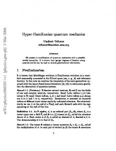
Considering the circuit represented in Fig. 1), we have Of [|xi ⊗ |0i] = |xi ⊗ |f (x)i

I ⊗ Ut [|xi ⊗ |f (x)i] = e−i(1−f (x))t |xi ⊗ |f (x)i h i Of e−i(1−f (x))t |xi ⊗ |f (x)i = e−i(1−f (x))t |xi ⊗ |0i = e−iHf t |xi ⊗ |0i.

Of

|0i

Ut

e−iHf t |xi |0i

FIG. 1: Circuit for implementing the evolution of a Hamiltonian Hf during a time t by using twice the corresponding oracle Of .

IV.

ANALOG QUANTUM SEARCH

Let us now consider the “analog” algorithm introduced by Farhi et al. in [1]. In addition to the oracle Hamiltonian Hf , we will need a second Hamiltonian

(15)

(16)

that is related to U0 as defined in Eq. (5) in the same manner than Hf is related to Uf . The algorithm consists in preparing the system in the starting state |ψ an (t = 0)i = |si and then let it evolve under the timeindependent Hamiltonian H an = H0 +Hf . We may show by simple calculation that: |ψ an (t)i = e−iH

an

t

|si (17) t t = e−it [cos √ |si + i sin √ |mi] (18) N N = e−it [cos αan (t)|si + i sin αan (t)|mi], (19)

(10)

Let us show why it can be considered as equivalent to the oracle Uf . If we apply this Hamiltonian on a basis state |xi during a time t, it yields 

Of

H0 = H ⊗n (I − |0ih0|)H ⊗n = I − |sihs|

that tends to zero for N → ∞. III.

|xi

where t αan (t) = √ . N

(20)

As in the traditional algorithm, the search works via a rotation from |si to |mi. However, the rotation is continuous here, and follows a different path because of the presence of i in the second term of Eq. (19). The solution state is thus obtained with√probability one if we apply H an during a time T an = π2 N . Let us also notice that αan (2j) = αdis j

(21)

which shows that the application of H an during a time T an /Rdis = 2 corresponds roughly to one Grover iteration. Suppose now we want to implement this analog algorithm on a quantum circuit. We showed in the previous section how to reproduce the application of Hf with a circuit, but this does not allow us to directly apply H an = H0 + Hf . In order to achieve this, we need to cut the evolution time T an into Ran small intervals √ T an π N ∆T = Ran = 2 Ran such that we may approximate U (∆T ) = e−i(H0 +Hf )∆T

(22)

′ U∆T = e−iH0 ∆T e−iHf ∆T .

(23)

by

3 Using the Campbell-Baker-Hausdorff approximation, which states that |||eA+B − eA eB |||2 ∈ O(|||[A, B]|||2 ) with |||A|||2 = maxk|xik=1 kA|xik denoting the operator norm of A, we have ′ |||U (∆T ) − U∆T |||2 ∈ O(|||[H0 , Hf ]|||2 ∆T 2 ).

(24)

As [H0 , Hf ] =

r

1 N

r

1−

1 1 . √ , N N

the error introduced at each step is of order √ N ′ |||U (∆T ) − U∆T |||2 ∈ O( an 2 ) R

(25)

(26)

Let us first study the path followed by |ψ ad (t)i during the evolution. As H(s) only acts on the subspace spanned by |si and |mi and as we start from |si, the path followed by |ψ ad (t)i will remain in this subspace so that the problem may be studied in this 2-dimensional Hilbert space. By calculating the eigenstates of H(s), we find √ N (E1 (s) − s)|si + s|mi |E0 ; si = p (30) E1 (s)2 + (N − 1)(E1 (s) − s)2 √ N (E0 (s) − s)|si + s|mi |E1 ; si = p (31) E0 (s)2 + (N − 1)(E0 (s) − s)2 where

" # r N −1 1 1− 1−4 s(1 − s) E0 (s) = 2 N " # r 1 N −1 E1 (s) = 1+ 1−4 s(1 − s) . 2 N

Since there are Ran successive steps, the global error made by this discretized analog algorithm is √ an N ′ (27) |||U (T ) − (U∆T )R |||2 ∈ O( an ). R This simply results from the property that if the condition |||Uj − Uj′ |||2 ≪ 1 is fulfilled ∀j, then |||

Y j

Uj −

Y j

Uj′ |||2 ≤

X j

|||Uj − Uj′ |||2 .

(28) √

We thus observe that for a number of steps Ran = ⌊ ǫN ⌋ (of the same order in N as in Grover’s traditional algorithm), we get the desired state with an error of order ǫ. Furthermore, keeping the results of the previous section in mind, each step will have the same form e−iH0 δT e−iHf δT as a Grover iteration G = −U0 Uf , and therefore will require 2 calls to the oracle Of for being implemented with a quantum circuit.

V.

QUANTUM SEARCH BY LOCAL ADIABATIC EVOLUTION

H(s) = (1 − s)H0 + sHf

(29)

to the system, where the mixing parameter s = s(t) is a monotonic function with s(0) = 0 and s(T ad ) = 1. As |si is the ground state of H(0) = H0 , the Adiabatic Theorem [7] tells us that during the evolution s(t), the system will stay near the instantaneous ground state of H(s) as long as the evolution of H(s) is slow enough. If this condition is satisfied, the system will thus end up in the ground state of H(1) = Hf , which is the solution state |mi.

(33)

If the adiabatic condition is realized (see [4]), we have √ N (E1 (s) − s)|si + s|mi ad (34) |ψ (s)i ≈ p E1 (s)2 + (N − 1)(E1 (s) − s)2 ≈ cos αad (s)|si + sin αad (s)|mi

(35)

where s αad (s) = arctan √ N (E1 (s) − s) 1 2s ≈ arctan √ 2 N (1 − 2s)

(36) (37)

in the limit N ≫ 1. π/2

αad (s)

For this third algorithm, exposed in [3] and [4], we will once more need the Hamiltonians H0 and Hf , and we will initially prepare our system in a uniform superposition of all possible solutions |ψ ad (t = 0)i = |si. This time, however, we apply a time-dependent Hamiltonian

(32)

π/4

0

0

0.5

1

s FIG. 2: Rotation angle αad (s) for the adiabatic quantum search algorithm with N = 32.

The function αad (s) is plotted in Fig. 2. We see that the evolution is once again a rotation from |si to |mi, but which is not performed at a constant angular velocity if s(t) is chosen to be linear in t, which corresponds to the quantum search by global adiabatic evolution originally described in [2]. The observed angular velocity is

4 indeed greater for s close to 1/2 while it is smaller at the beginning and the end of the time evolution. Let us also notice that at discrete values s(t) = sk , the continuous path |ψ ad (s)i coincides with the states |ψjdis i of Grover’s traditional algorithm. Thus, in the global adiabatic search algorithm, the system exactly follows the path of Grover’s algorithm, but at a varying rate. This suggests that this algorithm is not the correct adiabatic equivalent to Grover’s algorithm. Moreover, we note that if s(t) = t/T ad , then the Adiabatic Theorem imposes that T ad ∈ O(N ), so that we loose the quadratic speed-up of Grover’s algorithm (see [4]). In order to circumvent this problem, we can perform a local adiabatic evolution as defined in [4]. Then we get the solution state with an error less than ǫ k|ψ ad (T ad )i − |mik ≤ ǫ

(38)

the Hamiltonian difference δ(t) may vary in time. This will be crucial in order to keep the quadratic speedup of Grover’s search after this discretization procedure (this is reminiscent to the distinction between the global and the local adiabatic evolution). The proof of Lemma 1 is left to the reader. Thus, the approximation we made is equivalent to replacing the actual Hamiltonian H(t) = H(s(t)) by H ′ (t) = H(s′ (t)) where s′ (t) is a new monotonic function approaching s(t) but varying at times tj only (see Fig. 3). 1

s′ (t) s(t)

0.5

provided that we evolve at a rate such that √ N √ [arctan[ N − 1(2s − 1)] 2ǫ N − 1 √ + arctan N − 1] √ √ N − 1(2s − 1) + N − 1 N √ arctan = 1 − (N − 1)(2s − 1) 2ǫ N − 1 √ 2s N arctan √ ≈ (39) 2ǫ N (1 − 2s)

t(s) =

in the limit N ≫ 1. Thus, for a local adiabatic evolution, ǫt αad (t) ≈ √ . N

(40)

This is now √ a rotation at a constant rate during a time π N , so that we may consider this local adiaT ad = 2ǫ batic evolution as the right equivalent to Grover’s algorithm. Let us study the implementation of this algorithm on a quantum circuit (we will closely follow the lines of the development exposed in [3]). As for the analog quantum search, we discretize the evolution by cutT ad ting the time T ad in Rad intervals ∆T = R Durad . ing each interval [tj−1 , tj ](tj = j∆T ), we approximate the varying Hamiltonian H(s(t)) by the constant one Hj = (1 − sj )H0 + sj Hf (sj = s(tj )). In order to evaluate the error introduced by this approximation, we will use the following lemma: Lemma 1 Let H(t) and H ′ (t) be two time-dependent Hamiltonians for 0 ≤ t ≤ T , and let U (T ) and U ′ (T ) be the respective unitary evolutions that they induce. If the difference between the Hamiltonians is limited by |||H(t) − H ′ (t)|||2 ≤ δ(t), then the distance between the in′ duced q R transformations is bounded by |||U (T ) − U (T )|||2 ≤ T 2 0 δ(t)dt. This lemma is a straightforward generalization of the one introduced in [3], with the important difference that

0

0

T ad /2

T ad

t FIG. 3: s(t) and its discrete approximation s′ (t) (using Rad = 20 steps) for the local adiabatic algorithm with N = 32.

We have |||H(t) − H ′ (t)|||2 = |||H(s(t)) − H(s′ (t))|||2 (41) = |s′ (t) − s(t)| |||Hin − Hf |||2 (42) ds ≤ ( ∆T + O(∆T 2 ))|||Hin − Hf |||2 . dt We may use Lemma 1 with δ(t) = Z

0

ds dt ∆T |||Hin

T

δ(t)dt = ∆T |||Hin − Hf |||2 = ∆T |||Hin − Hf |||2 = ∆T |||Hin − Hf |||2 ≤ ∆T

Z

T

0

Z

− Hf |||2 :

ds dt dt

(43)

1

ds

(44)

0

(45) (46)

as we may easily see that |||Hin − Hf |||2 ≤ 1. Now, the lemma gives: r √ T ad ′ (47) |||U (T ) − U (T )|||2 ≤ 2∆T = 2 ad R so that in order to keep an error of constant order ǫ for growing N , we must choose a √number of steps proportionnal to T ad , that is Rad = ⌊ ǫ3N ⌋. For each step, we have to apply Hj during a time ∆T = T ad , that is the unitary operation: Rad Uj′ = e−iHj ∆T = e−i(1−sj )H0 ∆T −isj Hf ∆T .

(48)

5 Grover √ ⌊ π4 N ⌋

#steps R Step j State |ψj i Angle αj

Analog √ ⌊ ǫN ⌋

(

Adiabatic √ ⌊ ǫ3N ⌋

δt0,j = (1 − sj )ǫ2 π2 δtf,j = sj ǫ2 π2 cos αj |si + sin αj |mi cos αj |si + i sin αj |mi cos αj |si + sin αj |mi δt0,j = δtf,j = π

Error k|ψR i − |mik

2j √ N O( √1N )

δt0,j = δtf,j =

ǫ π2

√ǫj π N 2

ǫ3 j π √ N 2

O(ǫ)

O(ǫ)

TABLE I: Summary of the properties of the three quantum search algorithms. Here δt0,j and δtf,j are the times during which H0 and Hf have to be applied in step j. Notice that we have omitted some irrelevant global phases in front of |ψj i and |ψR i

As for the analog algorithm, we use the Campbell-BakerHausdorff approximation and replace Uj′ by Uj′′ = e−i(1−sj )H0 ∆T e−isj Hf ∆T .

(49)

The error introduced at each step by this approximation will be √ N ′ ′′ |||Uj − Uj |||2 ∈ O(sj (1 − sj ) (50) 2 ). ad R Q For the Rad steps we have U ′ (T ) = j Uj′ , so that using Eq. (28) gives √ Y N ′ ′′ |||U (T ) − Uj |||2 ∈ O( ad ) (51) R j

that have been found so far are very closely related. They all perform a rotation from the uniform superposition of all states to the solution state at a constant angular velocity, even though a slightly different path is followed by the analog quantum search algorithm. Their similarities become even more obvious when they are implemented on a quantum √ circuit as they all require a number of steps of order N , each step having the same form e−iH0 δt0 e−iHf δtf . Note that the “duty cycle” δtf /(δt0 + δtf ) varies along the evolution according to a specific law in the case of the local adiabatic search algorithm. Finally, we have shown how one can realize these basic steps on a quantum circuit by using two calls to the quantum oracle. These results are summarized in Table I.

√

Consequently, the number of steps Rad = ⌊ ǫN 3 ⌋ required in the previous approximation (i.e., replacing H(t) by H ′ (t)) results in an error of order ǫ3 here. Acknowledgments VI.

CONCLUSION

We have shown that, in spite of their different original implementations, the three quantum search algorithms

[1] E. Farhi and S. Gutmann, Phys. Rev. A 57, 2403 (1998), e-print quant-ph/9612026. [2] E. Farhi, J. Goldstone, S. Gutmann, and M. Sipser (2000), e-print quant-ph/0001106. [3] W. van Dam, M. Mosca, and U. Vazirani, in Proceedings of the 42nd Annual Symposium on the Foundations of Computer Science (IEEE Computer Society Press, New York, 2001), pp. 279–287. [4] J. Roland and N. J. Cerf, Phys. Rev. A 65, 042308 (2002),

J.R. acknowledges support from the Belgian foundation FRIA. N.J.C. is funded in part by the project RESQ under the IST-FET-QJPC European programme.

e-print quant-ph/0107015. [5] L. K. Grover, in Proceedings of the 28th Annual Symposium on the Theory of Computing (ACM Press, New York, 1996), pp. 212–219. [6] L. K. Grover, Phys. Rev. Lett. 79, 325 (1997). [7] L. I. Schiff, Quantum Mechanics (Mc Graw-Hill, Singapore, 1955).