Quantum coding theorems

Home

Search

Collections

Journals

About

Contact us

My IOPscience

Quantum coding theorems

This content has been downloaded from IOPscience. Please scroll down to see the full text. 1998 Russ. Math. Surv. 53 1295 (http://iopscience.iop.org/0036-0279/53/6/R04) View the table of contents for this issue, or go to the journal homepage for more

Download details: IP Address: 181.215.97.173 This content was downloaded on 31/10/2016 at 13:40

Please note that terms and conditions apply.

You may also be interested in: Quantum channels and their entropic characteristics A S Holevo and V Giovannetti Determinantal random point fields A Soshnikov The continuity of the output entropy of positive maps Maxim E Shirokov Joint sessions of the Petrovskii Seminar and the Moscow Mathematical Society (nineteenth session, 20-24 January 1998)

Controlled random sequences: methods of convex analysis and problems with functional constraints A B Piunovskii Reversibility conditions for quantum channels and their applications M E Shirokov On the small balls problem for equivalent Gaussian measures V I Bogachev

Russian Math. Surveys 53:6 1295–1331 Uspekhi Mat. Nauk 53:6 193–230

c

1998 RAS(DoM) and LMS UDC 519.723

Quantum coding theorems

A. S. Holevo Contents I. Introduction II. General considerations §1. Quantum communication channel §2. Entropy bound and channel capacity §3. Formulation of the quantum coding theorem. Weak conversion III. Proof of the direct statement of the coding theorem §1. Channels with pure signal states §2. Reliability function §3. Quantum binary channel §4. Case of arbitrary states with bounded entropy IV. c-q channels with input constraints §1. Coding theorem §2. Gauss channel with one degree of freedom §3. Classical signal on quantum background noise Bibliography

1295 1296 1296 1299 1303 1304 1304 1308 1309 1311 1314 1314 1318 1321 1329

I. Introduction In the wake of the pioneering investigations of Shannon fifty years ago and the elaboration of the mathematical foundations of information theory (see, for example, [17]), the question comes to mind of such fundamental restrictions on the possibilities of information transmission as are imposed by the physical nature of the information carrier. The problem of estimating the channel capacity of a quantum communication channel achieved a definitive form in the 1960s (see, for example, [13], [10], [34], [14], and the survey [7]). This dates back to earlier classical works by Gabor and Brillouin who proposed the task of finding quantum-mechanical limit values for the accuracy and rate of information transmission. These investigations laid the physical foundations for and kindled an interest in the adequate mathematical study of all these topics. Crucial progress along this line of inquiry was made in the 1970s, when (1) the non-commutative theory of statistical decisions was developed [16], [21], (2) the existence of the quantum entropy bound This work was carried out with the partial support of the Russian Foundation for Fundamental Research (grant nos. 96-01-01709 and 96-15-96033.).

1296

A. S. Holevo

was established [19], and (3) the strict superadditivity of Shannon information was shown for memory-free quantum communication channels [24]. A notable advance has been made in recent years, when direct coding theorems were proved which show that the quantum entropy bound is attained [15], [26], [42]. This progress was stimulated to some extent by the modern development of quantum information theory and the theory of quantum computing (see, for example, [4]). The question of the channel capacity of a quantum communication channel is of great interest in connection with the recent discovery of quantum error-correcting codes [6], [43]. It should be remembered that here the classical and quantum channel capacities of a quantum communication channel are different. As to the quantum channel capacity, which gives a characterization of the process of asymptotically error-free transmission of quantum states and is of a fundamental interest in quantum computing, we have as yet no steady-state definition. Some important results along this line are presented in [2] and [1], where an upper bound is suggested; however, the question whether this bound is attained remains unsolved. In this paper we give a self-contained and mathematically rigorous presentation of a range of problems connected with the classical channel capacity of a quantum channel, which is defined as the maximum amount of Shannon information that can be asymptotically transmitted without error via a quantum communication channel using an arbitrary block coding. This material is of interest in its own right and at the same time is a necessary step in passing from classical information theory to the quantum case. Prominence is given to recent achievements, the history of the problem is briefly reviewed, and a number of unsolved problems are posed. II. General considerations §1. Quantum communication channel From the mathematical point of view, a communication channel is an affine mapping that takes input channel states to output ones. The states are regarded as statistical ensembles, which may be subjected to mixing, and the affineness expresses a fundamental property of conservation of statistical mixtures. In the classical case, states are described by probability distributions, and a classical communication channel is defined as a mapping of input distributions onto output ones. If at least one of these input-output systems is quantum then the communication channel is called a quantum channel. Let be a separable Hilbert space giving the mathematical description of a physical information carrier. We do not suppose that the is finite-dimensional, as is usual in quantum computing problems, since this assumption breaks down, for example, in the case of the Gauss channel (see § IV.3). In this context, a quantum state is given by a density operator, that is, by a positive operator S of unit trace in , Tr S = 1. Following the Dirac formalism, we denote vectors of by |ψi, and Hermitian conjugate vectors of the dual space by hψ|. Then we denote by hφ|ψi the scalar (inner) product of vectors |φi, |ψi, and by |ψihφ| the exterior product, that is, the operator A of rank 1 acting on a vector |χi by the rule A|χi = |ψihφ|χi. If |ψi is a unit vector, then |ψihψ| is the

H

H

H

H

Quantum coding theorems

1297

orthogonal projection onto |ψi. In this particular case the density operator represents a pure state of the system. Pure states are extreme points of the convex set ( ) of all states. An arbitrary quantum state S can be represented by a mixture of pure states. Indeed, the spectral theorem for completely continuous operators implies that X S= λi |ψiihψi |,

SH

i

where λi and |ψi i are eigenvalues and eigenvectors of the operator S, respectively (the series converges in the trace class norm). We note that the {λi } form a probability distribution, that is, a classical state on the spectrum of S. On the other hand, given a fixed orthonormal basis {|ψii} in , any (discrete) classical state can be thus affinely embedded in ( ). The next important concept is the quantum decision rule, which is a far-reaching generalization of the standard definition of a quantum observable. In mathematical terms it is described as a partition of unity in a Hilbert space , that is, as a family P X = {Xj } of positive-definite operators in such that j Xj = I, where I is the identity operator in . We arrive at the standard definition of observable if we further assume that Xj are mutually orthogonal projections, Xj Xk = δjk Xj . The famous theorem of Naimark [39] states that any partition of unity can be extended to an orthogonal one in some enveloping Hilbert space. From a physical point of view, this means that any decision rule is equivalent to the measurement of an observable in some extension of the original quantum system [25]. The probability of taking a decision j for the decision rule X applied to a system in a state S is, by definition, P (j|S) = Tr SXj .

SH

H

H

H

H

This relation becomes the statistical Born postulate for an ordinary observable, which in turn is equivalent to the Born formula for an observable of an extended system for which the decision rule X is realized. P A system of vectors {|φj i} of is called over lled in if j |φj ihφj | = I. Any overfilled system (in particular, any orthonormal basis) generates a decision rule X such that Xj = |φj ihφj | and P (j|S) = hφj |Sφj i. The mapping S → P ( · |S) is affine and, conversely, any affine mapping of a set of quantum states into probability distributions takes this form (see [25], Proposition 1.6.1). Such a mapping is in fact an example of a quantum channel (called a q-c channel, see (19)). The classical case fits in with this picture when the operators considered commute with each other, and therefore are of diagonal form in some basis indexed by a variable ω. Indeed, let us put S = diag[S(ω)], Xj = diag[X(j|ω)], where S(ω) and X(j|ω) are a classical state and P decision rule, respectively; then we arrive at the classical formula P (j|S) = ω X(j|ω)S(ω). Quantum observables thereby correspond to classical deterministic decision rules (that is, to random variables). In earlier investigations (see, for example, [9]), a quantum communication channel was defined as an arbitrary affine mapping Φ of the set ( ) of states. It is an easy matter to prove that such a mapping can be uniquely extended to a positivedefinite linear mapping of the Banach space of trace class operators in , and this mapping preserves the trace. Later it became clear that the positivity property in

H

H

SH

H

1298

A. S. Holevo

this definition must be essentially strengthened [18], [32], [38]. Let us call a linear the mapping Φ completely positive if for any finite set of vectors {|φii, |ψii} ⊂ inequality X hφi |Φ[|ψiihψj |]|φj i > 0 (1)

H

i,j

holds. (This is only one of a number of equivalent definitions.) A well-known result of Stinespring [44] (generalizing the theorem of Naimark cited above) states that a completely positive mapping can be extended to an algebra representation (in the case considered here, to a representation of the algebra of all bounded operators in ) in some enveloping space. In quantum physics, this is equivalent to the mapping generated by a unitary evolution of some enveloping system which includes an environment of the original system [32], [38]. Based on Stinespring’s theorem, it is easy to show that any completely positive mapping which preserves the trace and is continuous in the weak operator topology takes the form X Φ[S] = Vk SVk∗ , (2)

H

k

P where Vk are bounded operators such that k Vk∗ Vk = I. Hereafter we call such a mapping a channel.1 We consider two important particular cases. Let {Si } be a family of quantum states and {Xi } a partition of unity in . We set X Φ[S] = Si Tr SXi . (3)

H i

It is easy to verify that this mapping is completely positive and preserves the trace. If Xi = |ei ihei |, where {ei } is an orthonormal basis, then we call it a c-q (classically-quantum ) channel. The mapping is uniquely defined by the mapping i → Si of the input alphabet A = {i} onto the signal quantum states Si . If the operators Si commute with each other, then the channel is called quasiclassical ; any such channel is equivalent to the classical channel, whose transition probabilities are given by the eigenvalues S(ω|i) of the operators Si . On the other hand, if Xi is an arbitrary partition of unity and Si = |ei ihei |, then we call the channel a q-c (quantum-classical ) channel, since it is defined by a decision rule which maps quantum states into probability distributions on the output alphabet B = {i}. Needless to say, channels of the form (3) do not exhaust all possible cases. In particular, the simplest example which cannot be reduced to (3) is given by the invertible evolution Φ[S] = V SV ∗ ,

(4)

where V is an arbitrary unitary operator. 1 In

a recent paper [11] a more general definition is taken, which is free from the assumption of complete positivity. Similar efforts are of interest in the light of the recent observation [31] that positive but not completely positive mappings appear in models of interaction with a more complicated environment (such as a non-Abelian gauge field), and these are described in terms of operators in the graded (rather than ordinary) tensor product of Hilbert spaces.

Quantum coding theorems

1299

§2. Entropy bound and channel capacity

SH

Let π be a discrete probability distribution on ( ) ascribing the probability πi to the the state Si . We put ∆H(π) =

X

πiH(Si ; S π ),

(5)

i

where Sπ =

X

πi Si

(6)

i

and

H(S; S 0 ) = Tr S(log S − log S 0 )

is a relative quantum entropy (for a more precise definition and a discussion of properties of these quantitites see [38], [47], [40]). Like the relative entropy, the quantity ∆H(π) is non-negative but can be infinite. If sup H(Si ) < ∞,

(7)

i

where H(S) = − Tr S log S is von Neumann’s quantum entropy, then ∆H(π) = H(S π ) − H(S( · ) ),

(8)

P where H(S( · ) ) = i πiH(Si ) < ∞. Let X = {Xj } be a decision rule and P (j|i) = Tr Si Xj the corresponding transition probabilities. We denote by I(π, X) =

XX j

i

  P (j|i) πiP (j|i) log P k πk P (j|k)

(9)

the classical Shannon amount of information between the random variables describing the input and output of the communication channel. The following quantum entropy bound holds: sup I(π, X) 6 ∆H(π), (10) X

with equality if and only if the operators πi Si commute with each other. This inequality was first formulated in (14) as a conjecture within the framework of standard quantum measurement theory. In the finite-dimensional case, a proof was given in [19] based on an investigation of the convexity properties of the right- and left-hand sides in (10). Another approach to the proof of (10) is to use the “generalized H-theorem”, which was established later in the series of papers [38] and in [46]. This theorem is based on the strong subadditivity of the quantum entropy [37]. Namely, for any states S, S 0 and channel Φ, the following inequality holds: H(Φ(S); Φ(S 0 )) 6 H(S; S 0 ).

1300

A. S. Holevo

If we take Φ to be the q-c channel corresponding to the decision rule X, then this inequality can be used to establish the entropy bound in the most general case (see [48]). The original proof given in [19] can also be generalized to the infinite-dimensional case subject to the condition (7), and the reformulation of the entropy bound in terms of conditional entropy also makes it possible to cover the case when the condition (7) and the relation (8) break down (in particular, when the states Si may have infinite entropy.) Given a channel Φ, we denote by I(π, Φ, X) the amount of information defined as in (9) but inserting P (j|i) = Tr Φ[Si ]Xj for the transition probabilities, ∆H(π, Φ) =

X

πiH(Φ[Si ]; Φ[Sπ ]).

(11)

i

With the study of block coding in mind we introduce the tensor power Φ⊗n = Φ ⊗ · · · ⊗ Φ of a channel in the Hilbert space ⊗n = ⊗ · · · ⊗ . We put

H

Cn (Φ) = sup sup I(π, Φ⊗n , X); π

H

H

C n (Φ) = sup ∆H(π, Φ⊗n ),

(12)

π

X

where the suprema are taken over all possible discrete probability distributions π on ( ⊗n) and over all possible decision rules X in ⊗n. It is easy to see that the sequences Cn (Φ), C n (Φ) possess the superadditivity property

SH

H

Cn (Φ) + Cm (Φ) 6 Cn+m (Φ),

C n (Φ) + C m (Φ) 6 C n+m (Φ).

This implies the existence of the limits Cn (Φ) Cn (Φ) = sup , n n n C n (Φ) C n (Φ) C(Φ) = lim = sup . n→∞ n n n

C(Φ) = lim

n→∞

(13) (14)

Taking into account the entropy bounds, we obtain C(Φ) 6 C(Φ). For a (quasi-)classical channel, the sequence Cn (Φ) is additive, Cn (Φ) = nC1 (Φ), and, obviously, C(Φ) = C(Φ) = C1 (Φ). One of the most essential and important features peculiar to the quantum case is that the inequality C1 (Φ) < C(Φ) can occur, in which case the sequence Cn (Φ) is strictly superadditive. The paradox lies in the fact that quantum channels, which are natural generalizations of classical memory-free channels, have a specific “quantum memory.” This phenomenon can be interpreted as a dual manifestation of the well-known “Einstein–Podolskii–Rosen correlations” in quantum measurements over compound systems (for more detail see [26]). We call the value C(Φ) the channel capacity of the quantum channel. This definition can be justified by the classical Shannon coding theorem (see [24]),

Quantum coding theorems

1301

but we suggest another motivation, from which the following much more essential fact also emerges: (15) C(Φ) = C(Φ). In some cases (see the discussion below), the sequence C n (Φ) is liable to be additive. This makes it possible to get rid of the limit in (14) and enables us to calculate the channel capacity using the formula C(Φ) = C 1 (Φ) = sup ∆H(π, Φ). π

The problem of the additivity of this sequence was raised in [3]. In the general case this problem remains unsolved. The additivity is trivial for convertible channels (4). We now present a partial result of this kind. Proposition 1.

If Φ is a c-q or a q-c channel, then C n (Φ) + C m (Φ) = C n+m (Φ).

Proof.

It suffices to show that C 1 (Φ) + C 1 (Φ) > C 2 (Φ).

(16)

If Φ is a c-q channel, that is, Φ[S] =

X

Si hei |S|ei i,

(17)

i

where Si are fixed states in

H, then

sup ∆H(π, Φ) = sup ∆H(π), π

πi

where ∆H(π) is given by (5). Let us consider a distribution π that ascribes to the states Si ⊗ Sj in ⊗ the probabilities πij . Then

H H

∆H(π) 6 ∆H(π 1 ) + ∆H(π 2 ),

(18)

whereP π 1 is the first marginal distribution ascribing to the states Si the probabilities 1 πi = j πij and, similiarly, π 2 is the second marginal distribution ascribing to the P states Sj the probabilities πj2 = i πij . In the finite-dimensional case (when the relation (8) holds automatically), the validity of (18) follows from the property that entropy is subadditive with respect to the tensor product (see the proof of the lemma in the Appendix of [26]). In the infinite-dimensional case, we consider a monotone increasing sequence of orthogonal projections Pr ↑ I in and put

H

∆Hr (π) =

X i

πi H(Pr Si Pr ; Pr S π Pr ).

1302

A. S. Holevo

Using properties of the relative entropy [38], we obtain ∆Hr (π) ↑ ∆H(π). Applying the relation (18) to the normalized projected states, we have
∆r H(π) 6 ∆Hr (π 1 ) + ∆Hr (π 2 ) − φ Tr(Pr ⊗ Pr )S π (Pr ⊗ Pr ) , where φ(x) = −x log x. Passing to the limit as r → ∞, we arrive at the inequality (18) in the general case. Taking the supremum over π in (18), we obtain (16). Now let Φ be a q-c channel, X Tr SXj |ej ihej |, (19) Φ[S] = j

SH

and let π be a discrete probability distribution on ( ) ascribing to the states Sk the probabilities πk . Then the density operators Φ[Sk ] commute with each other and the quantity ∆H(π, Φ) = I( ; )

KJ

is the classical amount of information (9) corresponding to the input distribution π and the transition probabilities P (j|k) = Tr Sk Xj . Here we denote by the input variable taking the values k, and by the output variable taking the values j. To prove (16), we consider states Sk in the Hilbert space ⊗ , in which case the transition probability takes the form

K

J

H H

P (j1 , j2 |k) = Tr Sk (Xj1 ⊗ Xj2 ) = P 1 (j1 |j2 , k)P 2(j2 |k),

(20)

where P 1 (j1 |j2 , k) = Tr1 Sj12 ,k Xj1 ,

P 2 (j2 |k) = Tr2 Sk2 Xj2 ,

and Sk2 = Tr1 Sk ,

Sj12 ,k =

Tr2 Sk (I ⊗ Xj2 ) . Tr Sk (I ⊗ Xj2 )

Here Trr (r = 1, 2) denotes the (partial) trace with respect to the rth tensor factor in ⊗ . Thus, ∆H(π, Φ ⊗ Φ) = I( ; 1 2 ) = H( 1 2 ) − H( 1 2 | ),

H H

KJJ

JJ

JJ K

where H( · ), H( · | · ) denote the entropy and the conditional entropy of classical random variables, respectively. By the subadditivity of the classical entropy, we have H( 1 2 ) 6 H( 1 ) + H( 2 ).

JJ

J

J

On the other hand, relation (20) implies the equality

J J |K) = H(J |J K) + H(J |K).

H( Hence,

1 2

1

2

2

K J J ) 6 I(KJ ; J ) + I(K; J ),

I( ;

1 2

2

1

2

which is equivalent to the relation ∆H(π, Φ ⊗ Φ) 6 ∆H(π 1 , Φ) + ∆H(π 2 , Φ),

SH

where π 1 is the probability distribution on ( ) ascribing to the states Sj12 ,k the probabilities πk P 2 (j2 |k), and π 2 is the probability distribution on ( ) ascribing to the states Sk2 the probabilities πk . Taking the supremum over π, we obtain (16).

SH

Quantum coding theorems

1303

§3. Formulation of the quantum coding theorem. Weak conversion We call a collection (S 1 , X1 ), . . . , (S M , XM ), where S k are states and {Xk } are PM positive definite operators in P⊗n such that k=1 Xk 6 I, a code of size M . Putting in addition X0 = I − k Xk , we have a partition of unity in ⊗n. The value k > 1 on the channel output corresponds to accepting the decision that the state S k was transmitted, whereas the value 0 is interpreted as an evasion of accepting any definite decision. The mean probability of error for such code is given by the quantity M 1 X λ(S, X) = [1 − Tr Φ[S k ]Xk ]. (21) M

H

H

k=1

We denote by p(n, M ) the infimum of this quantity over all codes of size M . From now on we will use only natural logarithms.

If C(Φ) < ∞ and R > C(Φ), then hand, if the channel Φ satis es the condition

Theorem 1.

p(n, enR ) 6→ 0.

On the other

sup H(Φ[S]) < ∞,

(22)

S H)

S∈ (

then p(n, enR ) → 0 for R < C(Φ). In particular, C(Φ) = C(Φ). Proof.

The first statement is based on the inequality
log M · 1 − p(n, M ) 6 Cn (Φ) + 1,

(23)

J

which follows from the classical Fano inequality [12], [8]. Indeed, let be a classical random variable describing the output of the channel Φ⊗n , where the decision rule X is used and the code states (S, X) are chosen in relation to a distribution πM ascribing to each state S k the same probability 1/M . Let be another random variable whose value is the symbol k of the transmitted state. Then Fano’s inequality states that
log M · 1 − λ(S, X) 6 I( ; ) + 1 6 Cn (Φ) + 1.

K

KJ

Letting M = enR and n → ∞, we conclude that p(n, enR) 6→ 0 for R > C. We now show that in the general case the proof of the second assertion reduces to the proof for a c-q channel (17) in the case when the condition sup H(Si ) < ∞

(24)

i

holds. The whole of the next chapter is devoted to the study of this case. If R < C(Φ), we can choose a number n0 and a probability distribution π 0 on ( ⊗n0 ) such that n0 R < ∆H(π 0 , Φ⊗n0 ). Let π 0 ascribe to the state Si in ⊗n0 the e be the c-q channel in this Hilbert space defined by the probability πi0 , and let Φ relation X e Φ[S] = Φ⊗n0 [Si ] hei |S|ei i.

SH H

i

1304

A. S. Holevo

By virtue of Proposition 1,  X  X  e = sup H C(Φ) πiΦ⊗n0 [Si ] − πi H(Φ⊗n0 [Si]) , πi

i

i

and the value of this quantity is strictly greater than n0 R. We denote by pe(n, M ) e Then we have the infimum of the mean probability of error for the channel Φ. (under the assumption that n is divisible by n0 ) p(n, enR) 6 pe(n/n0 , e(n/n0)n0 R ), e is a code of the same size for the channel since each code of size M for the channel Φ e then it is Φ. From this it follows that if the assertion is true for the c-q channel Φ, also true for the original channel Φ. e Indeed, by the We now show that condition (22) implies (24) for the channel Φ. subadditivity of the quantum entropy with respect to the tensor product, we have sup H(Φ⊗n0 [Si ]) 6 i

sup

SH

S∈ (

⊗n0 )

H(Φ⊗n0 [S]) 6 n0 sup H(Φ[S]) < ∞.

S H)

S∈ (

H

From now on we consider a fixed c-q channel (17) in the Hilbert space given by the mapping i → Si of the input alphabet A = {i} onto the set ( ) of quantum states. We also drop the symbol Φ throughout. For the nth tensor power of the c-q channel, the word w = (i1 , . . . , in ) consisting of letters of the input alphabet generates the state Sw = Si1 ⊗ · · ·⊗ Sin on the output. A code of size M is given by the collection (w1 , X1 ), . . . , (wM , XM ), where wk are words of length n. The mean probability of the code error is equal to

SH

λ(W, X) =

M 1 X [1 − Tr Swk Xk ]. M

(25)

k=1

In terms of the previous definition, this means that input states are chosen in the form S k = |ei1 ihei1 | ⊗ · · · ⊗ |ein ihein |, where |ei i are given by (17). To use arbitrary states S k means to choose code words in accordance with some probability distribution, and it is well known that this does not increase the transmission rate. We shall complete the proof of Theorem 1 in § III.2, pausing now to study in detail channels with pure signal states. III. Proof of the direct statement of the coding theorem §1. Channels with pure signal states We now consider a c-q channel with pure states Si = |ψi ihψi |. The entropy of a pure state is equal to zero, whence it follows that condition (7) is trivially satisfied

Quantum coding theorems

1305

and ∆H(π) = H(S π ). Starting with a discussion of such channels, we follow the history of the subject and at the same time prepare for the study of the considerably more complicated case of a c-q channel with general states. Moreover, in the case of pure states it has been possible to obtain deeper results on the asymptotic behaviour of the error probability and on the quantum reliability function that have not yet been generalized to channels with arbitrary states. For a channel with pure states, an input word w = (i1 , . . . , in ) generates the state vector |ψw i = |ψi1 i ⊗ · · · ⊗ |ψin i ∈ ⊗n . The problem is to obtain an upper bound for the infimum p(n, M ) of the error probability over all codes of size M . As a first step, we calculate a geometric upper bound for the infimum of the mean error probability M 1 X λ(W, X) = [1 − hψwk |Xk |ψwk i] (26) M

H

k=1

over all quantum decision rules. The problem of minimizing (26) is a quantum analogue of Bayes’ problem and is of interest in its own right [20], but in contrast to the classical case it does not always happen that this problem has an analytical solution. In the Hilbert space ⊗n we now introduce the subspace generated by the code PM vectors |ψw1 i, . . . , |ψwM i and consider the Gram operator G = k=1 |ψwk ihψwk | in this subspace. This operator is represented by the matrix Γ = [hψwi |ψwj i] with respect to the overfilled system

H

|ψbwk i = G−1/2 |ψwk i;

k = 1, . . . , M.

(27)

Note that in general the vectors |ψw1 i, . . . , |ψwM i are linearly dependent. When bwk i form an orthonormal basis giving they are linearly independent, the vectors |ψ the best approximation of the system {|ψwk i} in the sense of (33). Following [23], we introduce in this subspace the partition of unity Xk = |ψbk ihψbk |.

(28)

Substituting the decision rule (28) into (26), we arrive at the following upper bound: inf λ(W, X) 6 X

2 1 Sp(E − Γ1/2 ) = Sp(E − Γ1/2 )2 , M M

(29)

where E is the identity (M × M )-matrix and Sp is the trace of the (M × M )-matrix (in contrast to the operator trace.) Indeed, for the decision rule (28) we have λ(W, X) =

M 1 X [1 − |hψwk |ψbwk i|2 ] M k=1

6 M2 =

M X [1 − |hψwk |ψbwk i|] k=1

M 1 2 X bwk i], [1 − hψbwk |G 2 |ψ M k=1

1306

A. S. Holevo

which coincides with (29). The derivation of the second relation in (29) is based on the fact that Sp Γ = M because the signal vectors |ψwk i are normalized. This boundary is sharp in the sense that there is a neighbouring lower bound [23]. However, the fact that the Gram matrix appears in the bound under a square root sign makes the bound difficult to use. A simpler to use yet rougher estimate can be obtained using the inequality (1 − x1/2 )2 = (1 − x)2 (1 + x1/2 )−2

6 (1 − x)2,

x>0

(30)

for the eigenvalues of Γ: inf λ(W, X) 6 X

XX 1 1 Sp(E − Γ)2 = Tr Swk Swl . M M

(31)

k6=l

It is shown in [23] that the rough bound is asymptotically equivalent to the sharper bound (29) in the limit of “nearly orthogonal” states, in which case Γ → E. To estimate the infimum over all possible codewords, we use the method of random coding. Namely, let us fix a distribution π = {πi} and suppose that the words w1 , . . . , wM are chosen in a random way, independently of each other but with the same probability distribution P{w = (i1 , . . . , in )} = π1 · . . . · πn .

(32)

Then the expectation Sw is equal to E Sw =

X

⊗n

πi1 · . . . · πin |ψi1 ihψi1 | ⊗ · · · ⊗ |ψin ihψin | = S π ,

(33)

i1 ,...,in

and by averaging inequality (31), we see that the independence of the words wk , wl implies that p(n, M ) 6 E inf λ(W, X) 6 (M − 1) Tr(S π )2 = (M − 1) e−n log Tr S π . ⊗n

2

X

Putting

2 Ce = − log inf Tr S π = − log inf π

π

X

πiπj |hψi|ψj i|2 ,

(34)

i,j

e Examples are known (like the quantum binary channel, we conclude that C > C. e > C1 , so that in these cases the reasoning above makes see § 3 below) in which C it possible to establish the inequality C > C1 , which implies in its turn the strict superadditivity of the sequence Cn [24]. However, this reasoning is insufficient to prove the direct coding theorem, since if the channel is not quasiclassical, then, in e < C. The comparison of C1 and C for different quantum communication general, C e was studied in [24] and [45]. channels is carried out in detail in [30]. The quantity C However, its informational meaning can be completely elucidated only in connection with the introduction of a quantum reliability function (see relation (43) below).

Quantum coding theorems

1307

The proof of the inequality C > C in [15] is based on estimates similar to those given above but improved by projection onto some “typical subspace” of the density ⊗n operator S π . Thus, the inaccuracy of the simplified bound (31) is compensated by the removal of “atypical” components of signal state vectors. We now define the typical subspace. To do this we fix a small positive δ and denote by λj and |ej i eigenvalues and eigenvectors of the density operator S π , respectively. Then the ⊗n eigenvalues and eigenvectors of the operator S π are given by λJ = λj1 · . . . · λjn and |eJ i = |ej1 i ⊗ · · · ⊗ |ejn i, respectively, where J = (j1 , . . . , jn ). The projection onto the typical subspace is defined as follows X P = |eJ iheJ |, J∈B

where B = {J : e−n[H(S π )+δ] < λJ < e−n[H(S π )−δ] }. This notion plays a central role in the quantum analogue of “data compression” in coding the source of quantum information [29]. In a purely mathematical context, it appeared in [40], Theorem 1.18. We use the following two basic properties of this notion. First, by definition ⊗n kS π P k < e−n[H(S π )−δ] . (35) Second, for fixed small positive  and sufficiently large n Tr S π (I − P ) 6 , ⊗n

(36)

since the sequence J ∈ B is typical for the probability distribution λJ in the sense of classical information theory [12], [8]. The main idea in [15] is as follows. The signal state vectors |ψwk i are replaced e their Gram matrix. by the non-normed vectors |ψewk i = P |ψwk i. We denote by Γ In analogy with (29), we have inf λ(W, X) 6 X

2 e1/2 ). Sp(E − Γ M

Using the inequality 2 − 2x1/2 = (1 − x) + (1 − x1/2 )2

6 (1 − x) + (1 − x)2,

(37)

which follows from (30) for x > 0, we obtain inf λ(W, X) 6 X

6

1  e + Sp(E − Γ) e 2 Sp(E − Γ) M   X 1 X 2 Tr Swk (I − P ) + Tr Swk P Swl P . M k

k6=l

Applying random coding and using (33) and the properties (35) and (36) of the typical subspace, we obtain for large n p(n, M ) 6 2 Tr S π (I − P ) + (M − 1) Tr(S π P )2 6 2 + (M − 1) e−n[H(S π )−δ] . ⊗n

⊗n

This implies that p(n, enR ) → 0 for R < C − δ, whence C

> C.

1308

A. S. Holevo

§2. Reliability function The use of typical subsequences simplifies the proofs of coding theorems in classical information theory, but is not necessary. Direct proofs based on more accurate estimates of the error probability, also make it possible to estimate the exponent of the exponential convergence rate of the error probability, that is, the so-called channel reliability function [12] 1 1 log , n p(n, enR )

E(R) = lim sup n→∞

0 < R < C.

(38)

This suggests an idea for getting similiar estimates in the quantum case. Theorem 2.

For all M , n, and 0 6 s 6 1 E inf λ(W, X) 6 2(M − 1)s [Tr S π ]n .

(39)

2 2 Sp(E − Γ1/2 ) = (M − Tr G1/2 ). M M

(40)

1+s

X

Proof.

We note that

Let us consider the following operator inequalities: −2G1/2 −2G

1/2

6 −2G + 2G, 6 −2G + (G2 − G).

The first of these is obvious, and the second follows from (37). Calculating the expectation with respect to the probability distribution (32), we obtain −2 EG

1/2

6 −2EG +



2 EG E(G2 − G).

We now use (33) to conclude that EG = E

M X

⊗n

|ψuk ihψuk | = M E|ψuk ihψuk | = M S π ,

k=1

E(G2 − G) = E

M M X X k=1 l=1

=E

X

|ψuk ihψuk ||ψul ihψul | − E

M X

|ψuk ihψuk |

k=1 ⊗n

|ψuk ihψuk |ψul ihψul | = M (M − 1)[S π ]2 .

k6=l

Let {eJ } be the orthonormal basis formed by the eigenvectors, and λJ the corre⊗n sponding eigenvalues, of the operator S π . Then
−2heJ |EG1/2|eJ i 6 −2M λJ + M λJ min 2, (M − 1)λJ .

Quantum coding theorems

1309

Using the inequality min{a, b} 6 as b1−s , 0 6 s 6 1, we obtain
0 6 s 6 1. min 2, (M − 1)λJ 6 2(M − 1)s λsJ , If we sum over J and divide by M , then from (29) and (40) it follows that X 1+s E inf λ(W, X) 6 2(M − 1)s λ1+s = 2(M − 1)s [Tr S π ]n , 0 6 s 6 1. J X

J

Now we define the potential µ(π, s) as in classical information theory [12], Ch. 5, 1+s

µ(π, s) = − log Tr S π ,

(41)

and put M = enR . Then we have E(R) > sup



66

 sup µ(π, s) − sR ≡ Er (R).

(42)

π

0 s 1

This implies, in particular, the statement of the direct coding theorem: C

> sup µ0 (π, 0) = C. π

On the other hand, it is possible to modify the classical “pruning method” [12], Ch. 5.7. This leads to the bound [5]   E(R) > sup sup µ e(π, s) − sR ≡ Eex(R),

>

s 1

π

with the potential µ e(π, s) = −s log

X

πi πk |hψi|ψk i|2/s .

i,k

The behaviour of the functions Er (R) and Eex (R) recalls that of similar functions in classical information theory, where Er (R) and Eex (R) give a better bound for large and small transmission rates R, respectively. In the intermediate range of rates, the bounds Er (R) and Eex(R) coincide each with other and with the linear e − R, where function C 2 Ce = sup µ e(π, 1) = sup µ(π, 1) = − log inf Tr S π . π

π

π

(43)

§3. Quantum binary channel Maximizing the bounds Er (π, R) and Eex(π, R) with respect to π is a complicated problem in the classical case, and is even more complicated in the quantum case. However, if the distribution π 0 maximizing the potential µ(π, s) or µ e(π, s) is independent of s, then Er (R) = Er (π 0 , R),

Eex(R) = Eex(π 0 , R).

This situation arises in the case of a binary channel with pure states.

1310

A. S. Holevo

H

Let |ψ0 i and |ψ1 i be state vectors in a two-dimensional unitary space . We put |hψ0 |ψ1 i| = ε. Then the eigenvalues of the density operator S π = (1 − π)S0 + πS1 , where the distribution π is associated with the probability of symbol 1, take the form i p 1h 1 − 1 − 4(1 − ε2 )π(1 − π) , 2 i p 1h 1 + 1 − 4(1 − ε2 )π(1 − π) . λ2 = 2

λ1 =

For any fixed s, the potentials
µ(π, s) = − log λ1+s + λ1+s , 1 2 µ e(π, s) = −s log π2 + (1 − π)2 + 2π(1 − π)ε2/s




are maximized by π = 1/2. If we put  1+s  1+s  1−ε 1+ε µ(s) = µ(1/2, s) = − log + , 2 2   1 + ε2/s µ e(s) = µ e(1/2, s) = −s log , 2 then the lower bound for the quantum reliability function is as follows: E(R) > µ e(e sR ) − e sR R,

0 µ(sR ) − sR R,

µ0 (1) 6 R < C,

e − R, E(R) > C

µ e0 (1) 6 R 6 µ0 (1),

where seR and sR are solutions of the equations µ e0 (e sR ) = R and µ0 (sR ) = R, respectively, and the values of the constants are given by the formulae e = µ(1) = µ C e(1) = − log



1 + ε2 2

 ,

ε2 log ε2 , 1 + ε2 1+ε 2 (1 − ε)2 log( 1−ε 2 ) + (1 + ε) log( 2 ) , µ0 (1) = − 2 2(1 + ε )         1−ε 1−ε 1+ε 1+ε C = µ0 (0) = − log + log . 2 2 2 2 µ e0 (1) = µ e(1) +

The maximum amount of information C1 that can be obtained at one step is attained for the uniform input distribution (π = 1/2) and for the decision rule (27), which is defined here by an orthonormal basis in symmetric with respect to the vectors |ψ0 i, and |ψ1 i [36], [30]. This amount of information coincides with the

H

Quantum coding theorems

1311

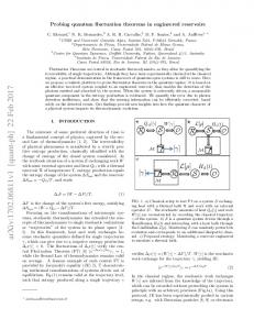
Figure 1

channel √ capacity of the classical binary symmetric channel with error probability (1 − 1 − ε2 )/2, C1 =

p p p p



 1 1 + 1 − ε2 log 1 + 1 − ε2 + 1 − 1 − ε2 log 1 − 1 − ε2 . 2

e we see that C1 < C e for 0 < ε < 1 (although the By comparing this quantity with C, difference between these functions is rather small: see Fig. 1, where the binary scale e it follows that strict superis used for quantities of information). Since C > C, additivity occurs: Cn > nC1 . However, it is a difficult problem to find practical block codes displaying this property in full measure (see [41]). The non-triviality of this problem can be effectively illustrated by the following simple example. By the entropy bound, the value C = log 2 is the absolute maximum of the channel capacity for all channels using states lying in two-dimensional unitary space. Moreover, this value is attained for a binary channel with orthogonal states, whereas for a binary channel with non-orthogonal states the inequality C < log 2 holds. Now let us consider a channel with three pure states given by vectors |ψ1 i, |ψ2 i, |ψ3 i such that hψi |ψj i = −1/2 for i 6= j. If we put πi = 1/3, then S π = 12 I, whence C = H(S π ) = log 2, in spite of the fact that the set of signal states contains none of the pairs of orthogonal states. The question is whether it is possible to find a constructive code approaching this theoretical bound? §4. Case of arbitrary states with bounded entropy The case of arbitrary signal states is much more complicated. In particular, efforts to find a correct generalization of the geometric bound (29) for pure states have so far been unsuccessful. Instead of this, the proof of the direct coding theorem for arbitrary states given in [26] and also in [42] is based on a generalization of the notion of the “jointly typical” sequences of classical information theory (see [8]).

1312

A. S. Holevo

This idea is realized by choosing the quantum decision rule in (25) as follows: Xwk =

X M

−1/2 P Pw l P

P Pw k P

l=1

X M

−1/2 P Pw l P

,

(44)

l=1

where P is the projection onto the typical subset of the operator X Sπ = πi Si , i∈A

and Pwk is the projection onto an appropriate modification of the typical subspace for the density operator Swk . Namely, for Pwk we choose the spectral projection of the operator Swk associated with eigenvalues λJ lying in the interval (e−n[H π (S( · ) )+δ] , en[H π (S( · ) )−δ] ). The main properties of the operator Pwk are as follows: Pw k

6 Sw

k

en[H π (S( · ) )+δ] ,

E Tr Swk (I − Pwk ) 6 .

(45) (46)


−1/2 P Pw l P in (44) is defined as a generalized
1/2 PM inverse of the operator Π = . We complete the definition of l=1 P Pw l P Π−1 by putting Π−1 = 0 on the null-space of Π which contains, in particular, the domain of the projection I − P . We denote by Pb the projection onto the domain PM of the operator l=1 P Pwl P . Then we have The operator Π−1 =

PM

l=1

P Pw l P

6 Pb 6 P,

l = 1, . . . , M.

(47)

In contrast to the original proof in [26] and [42], the proof given below leads straight to the purpose without recourse to spectral representations of the operators Swk .

Suppose that a c-q channel i → Si satis es the condition (24). Then its channel capacity is given by the expression

Theorem 3.

C = C ≡ sup ∆H(π).

(48)

π

Proof.

We restrict our attention to the case when the supremum is finite (the proof can easily be modified in the other case). Taking into account the results established in § II.3, it suffices to show that p(n, enR ) → 0

for R < C.

(49)

To simplify notation, in what follows we enumerate words only by the subscript w, omitting k.

Quantum coding theorems

1313

PM We put Aw = Pw P ( w0 =1 P Pw0 P )−1/2 and use the non-commutative analogue of the Cauchy–Bunyakovskii inequality | Tr Sw Aw |2

6 Tr Sw Aw ∗ Aw .

Then we have λ(W, X) 6

M M 1 X 2 X 2 [1 − | Tr Sw Aw | ] 6 [1 − Tr Sw Aw ], M w=1 M w=1


−1/2 PM 0 where Tr Sw Aw = Tr Sw Pw is a real number in the interval w 0 =1 P Pw P (0, 1). Further, using the inequality −2x−1/2 6 −3 + x,

x > 0,

which follows from (37), and taking into account (47) we obtain −2

X M

−1/2 P Pw 0 P

w 0 =1

6 −3P +

M X

P Pw 0 P

w 0 =1

6 −3P PwP +

M X

P Pw0 P,

w 0 =1

and therefore λ(W, X) 6

 M  M X 1 X 2 Tr Sw − 3 Tr Sw Pw P Pw P + Tr Sw Pw P Pw0 P M w=1 0 w =1

M 1 X = [2 Tr Sw (I − Pw P Pw P ) + M w=1

X

Tr Sw Pw P Pw0 P ].

w 0 : w 0 6=w

Using the estimate Tr Sw (I − Pw P Pw P ) = Tr Sw (I − Pw )P Pw P + Tr Sw (I − P )Pw − Tr Sw (I − P )Pw (I − P ) + Tr Sw (I − Pw )P + Tr Sw (I − P )

6 2[Tr Sw (I − Pw) + Tr Sw (I − P )], we arrive at the final inequality inf λ(W, X) 6 X

 M  X 1 X Tr P Sw P Pw0 . 4 Tr Sw (I − P ) + 4 Tr Sw (I − Pw ) + M w=1 0 0 w :w 6=w

(50) We now use the method of random coding, assuming again that the words w1 , . . . , wM are chosen in a random way and independently of each other but ⊗n with the same probability distribution (32). Then (cf. (33)) we have ESw = S π ,

1314

A. S. Holevo

P where S π = i πi Si . Averaging (50) and using the fact that the operators Sw and Pw0 are independent, we obtain E inf λ(W, X) 6 4 Tr S π (I − P ) + 4E Tr Sw (I − Pw ) + (M − 1) Tr S π P EPw0 . ⊗n

⊗n

X

Using inequalities (36) and (46), which express the generic character of the projections P and Pw , and properties of the operator trace, we have for n > n(π, , δ) E inf λ(W, X) 6 8 + (M − 1)kS π P k Tr EPw0 . ⊗n

X

By the property (35) of P , kS

⊗n

P k 6 e−n[H(S π )−δ] ,

and in view of the property (45) of Pw , Tr EPw0 = E Tr Pw0 Thus,

6 E Tr Sw

0

· en[H(S( · ) )+δ] = en[H(S( · ) )+δ] .

E inf λ(W, X) 6 8 + (M − 1) e−n[H(S π )−H(S( · ) )−2δ] . X

Let us choose the distribution π = π 0 in such a way that ∆H(π 0 ) > C − δ. Then for n > n(π 0 , , δ) (51) p(n, M ) 6 8 + (M − 1) e−n[C−3δ] . Thus, p(n, en[C−4δ] ) → 0 as n → ∞, whence (49) follows. IV. c-q channels with input constraints §1. Coding theorem The importance of the study of channels with input constraints was obvious even at the dawn of the age of quantum information theory. In particular, this study makes it possible to provide a mathematically correct formulation and answer to questions of the type: what is the maximum quantity of information that can be transmitted by a physical communication channel under limited energy resources? (See §§ 2, 3.) In this review, we restrict our attention to the case of c-q channels with classical input constraints. A channel with a discrete input alphabet A = {i} is our initial concern. Let f(i) be a non-negative function on the input alphabet. We consider the class 1 of distributions π on A that satisfy the condition X f(i)π(i) 6 E, (52)

P

i

where E is a positive number. We also assume that there is an additive restriction imposed on the input words w = (i1 , . . . , in ), f(i1 ) + · · · + f(in ) 6 nE,

(53)

Quantum coding theorems

and denote by

P

n

1315

the class of distributions on A satisfying the condition X

[f(i1 ) + · · · + f(in )]π(i1 , . . . , in ) 6 nE.

(54)

i1 ,...,in

Now we define quantities C, C as in § II.2, except that the supremum is taken only over distributions π of the class n , that is,

P

C = lim

n→∞

Cn , n

C = lim

n→∞

Cn , n

where Cn = sup sup In (π, X),

P

π∈

n

C n = sup ∆Hn (π),

P

X

π∈

n

and In (π, X) and ∆Hn (π) are analogues of the quantity (9) of information and the entropy bound (8), respectively, for tensor powers of the c-q channel in ⊗n under consideration. It must be emphasized that, as in the case of a channel without constraints, the sequence C n is additive, and therefore

H

C = sup ∆H(π).

P

π∈

(55)

1

Indeed, it suffices to verify that Cn

6 nC 1 .

(56)

The subadditivity of quantum entropy with respect to the tensor product implies that n X ∆H(π (k)), ∆Hn (π) 6 k=1

where π (k) is the kth marginal distribution of π on A. What is more, n X

∆H(π (k)) 6 n∆H(π),

k=1

Pn where π = n1 k=1 π (k), since ∆H(π) is an upward-convex function of π [19]. The inequality (54) can be written in the form 1 XX f(ik )π (k)(ik ) 6 E, n i n

k=1

whence it follows that π ∈ we obtain (56).

P

1

k

when π ∈

P

n.

Taking the supremum over π ∈

P

n,

1316

A. S. Holevo

Suppose that a c-q channel i → Si satis es the condition (24) and the input constraint (53). Then its channel capacity is given by the expression (55).

Theorem 4.

Proof.

It suffices to show that p(n, enR ) 6→ 0 if C < ∞ and R > C, and p(n, enR ) → 0 if condition (24) holds and R < C. The proof of the first statement (that is, the converse coding theorem) is based on the following modification of the inequality (23)
log M · 1 − p(n, M ) 6 sup sup In (π, X) + 1.

P

π∈

J

n

(57)

X

Indeed, as in the proof of Theorem 1, let denote a random variable describing values of the channel output when the decision rule X is used, and words of the code (W, X) are chosen in accordance with the distribution πM ascribing to each word the same probability 1/M . Let us use Fano’s inequality. Since the codewords satisfy condition (53), we have πM ∈ n , from which inequality (57) follows. Substituting M = enR, we arrive at the first statement of the theorem. In classical information theory, the direct coding theorem is proved by the use of random coding with the modified probability distribution (32) containing an additional multiplier that singles out only those words for which the constraint almost reduces to an equality [12], Ch. 7.3. A similiar method can be also used in the quantum case. Let π be a distribution satisfying condition (52), and P a probability measure on the set of tuples of M words relative to which Pnthe words are
independent and specified by the distribution (32). We put νn = P n1 k=1 f(ik ) 6 E and define a modified measure in such a way that words are independent as before, but the probability distribution is given by  n P
 νn−1πi1 · . . . · πin if f(ik ) 6 nE, e P w = (i1 , . . . , in ) = (58) k=1  0 otherwise.

P

P

e is the expectation corresponding to Note that Ef 6 E, since π ∈ 1 (here E (E) e the probability measure P (P)). By the central limit theorem, lim νn

n→∞

> 12 ,

e 6 2m Eξ for any non-negative random variable ξ depending on m words. whence Eξ As shown above, an upper bound of the error probability (25) is given by (50). We average this inequality with respect to P. Each summand in the right-hand side of (50) depends on no more than two different words and therefore e E inf λ(W, X) 6 4E inf λ(W, X). X

X

Moreover, for M = enR with R < C − 3δ, the expectation relative to P tends to e also tends to zero under the same zero as n → ∞. From this it follows that Eλ e condition. Since the measure P is concentrated on words satisfying condition (53),

Quantum coding theorems

1317

there is a sequence of codes of size M = enR such that the error probability λ(W, X) tends to zero as n → ∞. This result can be also generalized to the case of a continuous input alphabet A. Let A be a separable locally compact topological space. Suppose that a weakly continuous mapping x → Sx of A onto the set ( ) of density operators is given (weak continuity means the continuity of the matrix elements hψ| Sx |φi, ψ, φ ∈ ). It is sufficient for our purpose to restrict attention to the description of the corresponding c-q channel in terms of this mapping, although it is not difficult to construct a continuous analogue of the representation (17). The advantage of such a simplified description is that in this case the definition of the code can be formulated just as in the case of a discrete alphabet. Given an arbitrary Borel probability distribution π on A, we consider the quantity Z ∆H(π) = H(Sx ; S π ) π(dx), (59)

SH

H

A

Z

where Sπ =

Sx π(dx).

(60)

A

In view of the weak continuity of the function Sx , the last integral is well defined and gives a density operator in . Moreover, since the non-negative function H(Sx ; S π ) is lower semicontinuous [47], it follows that the integral (59) is likewise well defined. We consider the analogue of the condition (24),

H

sup H(Sx ) < ∞.

(61)

x∈A

Under this condition, the relation (8) holds with Z H(S( · ) ) = H(Sx ) π(dx). A

We also assume that a non-negative Borel function f is defined on A, and consider the set 1 of probability distributions π on A which satisfy the condition Z f(x) π(dx) 6 E. (62)

P

A

We introduce an additive constraint on the transmitted words by setting f(x1 ) + · · · + f(xn ) 6 E.

(63)

Proposition 2. Suppose that the mapping x → Sx is weakly continuous, the function f is lower semicontinuous, and the condition (61) holds. Then the channel capacity of a channel with input constraints (63) is given by the expression C = sup ∆H(π).

P

π∈

(64)

1

The proof of this statement, based on Theorem 4 and the continuity of quantum entropy, is given in an earlier version of this review [28].

1318

A. S. Holevo

§2. Gauss channel with one degree of freedom Quantum Gauss states are well defined for systems described by canonical commutation relations (one can find a simple introduction to this subject in [25], Ch. V). In this review, we restrict ourselves to gauge invariant states having an additional complex structure. In this case the canonical commutation relation for a system with one degree of freedom can be written in the form [a, a†] ⊆ I,

H

where a and a† are annihilation and creation operators, and is the space of an irreducible representation of this relation. Let the alphabet A be the entire complex plane C and let for each α ∈ C the density operator Sα be given by the relation 1 Sα = πN

Z

  |z − α|2 exp − |zihz| d2 z, N

(65)

where N is a positive number (the mean number of quanta) and |zi are vectors of coherent states, that is, eigenvectors of the annihilation operator (a|zi = z|zi), the set of which forms an overfilled system in . The first and second moments of the state Sα are given by the expressions

H

Tr Sα a = α,

Tr Sα a† a = N + |α|2 .

(66)

Recall also that Sα = V (α)S0 V (α)∗ , where the operators V (α) = exp(αa† − αa) are the unitary Weyl operators, and the spectral resolution of S0 takes the form S0 =

n ∞  1 X N |nihn|, N + 1 n=0 N + 1

(67)

where |ni are eigenvectors of the operator a† a of the number of quanta indexed by the corresponding eigenvalues n = 0, 1, . . . . In particular, the states (65) are of equal entropy, H(Sα ) = (N + 1) log(N + 1) − N log N ≡ g(N ),

(68)

where g(x) is a continuous concave monotone increasing function for x > 0. It is well known that the states Sα are of maximum entropy among all states satisfying (66). This suggests the following lemma.

Quantum coding theorems

Lemma 1. S satisfying

1319

The operator (67) is of maximum entropy among all density operators the condition Tr S a† a 6 N.

(69)

Proof.

We denote by S 0 the density operator that is diagonal in the basis {|ni} with diagonal elements sn = hn|S|ni. This operator satisfies (69) and the condition H(S 0 ) − H(S) = H(S; S 0 ) > 0.

This means that the maximum is attained for diagonal operators. Therefore, the P problem is to maximize H(S) = − s n n P log sn under the conditions sn > 0, P s = 1 and (69), which takes the form n n n nsn 6 N . Using Lagrange’s method, we obtain the solution (67). Since the operator (67) satisfies the conditions (66) (for α = 0), we see that it also is of maximum entropy among operators satisfying this condition. We now consider a c-q channel α → Sα that is a quantum analogue of a channel with additive Gauss noise (see [14], [16], and [22]). In this case condition (61) is trivially satisfied and, for any distribution π(d2 α) on the channel input, ∆H(π) = H(S π ) − H(S0 ), Z

where Sπ =

Sα π(d2 α).

We impose the additive constraint (63) on the input by setting f(α) = |α|2. Then the set 1 is defined by the relation Z |α|2 π(d2 α) 6 E. (70)

P

From a physical point of view the constant E is the “mean number of quanta” for the signal, which is proportional to the signal energy in the case of one degree of freedom. By virtue of (66), the constraint (70) implies that Tr S π a† a 6 N + E.

(71)

It follows from Lemma 1 that the maximum entropy H(S π ) = g(N + E) is attained for the Gaussian density operator   Z 1 |z|2 Sπ = exp − |zihz| d2 z, π(N + E) (N + E) which corresponds to the optimal probability distribution   1 |α|2 2 2 π(d α) = exp − d α. πE E

(72)

(73)

(74)

1320

A. S. Holevo

According to Proposition 2, the channel capacity is equal to C = C ≡ g(N + E) − g(N )       1 1 E = log 1 + + (N + E) log 1 + − N log 1 + . N +1 N +E N This expression was already proposed in [14] (see (4.28)) as a hypothetical upper bound on the amount of information transmitted by a quantum Gauss channel. On the other hand, it has been shown [13], [34] that this quantity is equal to the channel capacity of a quasiclassical “photon communication channel.” The reasoning above, based on Theorem 4 and Proposition 2, forms the first proof of the asymptotic equivalence (in the sense of channel capacity) of the Gauss c-q channel and this quasiclassical channel. For the sake of clarity, we give a description of the photon channel. We consider the discrete family of states Sm = P (m)S0 P (m)∗ ,

m = 0, 1, . . . ,

(75)

where P (m) is the energy shift operator defined by the relation P (m)|ni = |n + mi. Note that P (m) = P m , where P is an isometric operator conjugate to the phase operator [25]. All the states Sm are of equal entropy (68), coinciding with the entropy of the states Sα , and the mean number of quanta is equal to TR Sm a† a = N + m.

(76)

All the operators (75) are diagonal in the basis {|ni}, so that the channel m → Sm is quasiclassical. Imposing the constraint ∞ X m πm 6 E, (77) m=0

where πm is the input distribution, and introducing the density operator 0

Sπ =

∞ X

πm Sm ,

m=0

we see that, in view of (76), this operator satisfies the same condition (71). The maximum entropy, given by (72), is again attained again for the operator (73), whose spectral resolution has the form n ∞  X 1 N +E Sπ = |nihn|. (78) N + E + 1 n=0 N + E + 1 The maximum is attained by the following distribution [34]:   m  N E 1 N +E πm = δm0 + , N +E N +E N +E +1 N +E +1

m = 0, 1, . . . .

We consider the case of pure states when S0 = |0ih0|. Then the photon channel is determinate and admits error-free transmission. Its reliability function is equal to +∞. The corresponding Gauss channel uses non-orthogonal coherent states and a non-trivial reliability function (see [27]); nevertheless, it provides asymptotically error-free transmission at the same rate as the photon channel.

Quantum coding theorems

1321

§3. Classical signal on quantum background noise We now pass to the study of a more realistic dynamical model of the quantum Gauss channel. As in the classical case, we use the method of reducing a random process to a collection of parallel channels with one degree of freedom (see [12], § 8.3). In this case, such a reduction can be an additional tool for the quantization of the random process. It is possible to formulate our problem directly in terms of the quantum random process, but the evaluation of the channel capacity based on this formulation is an unsolved problem (see the discussion at the end of this section). We consider the periodic operator-valued function r X 2π~ωj
t ∈ [0, T ], (79) X(t) = aj e−iωj t +a†j eiωj t , T j where [0, T ] is the interval of observation, ωj =

2πj , T

j = 1, 2, . . . ,

(80)

is a collection of frequencies (depending on T ), and a†j and aj are the creation and annihilation operators describing the jth degree of freedom. In quantum electrodynamics, a similiar representation is used for the electric field component in a plane wave with periodic boundary conditions. To avoid problems connected with an infinite number of degrees of freedom, we restrict the range of summation in (79) to a finite set IT . In the case of a restricted range of frequencies, 0 < ω < ω < ω < ∞, we put IT = {j : ω 6 ωj 6 ω}. In the limiting case ω = 0 ω = ∞ we put IT = {j : ωT

6 ωj 6 ω T },

where ωT ↓ 0 and ωT ↑ ∞ as T → ∞. We emphasize that the corresponding energy operator satisfies the relation 1 4π

Z

T 2

X(t) dt =

X

0



~ω j

j

a†j aj

1 + 2

 .

(81)

We assume that the jth degree of freedom is described by the Gauss state (65), which we will denote by Sj (αj ), with first and second moments given by Tr Sj (αj )aj = αj ,

Tr Sj (αj )a†j aj = Nj + |αj |2 .

(82)

For a vector α = (αj ), we consider the state Sα =

O j

Sj (αj )

(83)

1322

A. S. Holevo

describing the process X(t), so that

Tr Sα

1 4π

Z

T

0

Tr Sα X(t) = α(t),   Z T X 1 1 2 X(t) dt = ~ωj Nj + + α(t)2 dt, 2 4π 0 j

(84)

where X

α(t) =

r

j

Z

1 4π


2π~ωj αj e−iωj t +αj eiωj t , T

T

α(t)2 dt =

X

0

~ωj |αj |2 .

(85) (86)

j

Thus, the signal is described by a real-valued function α(t). We impose the following restriction on the mean power of the signal: 1 4π

Z 0

T

α(t)2 dt 6 T E.

(87)

A code (W, X) is a collection (α1 ( · ), X1 ), . . . , (αM ( · ), XM ), where αk ( · ) are functions of the argument t ∈ [0, T ] representing different signal values. The channel capacity is defined as the supremum of the transmission rates R for which the infimum of the mean error probability λ(W, X) =

M 1 X (1 − Tr Sαj Xj ) M j=1

(88)

over all codes of size M = eT R tends to zero as T → ∞. From now on we shall use the notation (y)+ = max(y, 0). Theorem 5. Suppose that Nj = N (ωj ), where N (ω) is a continuous function. Then the channel capacity de ned above is equal to C=

1 2π

Z

ω

ω


g(Nθ (ω)) − g(N (ω)) + dω,

where Nθ (ω) =

1 , eθ~ω −1

ω > 0,

(89)

(90)

is the Planck distribution, and θ is a solution of the equation 1 2π

Z

ω

ω


~ω Nθ (ω) − N (ω) + dω = E.

(91)

Quantum coding theorems

1323

Proof.

We begin with the case when the frequency range is bounded and prove the inverse coding theorem: inf W,X λ(W, X) 6→ 0 for R > C. It follows from (57) and the entropy bound that   T R · 1 − inf λ(W, X) 6 CT + 1, W,X

(92)

where CT = sup ∆H(π) = sup [H(S π ) − H(S0 )], and the set

P

P

π∈ 1

P

π∈

1

1

of probability distributions is defined by the relation Z X



~ωj |αj |

2

π(d2 α) 6 ET.

(93)

j

Using Lemma 1, it is easy to see that one can restrict attention to Gauss distributions π. If we write Z ~ωj |αj |2 π(d2 αj ) = mj , then

X

CT = max

[g(Nj + mj ) − g(Nj )],

(94)

j∈IT

where the maximum is taken over the set mj

1 X ~ωj mj ∆ωj 2π

> 0,

6 E,

j∈IT

and ∆ωj =

2π . T

(95)

Defining the piecewise constant function NT (ω) = Nj , we have CT T where

M

6 2π1 Mmax (ω,ω)

Z

ωj−1 < ω < ωj ,



 g NT (ω) + m(ω) − g NT (ω) dω,

ω

ω

 (ω, ω) = m( · ) : m(ω) > 0;

1 2π

Z

ω

ω

 ~ωm(ω) dω 6 E .

Since the function N (ω) is uniformly continuous on [ω, ω], it follows that the family NT (ω) converges uniformly to N (ω) as T → ∞. Hence it follows that lim sup T →∞

CT T

1 6 Mmax (ω,ω) 2π

Z

ω

ω



 g N (ω) + m(ω) − g N (ω) dω.

1324

A. S. Holevo

Using the Kuhn–Tucker conditions, it is easy to show that the maximum is attained for
(96) m∗ (ω) = Nθ (ω) − N (ω) + and is equal to the quantity C defined by the relations (89)–(91). Therefore, in view of (92), we conclude that inf W,X λ(W, X) 6→ 0 for R > C. We now show that the mean error probability tends to zero when R < C. Let us consider the Gauss distribution  X  |αj |2 Y 2 π(d2 α) = exp − d αj , (97) m∗j j

where

j

m∗j = Nθ (ωj ) − Nj




(98)

+

and θ is chosen in such a way that 1 X ~ωj m∗j ∆ωj = E. 2π

(99)

j∈IT

(If m∗j = 0, then in (97) we have in mind a distribution degenerated at the point 0.) We now use the basic estimate (50) with word length n = 1 and replace δ by δT to conclude that inf λ(W, X) 6 X

 M  X 1 X Tr P Sαj P Pαk , 4 Tr Sαj (I − P ) + 4 Tr Sαj (I − Pαj ) + M j=1 k6=j

(100) where P is the spectral projection of the operator S π associated with the interval (e−[H(S π )+δT ] , e−[H(S π )−δT ] ), and Pα is the spectral projection of the operator Sα associated with the interval (e−[H(S( · ) )+δT ] , e−[H(S( · ) )−δT ] ). Since the density operators Sα are unitarily equivalent to S0 , it follows that H(S( · ) ) = H(S0 ), and the second term in the right-hand side of (100) is equal to

We have

Tr S0 (I − P0 ).

(101)

 Tr S0 (I − P0 ) = Pr | − log λ( · ) − H(S0 )| > δT ,

(102)

where Pr denotes a distribution specified by the eigenvalues λ( · ) of the density operator S0 . By Chebyshev’s inequality, this probability does not exceed D(log λ( · ) )/δ 2 T 2 . On the other hand, D(log λ( · ) ) =

X j

Dj (log λ( · ) ),

Quantum coding theorems

1325

where Dj is variance of the random variable log λ( · ) for the jth degree of freedom. It follows from (67) that the eigenvalues of the operator Sj (0) are λjn =

Njn ; (Nj + 1)n+1

n = 0, 1, . . .,

whence Dj (log λ( · ) ) =

∞ X


2 − log λjn − H(S0 ) λjn

(103)

n=0

= log2

∞ Njn Nj + 1 X (n − Nj )2 = F (Nj ), Nj n=0 (Nj + 1)n+1

where the function F (x) = x(x + 1) log2 is bounded on (0, ∞). The net result is that P Tr S0 (I − P0 ) 6

j

x+1 x

F (Nj )

δ2T 2

(104)

.

(105)

Note that a similiar bound holds for Tr S π (I − P ) with Nj replaced by Nj + m∗j . We now consider the case when the words α1 , . . . , αM are chosen at random with e that is defined similiarly to (58) starting from a distribution P a joint distribution P relative to which the words are independent and have the identical distribution π(d2 α). Then e Eξ 6 2m Eξ for any non-negative random variable ξ depending on m words. Therefore, it follows from (100) that e inf λ(W, X) E X

6 M1

 M  X X 4E Tr P Sα(j) P Pα(k) 8E Tr Sα(j) (I − P ) + 4 Tr S0 (I − P0 ) + j=1

k6=j −[∆H(π)−2δT ]

= 8 Tr S π (I − P ) + 4 Tr S0 (I − P0 ) + 4(M − 1) e P P 8 j∈IT F (Nj + m∗j ) 4 j∈IT F (Nj ) 6 + + 4(M − 1) e−[CT −2δT ] . δ2 T 2 δ2T 2 Since the function F (x) is bounded and the number of elements in IT is proportional to T , it follows that the sums in the numerators are of order T , and the first two terms are of order T −1 . To complete the proof, it remains to show that lim inf T →∞

CT T

> C.

(106)

Suppose that the function m∗ (ω) is specified by (96) and ωj0 is a point in [ωj−1, ωj ] at which this function reaches a minimum. Then Z ω 1 X 1 ~ωj0 m∗ (ωj0 ) 6 ~ωm∗ (ω) dω = E, 2π 2π ω j∈IT

1326

A. S. Holevo

whence it follows that CT T

> 2π1

X
 g N (ωj ) + m∗ (ωj0 ) − g(N (ωj )) ∆ωj . j∈IT

Since the functions N (ω) and m∗ (ω) are continuous, the sums in the right-hand side tend to Z ω

  g N (ω) + m∗ (ω) − g N (ω) dω = C. ω

This completes the proof. We now consider the case when the frequency range (0, ∞) is unbounded. Arguing as above, we see that it suffices to establish the relation Z ∞ 

 CT 1 lim = C(0, ∞) ≡ max g N (ω) + m(ω) − g N (ω) dω, (107) T →∞ T M(0,∞) 2π 0 where

M(0, ∞) =

 m( · ) : m(ω)

> 0,

1 2π

Z

∞

~ωm(ω)dω

0

6E

 .

(108)

The maximum is attained by a function m∗ (ω) of the form (96), where θ is chosen in such a way that Z ∞ 1 ~ωm∗ (ω) dω = E. 2π 0 Let us choose numbers 0 < ω < ω < ∞. Omitting frequencies outside this interval, we obtain lim inf T →∞

CT T

1 > Mmax (ω,ω) 2π

> 2π1

Z

Z

ω



 g N (ω) + m(ω) − g N (ω) dω

ω



 g N (ω) + m∗ (ω) − g N (ω) dω,

ω

ω

M

since m∗ ( · ) ∈ (ω, ω). Passing to the limit as ω → 0, ω → ∞, this proves that holds in relation (107). For the reverse inequality, we consider the relation CT 1 X = [g(Nj + m∗j ) − g(Nj )]∆ωj , T 2π j where m∗j =



1 eθT ~ωj −1

>

(109)

 − Nj +

and θT is chosen in such a way that 1 X ~ωj m∗j ∆ωj = E. 2π j

(110)

Quantum coding theorems

1327

Introducing the piecewise constant functions NT (ω) = Nj ,

mT (ω) = m∗j

for ωj−1 < ω 6 ωj ,

we see that the right-hand side of (109) becomes Z ∞

  1 g NT (ω) + mT (ω) − g NT (ω) dω 2π 0 Z ∞ 

 1 = g N (ω) + mT (ω) − g N (ω) dω 2π 0 Z ∞ 



 1 g NT (ω) + mT (ω) − g N (ω) + mT (ω) +g N (ω) −g NT (ω) dω. + 2π 0 Taking into account the inequality Z ∞ 1 ~ωmT (ω) dω 2π 0

1 6 2π

X

~ωj m∗j ∆ωj = E,

j

we conclude that the first term is less than or equal to Z ∞ 

 1 max g N (ω) + m(ω) − g N (ω) dω = C(0, ∞). M(0,∞) 2π 0 It remains to show that the second term tends to zero. This fact follows from Lebesgue’s theorem on dominated convergence. Since N (ω) is continuous, it follows that NT (ω) → N (ω) and g(NT (ω)) → g(N (ω)) pointwise. Furthermore, notice that the θT are separated from zero as T → ∞. Indeed, if θT ↓ 0 for some sequence T → ∞, then the corresponding sequence of continuous functions   1 − N (ω) eθT ~ω −1 + tends to ∞ uniformly on any interval 0 < ω 6 ω 6 ω < ∞, contradicting (110). Hence, for any ω > 0 the quantities   1 N (ω) + mT (ω) = max θT ~ω , N (ω) e −1 remain bounded as T → ∞. Since the function g(ω) is uniformly continuous on any interval, we have

g NT (ω) + mT (ω) − g N (ω) + mT (ω) → 0. It remains to show that the terms of the integrand are bounded above by an integrable function. In view of the fact that h00 (x) 6 0 for x > 0, we see that g(x + y) − g(x) 6 g(y) for x, y > 0. Therefore, a term of the integrand is bounded above by the function 2g(mT (ω)). We have mT (ω) 6

1 eθT ~ω

1 6 . θ ~ −1 e ω −1 0

1328

A. S. Holevo

Thus, g(mT (ω))

6g





1

=

eθ0 ~ω −1

θ0 ~ω − log(1 − e−θ0 ~ω ), eθ0 ~ω −1

where the right-hand side is a positive integrable function. The formulae for channel capacity are of especially simple form in the case of equilibrium noise N (ω) = NθP (ω) ≡ (eθP ~ω −1)−1 , where θP is specified by the equation Z ∞ 1 ~ω dω = P. θ P 2π 0 e ~ω −1 Using the formula

we have θP = 1 2π

Z 0

∞

p

Z

∞

ex

0

x π2 dx = , −1 6

π/(12~P ), and


1 g NθP (ω) dω = 2π

∞

Z 0

r  πP θP ~ω −θP ~ω ) dω = . − log(1 − e θ ~ ω P e −1 3~ (111)

From this it follows that 1 C(0, ∞) = 2π

Z

∞



 g NθP +E (ω) − g NθP (ω) dω =

r

0

π(P + E) − 3~

r

πP , (112) 3~

and this quantity coincides with the channel capacity of a photon channel with unbounded frequency range, and this was calculated in [34]. We now try to formulate the problem in terms of a limit random process. We expect that in the limit as T → ∞ the periodic process (79) becomes X(t) = α(t) + Y (t),

t > 0,

where α(t) is a classical signal and Y (t) is the quantum Gauss noise Z

√
~ω dAω e−iωt +dA†ω eiωt .

∞

Y (t) =

(113)

0

Here Aω , ω that

> 0, is a quantum Gauss process with independent increments such [dAω , dA†λ] = δ(ω − λ) dω dλ,

the average is equal to zero, and the correlation function is given by hdA†ω dAλi = δ(ω − λ)N (ω) dω dλ. It follows from (113) that Z [Y (t), Y (s)] = 2i~ 0

∞

ω sin ω(s − t) dω = 2i~πδ 0 (t − s)

(114)

Quantum coding theorems

1329

and the quantum noise correlation function is hY (t)Y (s)i = B(t − s) + K(t − s), Z

where B(t) = 2~

(115)

∞

ωN (ω) cos ωt dω 0

and the function Z

∞

K(t) = ~

ω e−iωt dω = −~[t−2 − iπδ 0 (t)]

0

is the correlation function of vacuum noise (corresponding to zero temperature). The process X(t) is observed in the time interval [0, T ]. This means that Gauss (quasi-free) states with average α(t) and correlation function (115) are considered on the C ∗ -algebra of canonical commutation relations generated by the operators X(t), t ∈ [0, T ], and specified by (114) (see, for example, [21]). Under the condition (87) on the signal power, the channel capacity is defined as above, preceding Theorem 5. The proof of Theorem 5 makes plausible the statement that the capacity of such a channel is given by (112). However, the classical method of proof by reduction to parallel channels with one degree of freedom [12] meets with new difficulties here. First, in the new case the kernels (114) and (115) are already distributions. A more telling circumstance is that, in the classical case, there are only two quadratic forms, defined by the correlation function and the energy constraint (the second form is simply the scalar product in L2 ), and these can be diagonalized simultaneously by solving the integral equation with kernel (115). In the quantum case, a skew-symmetric form defined by the commutator is also present. To obtain an expansion in independent quantum degrees of freedom, this form also must be transformed into canonical form. However, there is no way of doing this for finite T , in spite of the fact that it occurs (as is shown in the proof of Theorem 5) when T → ∞. Bibliography [1] [2]

[3]

[4] [5] [6] [7] [8]

H. Barnum, E. Knill, and M. A. Nielsen, “On quantum fidelities and channel capacities”, LANL Report no. QP9809010, Los Alamos 1998. H. Barnum, M. A. Nielsen, and B. Schumacher, “Information transmission through noisy quantum channels”, LANL Report no. QP9702049, Los Alamos 1997; see also Phys. Rev. A 57 (1998), 4153–4175. C. H. Bennett, C. A. Fuchs, and J. A. Smolin, “Entanglement-enhanced classical communication on a noisy quantum channel”, in: Quantum Communication, Computing and Measurement, Plenum, New York 1997, pp. 79–88. C. H. Bennett, “Classical and quantum information transmission and interactions”, in: Quantum Communication, Computing and Measurement, Plenum, New York 1997, pp. 25–39. M. V. Burnashev and A. S. Holevo, “On reliability function of quantum communication channel”, LANL Report no. QP9703013, Los Alamos 1997. (Russian) A. R. Calderbank and P. W. Shor, “Good quantum error-correcting codes exist”, Phys. Rev. A 54 (1996), 1098–1105. C. M. Caves and P. B. Drummond, “Quantum limits of bosonic communication rates”, Rev. Modern Phys. 66 (1994), 481–538. T. M. Cover and J. A. Thomas, Elements of Information Theory, Wiley, New York 1991.

1330 [9] [10] [11] [12] [13] [14]

[15] [16] [17] [18]

[19]

[20]

[21] [22] [23]

[24]

[25] [26]

[27] [28] [29] [30]

[31] [32]

A. S. Holevo M. Echigo and M. Nakamura, “A remark on the concept of channels”, Proc. Japan Acad. 38:5 (1962), 307–309. G. D. Forney, Jr., MS thesis, MIT, Cambridge, MA 1963. A. Fujivara and H. Nagaoka, “Operational capacity and semi-classicality of quantum channels”, IEEE Trans. Inform. Theory. 44 (1998), 1071–1086. R. G. Gallagher, Information theory and reliable communications, Wiley, New York 1968; Russian transl., Sov. Radio, Moscow 1974. J. P. Gordon, “Quantum effects in communication systems”, Proc. IRE 50 (1962), 1898–1908. J. P. Gordon, “Noise at optical frequencies; information theory”, in: Quantum Electronics and Coherent Light, Proc. Internat. School of Phys. “Enrico Fermi”, course 31, Academic Press, New York 1964, pp. 156–181. P. Hausladen, R. Jozsa, B. Schumacher, M. Westmoreland, and W. Wootters, “Classical information capacity of a quantum channel”, Phys. Rev. A 54 (1996), 1869–1876. C. W. Helstrom, Quantum hypotheses testing and estimation theory, Academic Press, New York 1976; Russian transl., Mir, Moscow 1978. A. Ya. Khinchin, “On the fundamental theorems of information theory”, Uspekhi Mat. Nauk 11:1 (1956), 17–75. (Russian) A. S. Holevo, “On the mathematical theory of quantum communication channels”, Problemy Peredachi Informatsii 8:1 (1972), 62–71; English transl., Problems Inform. Transmission 8 (1972), 47–56. A. S. Holevo, “Some estimates for the amount of information transmittable by a quantum communications channel”, Problemy Peredachi Informatsii 9:3 (1973), 3–11; English transl., Problems Inform. Transmission 9 (1973), 177–183. A. S. Holevo, “Remarks on optimal quantum measurements”, Problemy Peredachi Informatsii 10:4 (1974), 51–55; English transl. in Problems Inform. Transmission 10 (1974). A. S. Holevo, “Investigations in the general theory of statistical decisions”, Trudy Mat. Inst. Steklov. 124 (1976); English transl. in Proc. Steklov Inst. Math. 124 (1978). A. S. Holevo, “Problems in the mathematical theory of quantum communication channels”, Rep. Math. Phys. 12:2 (1977), 273–278. A. S. Holevo, “Asymptotically optimal hypothesis-testing in quantum statistics”, Teor. Veroyatnost. i Primenen. 23 (1978), 429–432; English transl. in Theory Probab. Appl. 23 (1956). A. S. Holevo, “On channel capacity of a quantum communication channel”, Problemy Peredachi Informatsii. 15:4 (1979), 3–11; English transl., Problems Inform. Transmission 15 (1979), 247–253. A. S. Holevo, Probabilistic and statistical aspects of quantum theory, Nauka, Moscow 1980; English transl., North-Holland, Amsterdam-New York 1982. A. S. Holevo, “The capacity of quantum communication channel with general signal states”, LANL Report no. QP9611023, Los Alamos 1996; see also IEEE Trans. Inform. Theory 44:1 (1998), 269–272. A. S. Holevo, “On quantum communication channels with constrained inputs”, LANL Report no. QP9705054, Los Alamos 1997. A. S. Holevo, “Coding theorems for quantum channels”, Tamagawa Univ. Research Review 1998, no. 4. R. Jozsa and B. Schumacher, “A new proof of the quantum noiseless coding theorem”, J. Modern Optics 41 (1994), 2343–2349. K. Kato, M. Osaki, T. Suzuki, M. Ban, and O. Hirota, “Upper bound of the accessible information and lower bound of the Bayes cost in quantum signal detection processes”, in: Quantum Communication, Computing and Measurement, Plenum, New York 1997, pp. 63–71. A. Kossakowski, Talk at the symposium on quantum probability and applications, Gda´ nsk 1997 (unpublished). K. Kraus, States, eects and operations. Fundamental notions of quantum theory, Lecture Notes in Physics, vol. 90, Springer-Verlag, Berlin 1983.

Quantum coding theorems

1331

[33] M. G. Krein, “On Bari bases of a Hilbert space”, Uspekhi Mat. Nauk 12:3 (1957), 333–341. (Russian) [34] D. S. Lebedev and L. B. Levitin, “The maximum amount of information transmissible by an electromagnetic field”, Dokl. Akad. Nauk SSSR 149 (1963), 1299–1302; English transl., Soviet Physics Dokl. 8 (1963), 377–379. [35] L. B. Levitin, “On quantum measure of information”, in: Proc. IV All-Union Conference on Information Transmission and Coding Theory, Tashkent, 1969, pp. 111–115. (Russian) [36] L. B. Levitin, “Optimal quantum measurement for two pure and mixed states”, in: Quantum Communications and Measurement, Plenum, New York 1995, pp. 439–448. [37] E. H. Lieb and M. B. Ruskai, “Proof of the strong subadditivity of quantum mechanical entropy”, J. Math. Phys. 14 (1973), 1938–1941. [38] G. Lindblad, “Entropy, information and quantum measurements”, Commun. Math. Phys. 33 (1973), 305–322; “Expectations and entropy inequalities for finite quantum systems” ibid 39 (1974), 111–119; “Completely positive maps and entropy inequalities” ibid 40 (1975), 147–151. [39] M. A. Naimark, “Spectral functions of symmetric operator”, Izv. Akad. Nauk SSSR Ser. Mat. 4 (1940), 277–318. (Russian) [40] M. Ohya and D. Petz, Quantum entropy and its use, Springer-Verlag, Berlin 1993. [41] M. Sasaki, K. Kato, M. Izutsu, and O. Hirota, Quantum channels showing superadditivity in the capacity, Preprint, Tamagawa Univ. 1997. [42] B. Schumacher and M. D. Westmoreland, “Sending classical information via noisy quantum channels”, Phys. Rev. A 56:1 (1997), 131–138. [43] A. Steane, “Quantum computing”, LANL Report no. QP9708022, Los Alamos 1997. [44] W. F. Stinespring, “Positive functions on C ∗ -algebras”, Proc. Amer. Math. Soc. 6 (1955), 211–216. [45] R. L. Stratonovich and A. G. Vantsyan, “Asymptotically error-free decoding in pure quantum channels”, Probl. Control Inform. Theory 7:3 (1978), 161–174. [46] A. Uhlmann, “Relative entropy and the Wigner–Yanase–Dyson–Lieb concavity in an interpolation theory”, Comm. Math. Phys. 54 (1977), 21–32. [47] A. Wehrl, “General properties of entropy”, Rev. Modern Phys. 50:2 (1978), 221–260. [48] H. P. Yuen and M. Ozawa, “Ultimate information carrying limit of quantum systems”, Phys. Rev. Lett. 70:4 (1993), 363–366. Steklov Mathematical Institute Received 23/JAN/98

Typeset by AMS-TEX