Quantum computing with electrical circuits - UGA Physics - University ...

Quantum computing with electrical circuits: Hamiltonian construction for basic qubit-resonator models Michael R. Geller Department of Physics and Astronomy, University of Georgia, Athens, Georgia 30602, USA June 4, 2007 Abstract Recent experiments motivated by applications to quantum information processing are probing a new and fascinating regime of electrical engineering—that of quantum electrical circuits—where macroscopic collective variables such as polarization charge and electric current exhibit quantum coherence. Here I discuss the problem of constructing a quantum mechanical Hamiltonian for the low-frequency modes of such a circuit, focusing on the case of a superconducting qubit coupled to a harmonic oscillator or resonator, an architecture that is being pursued by several experimental groups.

1

Quantum gate design

In the quantum circuit model of quantum information processing, an arbitrary unitary transformation on N qubits can be decomposed into a sequence of certain universal two-qubit logical operations acting on pairs of qubits, combined with arbitrary single-qubit rotations [1]. The purpose of quantum gate design is to develop experimental protocols or “machine language code” to implement these elementary operations. For quantum information processing architectures based on superconducting circuits [2, 3], the first step is to construct an effective Hamiltonian for the system. Whereas the fully microscopic Hamiltonian for the electronic and ionic degrees of freedom in the conductors forming the circuit is known, at least in principle, the Hamiltonian of interest here describes only the relevant low-energy modes of that circuit. A rigorous construction might involve making a canonical transformation from the microscopic quantum degrees of freedom to a set of collective modes. Here I follow a simpler and more intuitive phenomenological quantization method, whereby a classical description based on Kirkoff’s laws is derived first, and then later canonically quantized. It is important to realize that such an approach is not based on first principles and must be confirmed experimentally.

2

The phase qubit

The primitive building block for any superconducting qubit is the Josephson junction (JJ) shown in Fig. 1. The low-energy dynamics of this system is governed by the phase difference ϕ between the condensate wave functions or order parameters on the two sides of the insulating barrier. The phase difference is an operator canonically conjugate to the Cooper-pair number difference N, according to1 [ϕ, N] = i.

(1)

The low-energy eigenstates ψm (ϕ) of the JJ can be regarded as probability-amplitude distributions in ϕ. As will be explained below, the potential energy U(ϕ) of the JJ is manipulated by applying a bias current I to the junction, providing an external control of the quantum 1 We

∂ define the momentum P to be canonically conjugate to ϕ, and N ≡ P/¯ h. In the phase representation, N = −i ∂ϕ .

1

V=a dj/dt I

I

=

I0

C

Figure 1: Circuit model for a current-biased JJ, neglecting dissipation. Here α ≡ ¯h/2e.

states ψm (ϕ), including the qubit energy-level spacing ǫ. The crossed box in Fig. 1 represents a “real” JJ. The cross alone represents a nonlinear element that satisfies the Josephson equations2 I = I0 sin ϕ

and

V = αϕ, ˙

(2)

with critical current I0 . The capacitor accounts for junction charging.3 A single JJ is characterized by two energy scales, the Josephson coupling energy EJ ≡

h ¯ I0 , 2e

(3)

where e is the magnitude of the electron charge, and the Cooper-pair charging energy (2e)2 , 2C

Ec ≡

(4)

with C the junction capacitance. For example, EJ = 2.05 meV×I0 [µA]

and

Ec =

320 neV , C[pF]

(5)

where I0 [µA] and C[pF] are the critical current and junction capacitance in microamperes and picofarads, respectively. In the regimes of interest to quantum computation, EJ and Ec are assumed to be larger than the thermal energy kB T but smaller than the superconducting energy gap ∆sc , which is about 180 µeV in Al. The relative size of EJ and Ec vary, depending on the specific qubit implementation. The basic phase qubit considered here consists of a JJ with an external current bias, and is shown in Fig. 2. The classical Lagrangian for this circuit is 1 LJJ = M ϕ˙ 2 − U, 2

M≡

h ¯2 . 2Ec

Here

2α


U ≡ −EJ cos ϕ + s ϕ ,

with

s≡

(6) I , I0

(7)

≡¯ h/2e. provides a simple mean-field treatment of the inter-condensate electron-electron interaction neglected in the standard tunneling Hamiltonian formalism on which the Josephson equations are based. 3 This

2

j

I

Figure 2: Basic phase qubit circuit.

3 2

U/EJ

1 0 -1 -2 -3

-10

0

10

ϕ (radians) Figure 3: Effective potential for a current-biased JJ. The slope of the cosine potential is s. The potential is harmonic for the qubit states unless s is very close to 1.

is the effective potential energy of the JJ, shown in Fig. 3. Note that the “mass” M in (6) actually has dimensions of mass × length2. The form (6) results from equating the sum of the currents flowing through the capacitor and ideal Josephson element to I. The phase qubit implementation uses EJ ≫ Ec . According to the Josephson equations, the classical canonical momentum P = ∂L is pro∂ ϕ˙ portional to the charge Q or to the number of Cooper pairs Q/2e on the capacitor according to P = h ¯ Q/2e. The quantum Hamiltonian can then be written as HJJ = Ec N 2 + U,

(8)

where ϕ and N are operators satisfying (1). Because U depends on s, which itself depends on time, HJJ is generally time-dependent. The low lying stationary states when s < 1 are shown in Fig. 4. The two lowest eigenstates |0i and |1i are used to make a qubit. ǫ is the level spacing and ∆U is the height of the barrier. A useful “spin 21 ” form of the phase qubit Hamiltonian follows by projecting (8) to the qubit subspace. There are two natural ways of doing this. The first is to use the basis of the

3

Figure 4: Effective potential in the anharmonic regime, with s very close to 1. State preparation and readout are carried out in this regime.

s-dependent eigenstates, in which case H=−

h ¯ ωp z σ , 2

(9)

where 1

ωp ≡ ωp0 (1 − s2 ) 4

and

ωp0 ≡

p

2Ec EJ /¯ h.

(10)

The s-dependent eigenstates are called instantaneous eigenstates, because s is usually changing with time. The time-dependent Schr¨odinger equation in this basis contains additional terms coming from the time-dependence of the basis states themselves, which can be calculated in closed form in the harmonic limit [4]. These additional terms account for all nonadiabatic effects. The second spin form uses a basis of eigenstates with a fixed value of bias, s0 . In this case H=−

h ¯ ωp (s0 ) z EJ ℓ σ − √ (s − s0 ) σ x , 2 2

(11)

where ℓ ≡ ℓ0 (1 − s0 )

− 81

and

ℓ0 ≡



2Ec EJ

 41

.

(12)

This form is restricted to |s − s0 | ≪ 1, but it is very useful for describing rf pulses. The angle ℓ characterizes the width of the eigenstates in ϕ. For example, in the s0 eigenstate basis (and with s0 in the harmonic regime), we have ϕ = ϕ01 σ x + arcsin(s0 ) I,

with

ϕmm′ ≡ hm|ϕ|m′ i.

(13)

Here √ ϕmm′ is an effective dipole moment (with dimensions of angle, not length), and ϕ01 = ℓ/ 2. 4

i

n

t

i

n

t

o



s

c

x

o

s

c

o

s

c

Figure 5: Circuit model for a superconducting qubit coupled to a parallel LC oscillator.

3

Qubit-oscillator models

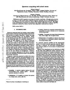
Circuit diagrams for an rf squid capacitively coupled to parallel and series LC oscillators are shown in Figs. 5 and 6. Φx is an external flux bias, and ϕ is the phase difference across the JJ (the phase of the ungrounded superconductor relative to the grounded side is ϕ). Quantization of the total magnetic flux Φ in the squid loop leads to the condition (in cgs units) ϕ hc Φ = Φx − cLI = Φsc , Φsc ≡ (14) 2π 2e where I is the current flowing downward through the Josephson junction, related to ϕ by αC ϕ¨ + I0 sin ϕ = I.

(15)

Here C and I0 are the usual JJ capacitance and critical-current parameters, and α≡

h ¯ . 2e

(16)

The minus sign in (14) reflects the diamagnetic (for 0 < ϕ < π) screening by the superconducting loop. The quantization condition (14) assumes an isolated squid (specifically, that no current is being provided by the coupling capacitor). In Figs. 5 and 6 the voltage across the JJ is V = αϕ. ˙ (17) 3.1

JJ coupled to parallel LC oscillator

Referring to Fig. 5, the equations of motion for ϕ and q are α2 (C + Cint )ϕ¨ + EJ sin ϕ +

αΦsc αΦext Cint ϕ− =α q˙ 2πcL cL Cosc

(18)

and   ... q Cint q¨ + = αLosc Cint ϕ . Losc 1 + Cosc Cosc 5

(19)

i

n

t

o



s

c

x

o

s

c

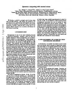
Figure 6: Circuit model for qubit coupled to series LC oscillator. m

Surprisingly, it is not possible to find a Lagrangian (local in time and a polynomial in ddtmϕ n and ddtnq ) that gives these equations of motion. To proceed, we make a transformation from q to a dimensionless node-flux variable φ, defined as Z t 1 q(t′ ) dt′ , (20) φ(t) ≡ αCosc −∞ ˙ and integrate the equation resulting from (19) over time. This leads to the use q = αCosc φ, coupled equations α2 (C + Cint )ϕ¨ + EJ sin ϕ +

α2 2πα2 x ϕ− = α2 Cint φ¨ L L

(21)

and α2 α2 (Cosc + Cint )φ¨ + φ = α2 Cint ϕ¨ + const, Losc

(22)

where

Φx (23) Φsc is the dimensionless flux bias. The integration constant in (22) acts as an applied static force and can be dropped (corresponding to a shift in φ). Note the symmetry in the cross-coupling terms on the right-hand-sides of (21) and (22). A Lagrangian leading to (21) and (22) is x≡

L=


2 α2 Cosc 2 α2 2 α2 C 2 α2 ˙ ϕ − 2πx + φ˙ − ϕ˙ + EJ cos ϕ − φ − α2 Cint ϕ˙ φ. 2 2L 2 2Losc

(24)

The simple capacitance renormalizations C → C +Cint and Cosc → Cosc +Cint present in (21) and (22) have been ignored here but can easily be accounted for below. The velocity-velocity y coupling in (24) will lead to a σJy σosc interaction term in the Hamiltonian. The canonical momenta are pϕ = α2 C ϕ˙ − α2 Cint φ˙

and 6

pφ = α2 Cosc φ˙ − α2 Cint ϕ. ˙

(25)

The velocities in terms of these momenta are ϕ˙ =

Cosc pϕ + Cint pφ 2 α2 (CCosc − Cint )

and

Cint pϕ + C pφ φ˙ = 2 . 2 α (CCosc − Cint )

(26)

Quantization then leads to H = pϕ ϕ˙ + pφ φ˙ − L = Hϕ + Hφ + δH,

(27)

where [ϕ, pϕ ] = i¯ h, [φ, pφ ] = i¯ h, and δH = Typically Cint ≪

Cint pϕ pφ . 2 α2 (CCosc − Cint )

(28)

√ 2 CCosc , allowing the Cint in the denominator to be dropped. Furthermore, Hϕ = Ec N 2 − EJ cos ϕ +

and


2 α2 ϕ − 2πx 2L

(29)

p2φ α 2 φ2 + . (30) 2α2 Cosc 2Losc The kinetic energy in Hφ is electrical in origin and the potential energy is magnetic. The strength of quantum fluctuations is characterized by the dimensionless quantity r h ¯ . (31) ℓφ ≡ 2 α Cosc ωosc Hφ =

Finally, I simplify (28) by projecting the squid and oscillator into their {|0i, |1i} subspaces. Then h ¯ ϕ01 ǫ y pϕ → σ , (32) 2Ec where ϕ01 ≡ h0|ϕ|1i is the JJ dipole moment and ǫ ≡ ǫ1 − ǫ0 is the qubit level spacing (both calculated in the absence of coupling to the oscillator). To obtain this result I have used the identity [ϕ, Hϕ ] = 2iEc N, allowing us to relate momentum and dipole matrix elements. The oscillator momentum operator projects similarly, pφ → √

h ¯ σy , 2 ℓφ

(33)

2 Then we obtain [dropping the Cint in the denominator of (28)] y δH = gσJy σosc ,

(parallel circuit)

where

(34)

  √  2 ϕ01 1 Cint h ¯ 2 Cint ϕ01 ǫ ǫ. (35) = g= √ 2 Cosc ℓφ 2 2 α2 CCosc Ec ℓφ √ Note that in the harmonic junction limit, ϕ01 = ℓϕ / 2, with ℓϕ the width of the wave functions in the junction.

7

3.2

JJ coupled to series LC oscillator

Referring to Fig. 6, the equations of motion are α2 C ϕ¨ + EJ sin ϕ + and, assuming Cint 6= 0, Losc q¨ +

2πα2 x α2 ϕ− = −αq˙ L L

(36)

q = αϕ, ˙ ′ Cosc

(37)

−1 −1 ′ −1 where Cosc ≡ (Cosc +Cint ) . Note that the capacitance Cint does not enter the cross-coupling terms on the right-hand-sides of (36) and (37). This is an indication that the qubit-oscillator coupling in this system is nonperturbative: The limit Cint → 0 differs from the case Cint = 0, and there is no small parameter associated with the interaction. A Lagrangian leading to (36) and (37) is4

L=


2 Losc 2 α2 C 2 α2 1 2 q + α ϕq. ˙ ϕ − 2πx + ϕ˙ + EJ cos ϕ − q˙ − ′ 2 2L 2 2Cosc

(38)

The canonical momenta are

pϕ = α2 C ϕ˙ + αq

and

pq = Losc q, ˙

(39)

leading to the quantum Hamiltonian H=


2 p2q (pϕ − αq)2 α2 q2 . ϕ − 2πx − E cos ϕ + + + J ′ 2α2 C 2L 2Losc 2Cosc

(40)

The squid sees the oscillator as a source of vector potential A ∝ αq, whose time derivative describes an effective electric field. Noting that the “diamagnetic” A2 term serves to further decrease the oscillator capacitance, I obtain H = Hϕ + Hq + δH,

(41)

where Hq is the oscillator Hamiltonian

where and


p2q q2 † 1 = h ¯ ω a a + + Hq = , osc 2 ′ 2Losc 2Cosc ′ −1 −1 Cosc ≡ Cosc + C −1 + Cint

δH = −

pϕ q αC

ωosc ≡
−1

,

s

1 , ′ Losc Cosc

(42)

(43) (44)

is the qubit-oscillator interaction. In the {|0i, |1i} subspace of the series oscillator, ℓq q → √ σx, 2 4 An

alternative form for L has an interaction term δL = −α ϕq. ˙

8

(45)

i

n

t

i



x

n

t



x

2 1

2

2 1

1

Figure 7: Capacitively coupled qubits.

where ℓq ≡ Then we have

r

h ¯ . Losc ωosc

x δH = −gσJy σosc ,

where

(series circuit)

(46) (47)

ϕ01 ℓq (48) g = √ ǫ. 2 2e Note that there is no factor of Cint /Cosc here. The coupling constant (48) is small (much less than the qubit level spacing ǫ) only if the quantum fluctuations in both the squid and oscillator are small. 3.3

Relation to capacitively coupled qubits

It is useful to compare the result for the qubit–parallel-LC system to a pair of capacitively coupled qubits. Referring to Fig. 7, the equations of motion are α2 (ϕ1 − 2πx1 ) = α2 Cint ϕ¨2 L1 α2 α2 C2′ ϕ¨2 + EJ2 sin ϕ2 + (ϕ1 − 2πx2 ) = α2 Cint ϕ¨1 , L2 α2 C1′ ϕ¨1 + EJ1 sin ϕ1 +

(49) (50)

where Ci′ ≡ Ci + Cint ,

(i = 1, 2).

The Lagrangian for the coupled system is  X  α2 C ′
2 α2 i 2 ϕi − 2πxi − αCint ϕ˙ 1 ϕ˙ 2 , ϕ˙ i + EJi cos ϕi − L= 2 2Li i

(51)

(52)

leading to the Hamiltonian

H=

C2′ p21 + C1′ p22 + 2Cint p1 p2 . 2 2α2 (C1′ C2′ − Cint ) 9

(53)

In the 2-qubit subspace the interaction Hamiltonian is δH = gσ1y σ2y , where  √ (1)  √ (2) r (1) r (2) √ (1) (2) 1 Cint 2ϕ01 2ϕ01 ǫ ǫ Cint ϕ01 ϕ01 ǫ(1) ǫ(2) ǫ(1) ǫ(2) . (54) = √ g= 2 (1) (2) (1) 4e 2 C1 C2 ℓ ℓ h ¯ω h ¯ ω (2) p Here ω is the classical oscillation frequency of the JJ, and ℓ ≡ 2Ec /¯ hω is the associated wave function width. The factor in square brackets is unity for JJs in the harmonic limit. If we now assume identical junctions, with the second biased in the harmonic regime so that it is similar to an oscillator, then after some rearrangement we obtain   √ (1)  2ϕ01 (1) 1 Cint g= ǫ , (55) 2 C ℓ(2) which corresponds precisely to (35).

4

Qubit coupled to electromagnetic resonator

I now consider an rf squid coupled to a coplanar waveguide resonator. The charge qubit case has been addressed by Blais et al. [5]. A simplified form of the system layout is shown in Fig. 8. The squid has been discussed in Sec. 3. The coplanar waveguide resonator consists of a conducting strip of length d and width w, capacitively coupled to rf transmission lines. Fig. 9 shows a hybrid circuit model for the system, where the resonator is described at the level of microscopic electrodynamics and the squid is in the usual lumped circuit limit. The geometry considered also allows for the position x0 of the qubit along the resonator to vary; x0 = 0 is the case shown in Fig. 8. The system Hamiltonian is derived in two different ways. The simplest is to treat the resonator in the continuum limit, the approach followed in Sec. 4.2. However, for numerical simulations the discrete LC ladder model of the resonator used in Sec. 4.3 is preferable. Both models lead to the Hamiltonian and coupling constant given below in (56) and (57). 4.1

Summary of results and mapping to qubit-oscillator

I will show below that after projection into the qubit subspace of the squid and the vacuum and 1-photon subspace of the fundamental mode of the resonator, the interaction Hamiltonian for the system shown in Fig. 9 is δH = g σϕy σφy , where

(56)

√
Cint ϕ01 h ¯ ωres √ ǫ. (57) g ≡ cos 2e Cd The subscripts ϕ and φ refer to the JJ phase and oscillator node-flux degrees of freedom, respectively (it will be necessary to distinguish between matrix representations of the oscillator variables written in different bases). In addition, Cint is the coupling capacitance, ϕ01 is the squid dipole moment, πv ωres = (58) d πx0 d

10

x

s

q

Figure 8: Superconducting qubit coupled to coplanar waveguide resonator. The inner regions represent the resonator and capacitively coupled rf transmission lines. The wide outer regions are ground planes.

is the angular frequency of the fundamental mode of the resonator, written in terms of the transmission line wave speed r 1 , (59) v≡ LC L and C are the inductance and capacitance per unit length of the coplanar waveguide, d is the resonator length, and ǫ is the qubit energy level spacing. On resonance we have ǫ = h ¯ ωres . The coupling constant quoted in (57) assumes two conditions on the allowed values of Cint . First, Cint must be much smaller than the JJ capacitance C. In particular, the calculation is done to leading nontrivial order in the parameter Cint /C. This is the usual condition for weak coupling, and it is easily satisfied experimentally. The second condition on Cint is more restrictive and arises because of the modification of the resonator modes themselves by the attached squid. This modification depends on both Cint and on the size of the attachment point of the lumped part of the circuit to the microscopic continuous part, and is denoted by b in Fig. 9. In the design of Fig. 8, b is just the resonator width w. The condition that the qubit couples to modes of the isolated resonator requires that Cint be much smaller than C ∗ ≡ Cb,

(60)

which can be interpreted as the capacitance “under” the attachment wire. If Cint is not much smaller than C ∗ , then the resonator modes the qubit couple to are themselves nontrivially modified by the coupling to the squid, and the coupling constant (57) is modified. The Hamiltonian (56) can be mapped to a qubit coupled to a single parallel LC oscillator.

11

i

s

q

n

t

x

Figure 9: Hybrid circuit model used to construct Hamiltonian. The qubit is coupled via a capacitance Cint to a resonator of length d at a distance x0 from the end; the layout of Fig. 8 corresponds to x0 = 0. The width of the resonator is w. The ground planes are not shown and the figure is not to scale. Coupling to transmission lines is ignored. The diameter of the wire connecting Cint to the resonator also enters the model and is denoted by b.

12

To do this, define an effective oscillator inductance and capacitance Leff ≡

2 Ld π2

and

Ceff ≡

1 Cd. 2

(61)

Note that the oscillator frequency r

1 (62) Leff Ceff implied by these effective quantities is equal to the actual fundamental mode frequency (58), as expected. In terms of Leff and Ceff we can write (57) as s r 2   √  ( C4eeff ) cos( πxd 0 ) Cint 2 ϕ01 h ¯ g= ǫ, with ℓeff ≡ = . (63) 2 Ceff ℓeff α2 Ceff ωres h ¯ ωres When x0 = 0, this expression has precisely the form for coupling to a parallel LC oscillator with inductance Leff and capacitance Ceff . The second expression for ℓeff in (63) emphasizes that it is a dimensionless measure of the electric field energy in an LC oscillator. In the quantum description of a squid coupled to an parallel LC oscillator, the relevant oscillator degree of freedom is a node-flux variable, and in the node-flux representation the kinetic energy term in the Hamiltonian is electric in origin. Thus, ℓeff is also a dimensionless measure of the quantum zero-point motion in the fundamental mode of the resonator. 4.2

Continuum resonator model

The resonator lies on the x axis with its left end at the origin. Referring to Fig. 9, let ρ(x, t), I(x, t), and V (x, t) be the charge per unit length, the current in the x direction, and the electric potential on the resonator, and let L and C be the inductance and capacitance per unit length of the coplanar waveguide. The equation of motion for an infinite waveguide follows from the inductance equation ∂x V + L ∂t I = 0,

(64)

ρ = C V,

(65)

∂t ρ + ∂x I = 0.

(66)


∂t2 − v 2 ∂x2 ρ = 0,

(67)

the capacitance equation and the continuity equation These lead to the wave equation

with velocity given in (59). The potential V and current I satisfy identical wave equations, but these will not be needed here. A finite segment of waveguide—a resonator—satisfies the wave equation (67) together with the boundary conditions that I = 0 at the ends. Using (64), we see that these boundary conditions require ∂x ρ (or ∂x V ) to vanish at the ends, leading to charge (or voltage) antinodes there. I also assume that the resonator carries no net charge, so that Z d dx ρ = 0. (68) 0

13

The charge density eigenmodes are r   2 nπx , cos fn (x) ≡ d d

n = 1, 2, 3, . . . ,

(69)

the n = 0 mode excluded because of the charge neutrality condition (68). These satisfy the orthonormality condition Z d (70) dx fn fn′ = δnn′ . 0

The mode angular frequencies are

nπv . (71) d Below we will primarily be interested in the fundamental mode, n = 1, with the frequency given in (58). To derive a Hamiltonian for the system shown in Fig. 9, it will be necessary to account for the finite width b of the wire connecting the resonator to the coupling capacitor. In the actual device, b is equal to the width w of the waveguide, but in future designs these may differ. The finite width of the wire smears the squid-resonator interaction over a region of size b. I account for this by introducing a broadened delta function ∆(x) of width b, satisfying Z d dx ∆(x − x0 ) = 1, b < x0 < d − b. (72) ωn =

0

The actual shape of ∆ is determined by the microscopic current density at the squid-resonator junction. However, for definiteness I assume a square shape ( 1 |x| ≤ 2b ∆(x) ≡ b . (73) 0 |x| > 2b Because the wavelengths of the modes of interest here are much larger than b, the detailed shape of ∆(x) should be irrelevant as long as ∆(x) is everywhere finite. In particular, it is not possible to take the b → 0 limit, where ∆(x) becomes a delta function, as δ(0) diverges. To find the equations of motion for the system of Fig. 9, let qint be the charge induced on the upper (resonator side) plate of the coupling capacitor. We take the fundamental degrees of freedom of the circuit to be the JJ coordinate ϕ and the resonator density field ρ(x), suppressing the time argument in all quantities when not necessary. In terms of these degrees of freedom,   ρ¯(x0 ) − αϕ˙ , (74) qint = Cint C where

f¯(x) ≡

Z

dx′ ∆(x′ − x) f (x′ )

(75)

denotes the average of a quantity f (x) over a width b, and α≡

h ¯ . 2e

14

(76)

The equation of motion for ϕ is   Φx α2 ϕ − 2π = α q˙int , α C ϕ¨ + EJ sin ϕ + Lsq Φsc 2

(77)

where

hc 2e is the superconducting flux quantum and Φx is the external magnetic flux. Then   Φx Cint α2 2 ′ ϕ − 2π =α α C ϕ¨ + EJ sin ϕ + ∂t ρ¯(x0 ), C ′ ≡ C + Cint . Lsq Φsc C Φsc ≡

(78)

(79)

The equation of motion for the charge density can be obtained by modifying the continuity equation (66) to account for the current drain to the squid. It will be necessary to account for the finite width of the wire connecting the resonator to the coupling capacitor. Then ∂t ρ + ∂x I = −∆(x − x0 ) q˙int .

(80)

The sign on the right-hand-side of (80) assures that the resonator sees the current q˙int flowing downward through the coupling capacitor as a current sink. Combining (80) with (64) and (65) leads to 

C ′ (x) ∂t2 −

... 1 2 ∂x ρ = α Cint C ∆(x − x0 ) ϕ , L

C ′ (x) ≡ C + ∆(x − x0 ) Cint .

(81)

To obtain (81) I have used the fact that (for the modes of interest) ρ is slowly varying on the scale b, so that ∆(x − x0 ) ρ¯(x0 ) ≈ ∆(x − x0 ) ρ(x). As with our earlier investigation of a squid capacitively coupled to a parallel LC oscillator, there is no time-local Lagrangian that gives the equations of motion (79) and (81). To proceed, make a transformation from ρ to a dimensionless node-flux field Z t 1 φ(x, t) ≡ dt′ ρ(x, t′ ) (82) αC −∞ and integrate the equation resulting from (81) over time. This leads to the set of coupled equations   Φx α2 2 ′ ¯ 0) ϕ − 2π = α2 Cint ∂t2 φ(x (83) α C ϕ¨ + EJ sin ϕ + Lsq Φsc and α2 C ′ ∂t2 −

1 L


∂x2 φ = α2 Cint ∆(x − x0 ) ϕ, ¨

(84)

dropping an arbitrary constant of integration. A Lagrangian for the coupled system is  2 α2 C ′ 2 Φx α2 L = ϕ − 2π ϕ˙ + EJ cos ϕ − 2 2Lsq Φsc  Z d Z d  2 ′ 2
2 α
2 α C ∂t φ − ∂x φ − dx α2 Cint ϕ˙ ∆(x − x0 ) ∂t φ(x). (85) + dx 2 2L 0 0 15

The canonical momenta are ¯ 0) p = α2 C ′ ϕ˙ − α2 Cint ∂t φ(x

(86)

Π(x) = α2 C ′ (x) ∂t φ(x) − α2 Cint ϕ˙ ∆(x − x0 ).

(87)

and Note that the resonator momentum density Π(x) is a field; it depends on x. The velocities in terms of these momenta are ¯ 0) C ′ (x0 ) p + Cint Π(x (88) ϕ˙ = 2 ′ ′ 2 α [C C (x0 ) − Cint ∆(0)] and ∂t φ(x) = The Hamiltonian is

¯ 0 )]∆(x − x0 ) Π(x) Cint [C ′ (x0 ) p + Cint Π(x + . 2 α2 C ′ (x) α2 C ′ (x)[C ′ C ′ (x0 ) − Cint ∆(0)]

H = p ϕ˙ + where Hϕ ≡ with

and

Z

dx Π ∂t φ − L = Hϕ + Hφ + δH,

C ′ (x0 ) p2 + U(ϕ), 2 2α2 [C ′ C ′ (x0 ) − Cint ∆(0)]

 2 α2 Φx U(ϕ) ≡ −EJ cos ϕ + ϕ − 2π , 2Lsq Φsc  Z d  2 2 ¯ Cint [Π(x0 )]2 α2 (∂x φ)2 Π + + , Hφ ≡ dx 2 2α2 C ′ 2L 2α2 C ′ (x0 )[C ′ C ′ (x0 ) − Cint ∆(0)] 0 δH =

Cint ¯ 0 ). p Π(x 2 α2 [C ′ C ′ (x0 ) − Cint ∆(0)]

(89)

(90)

(91)

(92) (93)

(94)

Quantization leads to the conditions [ϕ, p] = i¯ h

and



 φ(x), Π(x′ ) = i¯ hδ(x − x′ ).

(95)

Next we make two approximations concerning the value of the coupling capacitance Cint , namely Cint ≪ C and Cint ≪ C ∗, (96) where C is the JJ capacitance and C ∗ is defined in (60). With these assumptions the system Hamiltonian simplifies to Z Cint 2 H = Ec N + U(ϕ) + dx Hres + 2 p Π(x0 ). (97) α CC

Here N ≡ p/¯ h and Ec ≡ 2e2 /C. The Hamiltonian density Hres ≡

α2 (∂x φ)2 Π2 + 2α2 C 2L 16

(98)

in (97) now describes an isolated resonator. The averaging over Π(x0 ) in the interaction term has been dropped, as it is assumed that we will use (97) only for resonator modes with wavelengths much larger than b. The equation of motion resulting from (98) is the operator wave equation (∂t2 −v 2 ∂x2 )φ = 0, with velocity given in (59). According to (82), the boundary conditions on φ are that ∂x φ = 0 at the resonator ends. Therefore, the charge density eigenfunctions defined in (69) can be used here as a basis in which to expand the node-flux field φ and its conjugate momentum, as ∞ r X   h ¯ φ(x) = fn (x) an + a†n (99) 2 2α Cωn n=1 and

Π(x) = −i

∞ X n=1

r

  α2 C¯ h ωn fn (x) an − a†n . 2

(100)

Here an and a†n are bosonic creation and annihilation operators, and fn (x) and ωn are the resonator eigenmodes and frequencies given in (69) and (71). These expansions neglect additive “zero-mode” contributions that are necessary for (99) and (100) to satisfy the second commutation relation in (95), because the eigenfunctions (69) do not themselves form a complete basis, but the zero-mode contributions have no effect here. Using (99) and (100), along with the orthonormality conditions (70) and the additional identity Z d π 2 n2 dx fn′ (x) fn′ ′ (x) = δnn′ 2 , (101) d 0 leads to the expected result Hres ≡

Z

dx Hres =

∞ X

h ¯ ωn a†n an .

(102)

n=1

By retaining only the n = 1 fundamental-mode term in (100), projecting the squid momentum into the qubit subspace according to p→

h ¯ ϕ01 ǫ y σ , 2Ec

(103)

and projecting the resonator fundamental mode into the ground and one-photon subspace according to a1 − a†1 = iσ y , (104) the interaction term in (97) can now be written as (56) with the coupling constant given in (57). The x0 → 0 limit of (57) has to be taken carefully because of our smearing of the qubitresonator contact point. The derivation above assumes that x0 > b, so the x0 → 0 limit should really be implemented by setting x0 → b. However, because b ≪ d we can ignore this technicality and let x0 = 0 in (57).

17

i

s

n

t

q

x

Figure 10: LC network model of the qubit-resonator system. The ladder has N inductors l0 and N + 1 capacitors c0 .

4.3

LC network resonator model

A discrete network model of the qubit-resonator system is illustrated in Fig. 10. The resonator is modeled as an LC ladder with N inductors l0 and N + 1 capacitors c0 . The size of each cell is d a≡ , (105) N and l0 = La

and

c0 = Ca,

(106)

with L and C the inductance and capacitance per unit length of the physical waveguide. In the continuum limit used below, we let N → ∞ with d held fixed. This system has N independent resonator degrees of freedom, which I take to be the charges {q1 , q2 , . . . , qN }, and one squid degree of freedom ϕ. The charge qint on the resonator side of the coupling capacitor is fixed by charge neutrality to be qint = −(q0 + q1 + · · · + qN ),

(107)

˙ q0 can be written in terms of the other degrees and by using the relation qint = Cint ( cq00 − αϕ), of freedom as αCint ϕ˙ − (q1 + q2 + · · · + qN ) . (108) q0 = 1 + Ccint 0 The equation of motion for ϕ is   α2 Φx α C ϕ¨ + EJ sin ϕ + ϕ − 2π = α q˙int , Lsq Φsc 2

or

 
Φx αCint α2 ϕ − 2π =− q˙1 + q˙2 + · · · + q˙N , α C ϕ¨ + EJ sin ϕ + Lsq Φsc c0 + Cint 2

′

18

(109)

(110)

with C′ ≡ C +

Cint . 1 + Ccint 0

(111)

The equations of motion for the LC ladder are αCint q1 q1 + · · · + qN + = ϕ, ˙ c0 c0 + Cint c0 + Cint q2 − q1 l0 (¨ q2 + · · · + q¨N ) + = 0, c0 q3 − q2 = 0, l0 (¨ q3 + · · · + q¨N ) + c0 .. . qN −1 − qN −2 l0 (¨ qN −1 + q¨N ) + = 0, c0 qN − qN −1 l0 q¨N + = 0. c0

l0 (¨ q1 + · · · + q¨N ) +

(112) Next transform to N “polarization” variables uj , defined by uj ≡ − The inverse relation is

N X

qn ,

j = 1, 2, . . . , N.

(113)

n=j

( uj+1 − uj qj = −uN

j b, (129)

which implies [see (60) and (106)] the relation C ∗ < c0 . The requirement that Cint ≪ C ∗ therefore leads to Cint ≪ C ∗ < c0 , (130) and hence to the second weak-coupling condition of (128). With these assumptions the system Hamiltonian simplifies to 2

H = Ec N + U(ϕ) +

N  2 X pj j=1

u2j + 2l0 c0



−

u1 u2 + u2 u3 + · · · + uN −1 uN Cint + pu1 . (131) c0 αCc0

In this weak coupling limit, the squid couples to the modes of the isolated resonator. The Lagrangian for an isolated resonator ladder in the polarization representation (120) is l0 X 2 1 X Lres = u˙ i − uiKij uj , (132) 2 i 2c0 ij where

 2 −1 0 0 ··· 0 0 0 −1 2 −1 0 · · · 0 0 0    0 −1 2 −1 · · · 0 0 0   K≡ ..  .   0 0 0 0 · · · −1 2 −1 0 0 0 0 · · · 0 −1 2 

(133)

is an N×N matrix that can be recognized as a finite-difference representation of the operator −∂x2 , truncated in a manner consistent with the continuum boundary conditions (when acting 21

on an eigenfunction). We wish to transform to a set of uncoupled generalized coordinates (n) ξn . Let the fi [not to be confused with (69)] be the eigenvectors of K, Kf (n) = λ(n) f (n) ,

(134)

with n labeling the eigenvectors, the fundamental mode being denoted by n = 1. Because K is real and symmetric, its eigenvectors can be chosen to satisfy X (n) (n) X (n) (n′ ) fi fj = δij . (135) fi fi = δnn′ and n

i

Now we expand the polarization vector in this basis, X (n) ui = ξn fi ,

(136)

n

and obtain Lres =

 2 ˙ξ 2 − ωn ξ 2 , 2 n 2c0 n

X  l0 n

(137)

which describes independent harmonic oscillators; these are the eigenmodes of the resonator. The resonator frequencies are related to the eigenvalues λ according to r λ ω= . (138) l0 c0 The fundamental mode solution of (134) can be found exactly. It is   iπ , i = 1, 2, . . . , N. fi = A sin N +1 Here A≡

X N

sin

2

( Niπ+1 )

i=1

−1/2

(139)

(140)

is a normalization constant. The lowest eigenvalue is λ = 2[1−cos( Nπ+1 )], and the fundamentalmode frequency is   2 π ω=√ . (141) sin 2(N + 1) l0 c0 In the continuum (large N) limit,

ω=

πv , d

(142)

in agreement with (58), and r

2 . N Keeping only the fundamental mode and quantizing leads to A=

Hres =

p2ξ l0 ω 2 2 + ξ , 2l0 2 22

(143)

(144)

where pξ is the momentum conjugate to ξ. Expanding in bosonic creation and annihilation operators then leads to r  h ¯  a + a† , (145) ξ= 2l0 ω and Hres = h ¯ ω a† a. (146) In this representation the interaction is 

 π f1 = A sin . N +1

Cint f1 p ξ, δH = αCc0

(147)

After projecting the squid momentum into the qubit subspace according to (32), and projecting the resonator fundamental mode into the ground and one-photon subspace according to r h ¯ σx, (148) ξ→ 2l0 ω we obtain the interaction δH = g σϕy σux , (149) with a coupling constant g that can be shown to be identical to (57) in the continuum limit. 4.4

Relation between node-flux and polarization representations

The result (149) appears to differ from (56), but these are written in different bases. In (56), the resonator degree of freedom has been expanded in a basis of eigenstates of node-flux, whereas in (149) a basis of polarization eigenstates is used. Because the transformation between node-flux and polarization is nonlocal in time, the connection between these bases is nontrivial. Before proceeding, it is interesting to note that (149) and (56) are unitarily equivalent: They have the same spectrum and are therefore related by a unitary transformation. From this point of view it is natural to suspect that they are matrix representations of the same operator written in different bases. To understand the relation between these representations, return to the description of the continuous isolated resonator in the node-flux representation. Keeping only the n = 1 fundamental mode terms in (99) and (100), they may be written as r   h ¯ φ(x) = X f1 (x), X ≡ a1 + a†1 , (150) 2 2α Cωres

and

Π(x) = P f1 (x),

P ≡ −i

where f1 (x) =

r

r

 α2 C¯ hωres  a1 − a†1 , 2

  2 πx . cos d d

(151)

(152)

X can be viewed as an operator describing the node-flux amplitude of the resonator fundamental mode, and P is its conjugate momentum. Inserting these projected quantities into 23

the Hamiltonian density (98) and integrating, leads to a one-dimensional harmonic oscillator Hamiltonian for the fundamental-mode amplitude, Hres

2 α2 Cωres P2 X 2. = 2 + 2α C 2

(153)

In the node-flux representation, the fundamental-mode eigenstates are eigenfunctions of (153), r
√ h ¯ m −1/2 −X 2 /2ℓ2 X ψm (X) = (2 m! π ℓ) , m = 0, 1, 2, 3, . . . , (154) e Hm ℓ , ℓ ≡ 2 α C ωres

where the Hm are Hermite polynomials. For example, consider the matrix representation of the projected charge density operator ρ(x) in this basis. According to (82), ρ(x) = αC∂t φ(x) =

Π(x) f1 (x) = P, α α

(155)

so the matrix elements in the basis (154) are f1 (x) f1 (x) hm|ρ(x)|m′ i = hm|P |m′i = −i¯ h × α α

Z

∂ψm′ dX ψm = ∂X

r

  h ¯ ωres C πx y σmm cos ′, d d (156)

where we have further projected to the m = 0, 1 subspace. Now let’s compute the matrix elements of ρ(x) in the polarization basis. In the continuum limit, (136) leads to r   2a πx u(x) = ξ , (157) sin d d where we have again projected into the fundamental mode. Similar to X, ξ can be viewed as an operator describing the polarization amplitude of the resonator fundamental mode. The resonator Hamiltonian in this representation is (144), and its eigenfunctions are r
√ h ¯ ξ m −1/2 −ξ 2 /2ℓ2 ψm (ξ) = (2 m! π ℓ) . (158) e Hm ℓ , ℓ ≡ l0 ωres

Then according to (117), the matrix elements of the projected ρ(x) in the basis (158) are r r   Z   2a π h ¯ ωres C πx πx x ′ (159) × dξ ψm ξ ψm′ = σmm cos cos hm|ρ(x)|m i = ′. d d d d d Although I have used the same bracket notation in (156) and (159), it is to be understood that the |mi in these expressions refer to different basis functions. Comparing (156) and (159), we conclude that the matrices σφy and σux appearing in (149) and (56) represent the same physical resonator operator written in different bases. Either basis can be used, although the choice of a measurement method may single out one as being more convenient.

24

References [1] M. A. Neilsen and I. L. Chuang, Quantum Computation and Quantum Information (Cambridge University Press, Cambridge, England, 2000). [2] Y. Makhlin, G. Sch¨on, and A. Shnirman, Quantum-state engineering with Josephsonjunction devices, Rev. Mod. Phys. 73, 357–400 (2001). [3] J. Q. You and F. Nori, Superconducting circuits and quantum information, Physics Today, November 2005, p. 42. [4] M. R. Geller and A. N. Cleland, Superconducting qubits coupled to nanoelectromechanical resonators: An architecture for solid-state quantum information processing, Phys. Rev. A 71, 32311 (2005). [5] A. Blais, R.-S. Huang, A. Wallraff, S. M. Girvin, and R. J. Schoelkopf, Cavity quantum electrodynamics for superconducting electrical circuits: An architecture for quantum computation, Phys. Rev. A 69, 62320 (2004).

1