Quantum Cryptography in Real-life Applications - TSpace - University

Quantum Cryptography in Real-life Applications: Assumptions and Security

by

Yi Zhao

A thesis submitted in conformity with the requirements for the degree of Doctor of Philosophy Graduate Department of Physics University of Toronto

Copyright © 2009 by Yi Zhao

Abstract Quantum Cryptography in Real-life Applications: Assumptions and Security Yi Zhao Doctor of Philosophy Graduate Department of Physics University of Toronto 2009 Quantum cryptography, or quantum key distribution (QKD), provides a means of unconditionally secure communication. The security is in principle based on the fundamental laws of physics. Security proofs show that if quantum cryptography is appropriately implemented, even the most powerful eavesdropper cannot decrypt the message from a cipher. The implementations of quantum crypto-systems in real life may not fully comply with the assumptions made in the security proofs. Such discrepancy between the experiment and the theory can be fatal to the security of a QKD system. In this thesis we address a number of these discrepancies. A perfect single-photon source is often assumed in many security proofs. However, a weak coherent source is widely used in a real-life QKD implementation. Decoy state protocols have been proposed as a novel approach to dramatically improve the performance of a weak coherent source based QKD implementation without jeopardizing its security. Here, we present the first experimental demonstrations of decoy state protocols. Our experimental scheme was later adopted by most decoy state QKD implementations. In the security proof of decoy state protocols as well as many other QKD protocols, it is widely assumed that a sender generates a phase-randomized coherent state. This assumption has been enforced in few implementations. We close this gap in two steps: First, we implement and verify the phase randomization experimentally; second, we prove ii

the security of a QKD implementation without the coherent state assumption. In many security proofs of QKD, it is assumed that all the detectors on the receiver’s side have identical detection efficiencies. We show experimentally that this assumption may be violated in a commercial QKD implementation due to an eavesdropper’s malicious manipulation. Moreover, we show that the eavesdropper can learn part of the final key shared by the legitimate users as a consequence of this violation of the assumptions.

iii

Dedication The research work that leads to this thesis was carried out under the supervision of Prof. Hoi-Kwong Lo. I would like to thank him for his unwavering support and foresighted guidance over the past five years. Whenever I ran into some difficulties, his door is always open. It has been my great honor to work with him. I would extend my thanks to Daniel James and Li Qian, who are the members of my Ph. D. committee. They provided many invaluable suggestions for my research as well as for my future career. I also owe many thanks to Henry van Driel, Christopher Monroe and Theodore Shepherd for investing much time in studying my work and for being my thesis examiners. Surrounded by a group of passionate and talented colleagues, I have never felt lonely when exploring the fantastic world of quantum information. I would like to thank JeanChristen Boileau, Viacheslov Burenkov, Wei Cui, Marcos Curty, Benjamin Fortescue, Chi-Hang Fred Fung, Leilei Huang, Xiongfeng Ma, Bing Qi and Kyoshi Tamaki. I have largely benefited from the inspiring discussions with many outstanding scientists. In particular, I would like to thank Ata¸c Immamoglu, Thomas Jennewein, Gerd Leuchs, Norbert L¨ utkenhaus, John Preskill, Martin Rötteler, Xiao Tang, Wolfgang Tittel, Yoshihisa Yamamoto, Anton Zeilinger and their group members. I would like to thank Viacheslov Burenkov, Benjamin Fortescue, Lindsay LeBlanc and Martin Rötteler for their helpful suggestions and proofreading. Responsibility for any remaining mistakes rests entirely with the author. Financial support from Chinese Government Award for Outstanding Self-financed Overseas Students is gratefully acknowledged. Furthermore, I would like to thank Krystyna Biel and Diane Silva for their efficient and professional administrative supports. Finally and most importantly, love and support from my family are mostly appreciated. This thesis is dedicated to my wife and my parents. iv

Contents 1 Introduction 1.1

1.2

1.3

1.4

1

Quantum Cryptography: Motivation . . . . . . . . . . . . . . . . . . . . . . .

1

1.1.1

Cryptography . . . . . . . . . . . . . . . . . . . . . . . . . . . . . . . .

1

1.1.2

RSA Public-key Protocol . . . . . . . . . . . . . . . . . . . . . . . . . .

2

1.1.3

One-time Pad Protocol . . . . . . . . . . . . . . . . . . . . . . . . . . .

3

1.1.4

Key Distribution Problem . . . . . . . . . . . . . . . . . . . . . . . . .

3

1.1.5

Discovery of Quantum Key Distribution . . . . . . . . . . . . . . . .

4

BB84 Protocol . . . . . . . . . . . . . . . . . . . . . . . . . . . . . . . . . . . .

4

1.2.1

Proposal . . . . . . . . . . . . . . . . . . . . . . . . . . . . . . . . . . . .

4

1.2.2

Extending Polarization Coding to Phase Coding . . . . . . . . . . . .

7

1.2.3

Security Proof: Entanglement Distillation . . . . . . . . . . . . . . .

7

1.2.4

First Experimental Implementations . . . . . . . . . . . . . . . . . . .

9

1.2.5

Experimental Limits . . . . . . . . . . . . . . . . . . . . . . . . . . . . 10

Other QKD Protocols . . . . . . . . . . . . . . . . . . . . . . . . . . . . . . . . 11 1.3.1

Entanglement-based Protocols . . . . . . . . . . . . . . . . . . . . . . 11

1.3.2

Decoy State Protocols . . . . . . . . . . . . . . . . . . . . . . . . . . . 12

1.3.3

Gaussian-modulated Coherent State (GMCS) Protocol . . . . . . . . 12

1.3.4

Differential-phase-shift-keying (DPSK) Protocols . . . . . . . . . . . 13

Assumptions in Quantum Cryptography . . . . . . . . . . . . . . . . . . . . . 14 1.4.1

Single Photon Source Assumption . . . . . . . . . . . . . . . . . . . . 14 v

1.4.2

Phase Randomization Assumption . . . . . . . . . . . . . . . . . . . . 15

1.4.3

Coherent State Assumption . . . . . . . . . . . . . . . . . . . . . . . . 16

1.4.4

Identical Detector Efficiency Assumption . . . . . . . . . . . . . . . . 17

1.4.5

Other Assumptions . . . . . . . . . . . . . . . . . . . . . . . . . . . . . 17

1.4.6

Can We Remove the Assumptions? . . . . . . . . . . . . . . . . . . . 18

1.5

Outline . . . . . . . . . . . . . . . . . . . . . . . . . . . . . . . . . . . . . . . . . 19

1.6

Publications Related to This Thesis . . . . . . . . . . . . . . . . . . . . . . . 20

2 Decoy State QKD: Simulation and Experiment

22

2.1

Introduction . . . . . . . . . . . . . . . . . . . . . . . . . . . . . . . . . . . . . . 22

2.2

Implementations of Decoy State Protocols . . . . . . . . . . . . . . . . . . . . 26 2.2.1

Implementation of one-decoy protocol . . . . . . . . . . . . . . . . . . 26

2.2.2

Implementation of weak+vacuum protocol . . . . . . . . . . . . . . . 30

2.3

Numerical Simulation . . . . . . . . . . . . . . . . . . . . . . . . . . . . . . . . 33

2.4

Conclusion . . . . . . . . . . . . . . . . . . . . . . . . . . . . . . . . . . . . . . . 37

2.5

Follow-up works on Decoy State QKD . . . . . . . . . . . . . . . . . . . . . . 37

3 Phase Randomization in QKD: Experiment

39

3.1

Introduction . . . . . . . . . . . . . . . . . . . . . . . . . . . . . . . . . . . . . . 39

3.2

Experiment . . . . . . . . . . . . . . . . . . . . . . . . . . . . . . . . . . . . . . 41

3.3

Verification . . . . . . . . . . . . . . . . . . . . . . . . . . . . . . . . . . . . . . 44

3.4

Why is there a “Waist”? . . . . . . . . . . . . . . . . . . . . . . . . . . . . . . 46

3.5

Conclusion . . . . . . . . . . . . . . . . . . . . . . . . . . . . . . . . . . . . . . . 47

4 Untrusted Source for QKD: Active Estimate

48

4.1

Introduction . . . . . . . . . . . . . . . . . . . . . . . . . . . . . . . . . . . . . . 48

4.2

Measures to Enhance the Security . . . . . . . . . . . . . . . . . . . . . . . . . 52

4.3

Properties of the Untagged Bits . . . . . . . . . . . . . . . . . . . . . . . . . . 55

4.4

Photon Number Distribution of Untagged Bits . . . . . . . . . . . . . . . . . 56 vi

4.5

Generalized GLLP Results with Untrusted Source . . . . . . . . . . . . . . . 57

4.6

Combining with Decoy States . . . . . . . . . . . . . . . . . . . . . . . . . . . 58

4.7

4.8

4.6.1

Weak+vacuum Protocol . . . . . . . . . . . . . . . . . . . . . . . . . . 58

4.6.2

One-decoy protocol (asymptotic case) . . . . . . . . . . . . . . . . . . 70

Numerical Simulation . . . . . . . . . . . . . . . . . . . . . . . . . . . . . . . . 72 4.7.1

Calculating ∆ . . . . . . . . . . . . . . . . . . . . . . . . . . . . . . . . 72

4.7.2

Simulating experimental outputs . . . . . . . . . . . . . . . . . . . . . 73

Conclusion . . . . . . . . . . . . . . . . . . . . . . . . . . . . . . . . . . . . . . . 74

5 Untrusted Source for QKD: Passive Estimate

76

5.1

Introduction . . . . . . . . . . . . . . . . . . . . . . . . . . . . . . . . . . . . . . 76

5.2

Modified Active Estimate . . . . . . . . . . . . . . . . . . . . . . . . . . . . . . 81

5.3

From Active Estimate to Passive Estimate . . . . . . . . . . . . . . . . . . . 83

5.4

Efficient Passive Estimate on an Untrusted Source . . . . . . . . . . . . . . . 86

5.5

Numerical Simulation . . . . . . . . . . . . . . . . . . . . . . . . . . . . . . . . 89 5.5.1

Infinite Data Size with Perfect Intensity Monitor . . . . . . . . . . . 92

5.5.2

Biased Beam Splitter . . . . . . . . . . . . . . . . . . . . . . . . . . . . 96

5.5.3

Plug & Play Setup . . . . . . . . . . . . . . . . . . . . . . . . . . . . . 98

5.5.4

Imperfections of the Intensity Monitor . . . . . . . . . . . . . . . . . . 99

5.5.5

Finite Data Size . . . . . . . . . . . . . . . . . . . . . . . . . . . . . . . 103

5.5.6

Simulating the Set-up in Peng et al.’s Work . . . . . . . . . . . . . . 104

5.5.7

Summary . . . . . . . . . . . . . . . . . . . . . . . . . . . . . . . . . . . 107

5.6

Preliminary Experimental Test . . . . . . . . . . . . . . . . . . . . . . . . . . 109

5.7

Conclusion . . . . . . . . . . . . . . . . . . . . . . . . . . . . . . . . . . . . . . . 111

6 Time-shift Attack: Experiment

114

6.1

Introduction . . . . . . . . . . . . . . . . . . . . . . . . . . . . . . . . . . . . . . 115

6.2

Experiment . . . . . . . . . . . . . . . . . . . . . . . . . . . . . . . . . . . . . . 116 vii

6.3

Results . . . . . . . . . . . . . . . . . . . . . . . . . . . . . . . . . . . . . . . . . 119

6.4

Security Analysis . . . . . . . . . . . . . . . . . . . . . . . . . . . . . . . . . . . 120 6.4.1

Lower Bound . . . . . . . . . . . . . . . . . . . . . . . . . . . . . . . . . 122

6.4.2

Upper Bound . . . . . . . . . . . . . . . . . . . . . . . . . . . . . . . . . 123

6.5

Discussion . . . . . . . . . . . . . . . . . . . . . . . . . . . . . . . . . . . . . . . 124

6.6

Summary . . . . . . . . . . . . . . . . . . . . . . . . . . . . . . . . . . . . . . . 126

7 Conclusion and Outlook 7.1

128

Summary of Ph. D. Research . . . . . . . . . . . . . . . . . . . . . . . . . . . 128 7.1.1

Single Photon Source Assumption . . . . . . . . . . . . . . . . . . . . 128

7.1.2

Phase Randomization Assumption . . . . . . . . . . . . . . . . . . . . 129

7.1.3

Coherent State Assumption . . . . . . . . . . . . . . . . . . . . . . . . 130

7.1.4

Identical Detector Efficiency Assumption . . . . . . . . . . . . . . . . 131

7.2

Conclusion . . . . . . . . . . . . . . . . . . . . . . . . . . . . . . . . . . . . . . . 132

7.3

Outlook of Research on QKD . . . . . . . . . . . . . . . . . . . . . . . . . . . 133 7.3.1

Non-enforced Assumptions . . . . . . . . . . . . . . . . . . . . . . . . . 134

7.3.2

Further Study on Quantum Hacking . . . . . . . . . . . . . . . . . . . 135

7.3.3

Extending Distance . . . . . . . . . . . . . . . . . . . . . . . . . . . . . 135

7.3.4

From MHz to GHz . . . . . . . . . . . . . . . . . . . . . . . . . . . . . 137

7.3.5

Expanding into Multi-party . . . . . . . . . . . . . . . . . . . . . . . . 138

7.3.6

Field Test of QKD . . . . . . . . . . . . . . . . . . . . . . . . . . . . . 138

7.3.7

Finite Data Size . . . . . . . . . . . . . . . . . . . . . . . . . . . . . . . 139

7.3.8

Quantum Cryptography: Beyond QKD . . . . . . . . . . . . . . . . . 139

7.3.9

Who Really Needs Quantum Cryptography? . . . . . . . . . . . . . . 140

Bibliography

142

viii

Chapter 1 Introduction In this chapter, we introduce some fundamental principles of quantum cryptography that provide a general background for my Ph. D. research. The content of this chapter is largely based on [1], which I co-authored.

1.1

Quantum Cryptography: Motivation

In this section, we give a brief overview of quantum cryptography.

1.1.1

Cryptography

Information security has been a very important issue since ancient times. It is particularly crucial in diplomatic, military, and financial applications. In this so-called Information Era, information security receives significant attention. Indeed, each time we go to the Internet, we should be concerned with the security of the data under transmission. Cryptography has been developed to keep secrets. A famous historical example is “Caesar’s Cipher”, which is named after Julius Caesar. In this substitutionary cipher, a message is encrypted using a shifted alphabet [2]. That is, each letter in the text is replaced by another letter some fixed number of positions down the alphabet. Caesar’s 1

Chapter 1. Introduction

2

Cipher is easy to break using frequency analysis, and is rarely used for serious encryption applications now.

1.1.2

RSA Public-key Protocol

RSA algorithm (named after its inventors, Ron Rivest, Adi Shamir, and Leonard Adleman) [3] is the most popular public key encryption protocol at the moment. It is widely used in the Internet nowadays. RSA algorithm is a public key encryption scheme. That is, the encrypting key is known publicly, while the decrypting key is known only by the legitimate receiver. Its security largely relies on the presumed complexity of factoring large numbers. As of today, a code-breaking algorithm that can factor large numbers with polynomial complexity1 on a conventional computer is not reported yet. It is widely assumed that breaking an RSA-encrypted message with current conventional computers will take an extremely long time. RSA protocol has notable limits. First, unconventional computers, like the quantum computers, may break it efficiently. A famous example is the discovery of Shor’s algorithm [4]. It is shown that with a quantum computer, large numbers can be factored with polynomial complexity. An experimental demonstration of Shor’s algorithm was reported in 2001 [5]. Second, even with a conventional computer, although an efficient codebreaking algorithm has not been reported, there is no proof that such an algorithm does not exist. Third, the hardware of conventional computers has been developing very fast, and is expected to continue this trend according to Moore’s law [6]. Due to the above three threats, the RSA algorithm may not be able to provide forward security for certain applications that require long-term information confidentiality (For example, Canada census data are kept confidential for 92 years on average [7]). 1

Polynomial complexity can be understood in the following manner: Define T (n) as the time cost to solve a problem with size n. The complexity of this problem is polynomial if there exists a polynomial p(n) such that T (n) B p(n) is true for any n.


1.1.3

3

One-time Pad Protocol

One-time pad (OTP) algorithm may be a good alternative to RSA algorithm to keep secrets. OTP algorithm was invented by Gilbert Vernam [8]. In binary OTP, two legitimate users are assumed to share a long random bit string as a key, which is as long as the message. This key is not known to anyone else. At Alice’s (a legitimate sender) side, a ciphertext is generated by performing XOR operation between the key and the message. A legitimate receiver, Bob, can reconstruct the message by performing XOR operation between the key and the ciphertext. Perfect security of OTP was proved by Claude Shannon [9]. Shannon showed that the ciphertext did not give any additional information about the message. Therefore, an eavesdropper, Eve, who has full knowledge of the ciphertext cannot learn anything from the message more than she could by random guessing.

1.1.4

Key Distribution Problem

A major challenge of OTP is the assumption that Alice and Bob share a secret key before the information exchange. This key is usually generated by one party. It is very challenging to distribute the key to the other party with perfect secrecy. This challenge is described as the key distribution problem: How can one party distribute a secret key to the other party without leaking any information to eavesdroppers? The key distribution problem is non-solvable classically2 . This is mainly because classical information is duplicable. Therefore, when the key is transmitted through some channel, an eavesdropper can always make a copy of such classical information. 2

One may argue that the public key cryptography can be used to solve the key distribution problem. However, most public key cryptography algorithms (such as the RSA algorithm) are based on some unproven computational assumptions.


1.1.5

4

Discovery of Quantum Key Distribution

The key distribution problem can be solved quantum mechanically. The solution is called quantum key distribution (QKD) [10, 11, 12]. In QKD, key bits are encoded on quantum states of some microscopic particles, like photons. These encoded particles are then sent to Bob. Eve can intercept such particles in the channel. However, she cannot make perfect duplicates of the information encoded on the particles due to the quantum nocloning theorem [13, 14]. Moreover, any attempt to duplicate the quantum states will inevitably introduce bit errors. Alice and Bob can quantify the maximal information that might have been learned by Eve from quantum bit error rate (QBER) and channel transmittance. The idea of quantum cryptography was first mentioned by Stephen Wiesner in an unpublished manuscript around 1970 [10], in which he proposed an idea of uncounterfeitable quantum money (or quantum check). However, it received little attention until the publication of the classic paper of Bennett and Brassard in 1984 [11], which proposed a QKD protocol that was later named the BB84 protocol. Studies on QKD have flourished since then. Many protocols were proposed [12, 15, 16, 17, 18] and experimentally implemented [19, 20, 21, 22]. Commercial QKD systems are now available on the open market [23, 24, 25].

1.2

BB84 Protocol

The BB84 protocol is the most popular QKD protocol at the moment. It is named after its inventors, Bennett and Brassard [11].

1.2.1

Proposal

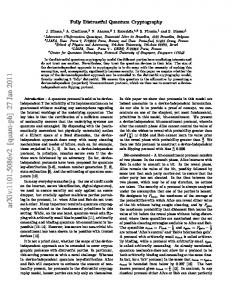
The procedure of BB84 is as follows (also shown in Table 1.1). 1. Quantum communication phase


LD 1 LD 2 LD 3 LD 4

5

SPD1 4x1 Optical Switch

CHANNEL

C W P

2x1 Optical Switch

ALICE

PBS1

HW P

BOB

SPD0 PBS2

SPD0

SPD1

Figure 1.1: Conceptual schematic for polarization-coding BB84 QKD system. LD: Laser Diode; CWP: Compensating Wave Plate; HWP: Half Wave Plate; PBS: Polarizing Beam Splitter; SPD: Single Photon Detector. Reproduced from [1]. ©2009 Springer. (a) In BB84, Alice sends Bob a sequence of photons, each independently chosen from one of the four polarizations—vertical, horizontal, 45-degrees and 135degrees. (b) For each photon, Bob randomly chooses one of the two measurement bases (rectilinear and diagonal) to perform a measurement. (c) Bob records his measurement bases and results. Bob publicly acknowledges his receipt of signals. 2. Public discussion phase (a) Alice broadcasts her bases of measurements. Bob broadcasts his bases of

Table 1.1: Procedure of BB84 protocol. Reproduced from [1]. ©2009 Springer. Alice’s bit sequence

1

Alice’s basis

Alice’s photon polarization

0

1

0

1

0

0

Bob’s basis Bob’s measured polarization

1

0

1

Bob’s sifted measured polarization

Bob’s data sequence

0

1

0

0

1


6

measurements. (b) Alice and Bob discard all events where they use different bases for a signal. The remaining bits are defined as “sifted bits”. (c) To test for tampering, Alice randomly chooses a fraction, p, of all remaining events as test events. For those test events, she publicly broadcasts their positions and polarizations. (d) Bob broadcasts the polarizations of the test events. (e) Alice and Bob compute the error rate of the test events (i.e., the fraction of data for which their values disagree). If the computed error rate is larger than some prescribed threshold value, say 11%, they abort. Otherwise, they proceed to the next step. (f) Alice and Bob each convert the polarization data of all remaining data into a binary string called a raw key (by, for example, mapping a vertical or 45degrees photon to “0” and a horizontal or 135-degrees photon to “1”). They can perform classical post-processing such as error correction and privacy amplification to generate a final key. A conceptual schematic of polarization coding BB84 implementation is shown in Figure 1.1. Four different polarization states at Alice’s side are generated by four laser diodes. A 4 1 optical switch is used to randomly pick one of the four states for each bit. Note that it is important for the classical communication channel between Alice and Bob to be authenticated. Otherwise, Eve can easily launch a man-in-the-middle attack by disguising herself as Alice to Bob and as Bob to Alice. Fortunately, authentication of an m-bit classical message requires only a logarithmic in m bit authentication key [26]. Therefore, QKD provides an efficient way to expand a short initial authentication key into a long key. By repeating QKD many times, one can get an arbitrarily long secure key.


7

PMB

PMA Laser Diode

BS1

BS2

CHANNEL

ALICE

BS3

BOB

BS4

SPD0

SPD1

Figure 1.2: Conceptual schematic for double Mach-Zehnder interferometer phase-coding BB84 QKD system. PM: Phase Modulator; BS: Beam Splitter; SPD: Single Photon Detector. Reproduced from [1]. ©2009 Springer.

1.2.2

Extending Polarization Coding to Phase Coding

Note that the BB84 protocol can be implemented with any two-level quantum system (qubits). In the above section, we have described the BB84 protocol in terms of polarization encoding. This is just one of the many possible types of encodings. Indeed, it should be noted that other encoding methods, particularly phase encoding, also exist. In phase encoding, a signal consists of a superposition of two time-separated pulses, known as the reference pulse and the signal pulse. The information is encoded in the relative phase º between the two pulses: i.e., the four possible states used by Alice are 1~ 2(SRe + SSe), º º º 1~ 2(SRe − SSe), 1~ 2(SRe + iSSe), 1~ 2(SRe − iSSe). A conceptual schematic for phase-coding BB84 implementation is shown in Figure 1.2. Note that, the phase encoding scheme is equivalent to the polarization encoding scheme mathematically. They are simply different embodiments of the same BB84 protocol.

1.2.3

Security Proof: Entanglement Distillation

There are several approaches to prove the security of BB84 [11] protocol. Here we will focus on the entanglement distillation approach, which is widely used. Entanglement distillation protocol (EDP) provides a simple approach to security proof


8

[27, 28, 29]. The basic insight is that entanglement is a sufficient (but not necessary) condition for a secure key. Consider the noiseless case for example. Suppose two distant parties, Alice and Bob, share a maximally entangled state of the form SφeAB =

º1 (S00e AB + 2

S11eAB ). If each of Alice and Bob measure their systems, then they will both get “0”s or “1”s, which is a shared random key. Moreover, if we consider the combined system of the three parties — Alice, Bob, and Eve — we can use a pure-state description in a larger Hilbert space and consider a pure state SψeABE . In this case, the von Neumann entropy [30] of Eve S(ρE ) = S(ρAB ) = 0. Here ρE and ρAB are density matrices for Eve and the joint system of Alice and Bob, respectively. This means that Eve has absolutely no information on the final key. This is the consequence of the standard Holevo’s theorem [31]. In the noisy case, Alice and Bob may share N pairs of qubits, which are a noisy version of N maximally entangled states. Now, using the idea of entanglement distillation protocol (EDP) [32], Alice and Bob may apply local operations and classical communications (LOCCs) to distill from the N noisy pairs a smaller number, say M , almost perfect aM

pairs, i.e. a state close to SφeAB . Once such an EDP has been performed, Alice and Bob can measure their respective systems to generate an M -bit final key. The above description of EDP is for a quantum-computing protocol where we assume that Alice and Bob can perform local quantum computations. In practice, Alice and Bob do not have large-scale quantum computers at their disposal. Shor and Preskill made the important observation that the security proof of the standard BB84 protocol can be reduced to that of an EDP-based QKD protocol [27, 28]. The Shor-Preskill proof [29] makes use of the Calderbank-Shor-Steane (CSS) code, which has the advantage of decoupling the quantum error correction procedure into two parts: bit-flip and phase error correction. They go on to show that bit-flip error correction corresponds to standard error correction and phase error correction corresponds to privacy amplification. Besides the entanglement distillation protocols, there are several other approaches to


9

prove the security of QKD. The communication complexity/quantum memory approach to security proof was proposed by Ben-Or [33] and subsequently by Renner and König [34]. See also [35]. The “twisted state” approach was presented in [36]. A clear and rigorous discussion of a complementary principle approach to security proof has recently been achieved by Koashi [37].

1.2.4

First Experimental Implementations

The proposal of BB84 [11] protocol seemed to be simple. However, the authors of [11] were not very interested in implementing this protocol experimentally. Without experimental demonstrations, researchers in other fields (e.g., conventional cryptography) became skeptical of the subject. Five years after the publication of [11], Bennett, Bessette, Brassard, Salvail, and Smolin decided to perform a simple QKD experiment to demonstrate its feasibility [38]. This first demonstration was based on polarization coding. Heavily attenuated laser pulses instead of single photons were used as quantum signals, which were transmitted over 30 cm of open air at a repetition rate of 10 Hz. 30 cm is not that appealing for practical communications. This short distance is largely due to the difficulty of optical alignment in free space. Switching the channel from open air to optical fibre is a natural choice. In 1993, Townsend, Rarity, and Tapster demonstrated the feasibility of phase-coding fibre-based QKD over 10km telecom fibre [39] while Muller, Breguet, and Gisin demonstrated the feasibility of polarization-coding fibre-based QKD over 1.1 km telecom fibre [40]. (Also, Jacobs and Franson demonstrated both free-space [41] and fibre-based QKD [42].) These are both feasibility demonstrations in which neither of them applied random basis selection at Bob’s side. P. D. Townsend demonstrated QKD with Bob’s random basis selection in 1994 [43]. It involved phase-coding and was over 10 km fibre. The source repetition rate was 105 MHz (which is quite high even by today’s standard) but the phase modulation rate was 1.05 MHz. This mismatch brought a question mark on its security.


1.2.5

10

Experimental Limits

Experimental implementations of QKD use imperfect real-life devices. Such imperfections bring many limits to QKD implementations. Here we will discuss the distance and counting rate limits. In other words, we will see why QKD cannot go very far or very fast. Short transmission distance is the most noticeable limit of BB84 implementations over classical optical communication implementations. The longest transmission distance of BB84 implementation is 144 km [44]. Other protocols have been implemented over longer distances of 200 km [22] and 250 km [45]. However, these distances are much shorter than standard optical communication distances, which can connect different continents. This is because extremely weak quantum signals (at the single photon level) propagating through a quantum channel (either in fibre or in free space) may be lost before reaching the receiver due to channel attenuation. Classical optical relay stations cannot amplify quantum signals due to the quantum no-cloning theorem [13, 14]. Methods to extend the transmission distances of QKD include establishing ground-satellite quantum link [46] or building up quantum repeaters [47]. Both solutions are challenging for current technology. Low key generation rate is another disadvantage of BB84 protocol. As we just discussed, weak quantum signals have high probability to be lost in the channel if Alice and Bob are far apart. For example, if Alice and Bob are connected with a 100 km standard telecom fibre, which has a loss coefficient α = −0.21 dB/km at 1550 nm [19], then the transmittance between Alice and Bob will be less than 1%. If Alice sets her average output intensity at 0.1 photons per pulse [19], the photons will hit Bob’s lab at a frequency that is three orders of magnitude lower than the pulse repetition rate at Alice’s side. Even if the pulse repetition rate at Alice’s side is as high as 10 GHz [22], photons will hit Bob’s lab at a frequency that is no greater than 10 MHz. Bob’s finite detection efficiency, error correction cost and privacy amplification cost will further reduce the final secure


11

ALICE

BOB EPR Source

Figure 1.3: Conceptual schematic of an entanglement-based QKD system with the source in the middle of Alice and Bob. Reproduced from [1]. ©2009 Springer. key generation rate. So far, the fastest key generation rate achieved for BB84 protocol is 1.02 Mbps at a distance of 20 km [48].

1.3

Other QKD Protocols

Given the popularity of the BB84 protocol, why should people be interested in other protocols? There are several reasons. An important one is that while it is possible to implement standard BB84 protocol with attenuated laser pulses, its performance in terms of key generation rate and distance is somewhat limited. The origin and consequences of this limit will be discussed in Section 1.4.1.

1.3.1

Entanglement-based Protocols

In 1991, Ekert proposed the first entanglement based QKD protocol, commonly called E91 [12]. The basic idea is to test the security of QKD by using the violation of Bell’s inequality. A standard approach is to put the entanglement source right in the middle of Alice and Bob. See Figure 1.3. Once an entangled pair is generated, the two particles are directed


DET

ALICE

12

EPR Source

BOB

Figure 1.4: Conceptual schematic of an entanglement-based QKD system with the source at Alice’s side. DET: Alice’s detection system. Reproduced from [1]. ©2009 Springer. to different destinations. Alice and Bob measure the particles locally, and keep the result as the bit value. This approach has potential in the ground-satellite intercontinental entanglement distribution, in which the entanglement source is carried by the satellite and the entangled photons are sent to two distant ground stations. A simpler version is to include the entanglement source in Alice’s side locally. See Figure 1.4. Once Alice generates an entangled pair, she keeps one particle and sends the other to Bob. Both Alice and Bob measure the particle locally and keep the result as the bit value. This approach is significantly simpler than the above design because only Bob needs the telescope and compensating parts. A recent experiment of source-in-Alice entanglement-based quantum communication over 144 km open air is reported in [49].

1.3.2

Decoy State Protocols

BB84 implemented with weak coherent state has a key generation rate that scales only quadratically with the transmittance [50, 51]. The decoy state protocol can dramatically increase the key generation rate so that it scales linearly with the transmittance. Details of decoy state protocols are discussed in Chapter 2.

1.3.3

Gaussian-modulated Coherent State (GMCS) Protocol

Instead of using discrete qubit states as in the BB84 protocol, one may also use continuous variables for QKD. Gaussian-modulated coherent states have been proposed for QKD.


AM Laser Diode

13

PMA

BS1

PMB

BS2

CHANNEL

ALICE

BS3

BOB

HD

BS4 PD

PD

-

Figure 1.5: Conceptual schematic for Gaussian-modulated Coherent State QKD system. PM: Phase Modulator; AM: Amplitude Modulator; BS: Beam Splitter; PD: Photo Diode; HD: Homodyne Detector (inside dashed box). Reproduced from [1]. ©2009 Springer. In GMCS QKD, Alice sends Bob a sequence of coherent state signals. For each signal, Alice draws two random numbers XA and PA and sends a coherent state SXA + iPA e to Bob. Bob randomly chooses to measure either the X quadrature of the P quadrature with a phase modulator and a homodyne detector. An advantage of a GMCS QKD is that every signal can be used to generate a key, whereas in qubit-based QKD such as the BB84 protocol, losses can substantially reduce the key generation rate. Therefore, it is widely believed that for short-distance (say < 15 km) applications, GMCS QKD may give a higher key generation rate.

1.3.4

Differential-phase-shift-keying (DPSK) Protocols

In DPSK protocol, a sequence of weak coherent state pulses is sent from Alice to Bob. The key bit is encoded in the relative phase of the adjacent pulses. Therefore, each pulse belongs to two signals. DPSK protocol is simpler in hardware design than the BB84 [11] protocol as it requires only one Mach-Zehnder interferometer and one phase modulator. See Figure 1.6. While DPSK protocol is simpler to implement than BB84, a full proof of its unconditional security is still missing3 . Therefore, it is hard to quantify its secure key generation 3

Some security proofs of DPSK protocol under certain additional assumptions, like the single photon source assumption [52], or the zero-error assumption [53], have been developed.


Laser Diode

PM

14

CHANNEL

ALICE

BS1

BOB

BS2

SPD0

SPD1

Figure 1.6: Conceptual schematic for differential phase shift keying QKD system. PM: Phase Modulator; BS: Beam Splitter; SPD: Single Photon Detector. Reproduced from [1]. ©2009 Springer. rate and perform a fair comparison with, for example, decoy state BB84 protocol. Attacks against DPSK has been studied in, for example, [54, 55].

1.4

Assumptions in Quantum Cryptography

Quantum cryptography is proved to be unconditionally secure. Here we emphasize that “unconditionally secure” does not imply “absolutely secure”. “Unconditional” in the security proof of QKD means that no assumption about Eve’s technology is made, except that quantum mechanics is correct. However, we do have to make assumptions on Alice’s and Bob’s sides to ensure the security. The concept of unconditional security in QKD is discussed in detail in [56]. If the assumptions on Alice’s and/or Bob’s sides are violated, the security of QKD can be breached.

1.4.1

Single Photon Source Assumption

The original BB84 [11] proposal required a single photon source. However, most QKD implementations are based on faint lasers due to the great challenge to build perfect single photon sources. In 2000, the security of coherent laser based QKD systems was analyzed first against individual attacks [57]. Finally, the unconditional security of coherent laser based QKD systems was proven in 2001 [51] and in a more general setting in 2002 [50].


15

Gobby, Yuan, and Shields demonstrated an experiment based on [57] in 2005 [58]. Note that this work was claimed to be unconditionally secure. However, due to the limit of [57], this is only true against individual attacks rather than the most general attack. The security analysis in [51, 50] will severely limit the performance of unconditionally secure QKD systems. Fortunately, since 2003 the decoy state method [59, 60, 61, 62, 63, 64] has been proposed by Hwang and extensively analyzed by our group at the University of Toronto and by Wang. The first experimental demonstration of decoy state QKD was reported by us in 2006 [65] over 15 km telecom fibre and later over 60 km telecom fibre [66]. Subsequently, decoy state QKD was further demonstrated by several other groups [44, 67, 68, 69, 70]. Details of our decoy state QKD work is presented in Chapter 24 .

1.4.2

Phase Randomization Assumption

Phase randomization is an assumption that is widely made in many security proofs, including the security proof of decoy state protocols [50, 51, 61]. Phase randomization can transform a general photonic state into a classical mixture of Fock states: ρ = Pn pn Sne`nS. A significant advantage of making such an assumption is that one can argue that some optical signals sent from Alice contain exactly one photon (i.e., in single-photon state). For these single photon qubits, one can apply security proofs of single photon BB84 protocol [28, 29, 71]. It is shown that [72] non-phase randomized BB84 protocol yields a lower final key rate than phase-randomized BB84 protocol does. In other words, if phase randomization assumption is violated, and Alice and Bob do not know it, Eve can learn more information than Alice and Bob expect. As an important assumption in security proofs, phase randomization receives little attention in experimental implementations. It has never been actively enforced in experiments until our demonstration [73]. Details of our experimental demonstration of QKD 4

Chapter 2 is largely based on [65, 66], of which I am the first author.


16

with active phase randomization are discussed in Chapter 35 .

1.4.3

Coherent State Assumption

It is widely assumed in many security proofs (eg., Ref. [50, 51, 61]) that Alice sends out phase-randomized coherent states. In other words, photon numbers of all signals sent from Alice obey Poisson distribution. If this assumption is valid, Alice and Bob know the probability that Alice sends out a single-photon signal. This can substantially simplify the security analysis of laser-based QKD implementations. The validity of the coherent state assumption is questionable. For example, it is common to use pulsed laser diodes as sources in QKD experiments. These laser diodes are driven by pulsed electrical currents. When the driving current is switched on, it will take a short while before the laser’s gain reaches its stabilizing threshold. During this transition period, the output from the diode cannot be viewed as a coherent state. Therefore, it is not rigorous to consider the entire pulse as a coherent state. A more severe problem comes from the standard bi-directional (so-called “plug & play”) design [74], which is widely used in commercial QKD systems. In this particular scheme, bright pulses are generated by Bob rather than Alice. The pulses will travel through the channel, which is fully controlled by Eve (an eavesdropper), before entering Alice’s lab to get encoded and sent back to Bob. Eve can perform arbitrary operations on the pulses when they are sent from Bob to Alice. In the worst case, Eve can replace the original pulses by her own sophisticatedly prepared optical signals. Such an attack is called the Trojan horse attack [75]. Therefore, it is not safe to assume that Alice uses a coherent state source in the security analysis of “plug & play” QKD systems. We developed a security proof that does not require this coherent state assumption. Our security proof is applicable to the worst case where the source is controlled by Eve. 5

Chapter 3 is largely based on [73], of which I am the first author.


17

Details of our security proof are presented in Chapter 4 and 56 .

1.4.4

Identical Detector Efficiency Assumption

In most BB84 QKD implementations, two or more SPDs are used. It is widely assumed that all the SPDs have identical detection efficiencies. This assumption is often verified by checking if Bob’s sifted key bits have similar numbers of “0”s and “1”s. Several proposals of side-channel attacks [78, 79, 80] made it possible to violate this assumption without being caught. That is, Eve can subtly manipulate Bob’s detection system such that for each individual bit, SPDs have substantial detection efficiency mismatch. Moreover, Eve can make sure that Bob still sees similar counts of “0”s and “1”s statistically. We demonstrated time-shift attack experimentally [81] to illustrate the feasibility and consequence of violating the identical detector efficiency assumption. Our attack was done on a commercial QKD system [24], thus highlighting the vulnerabilities of even well-designed commercial QKD systems. Details of our experimental quantum hacking work are presented in Chapter 67 .

1.4.5

Other Assumptions

There are many other assumptions made in various security proofs. A crucial one may be the single-mode assumption. That is, it is assumed that Bob has a strong filter that is transparent to only one optical mode. This assumption has not been experimentally enforced yet. It is unclear how to build a practical filter that is completely opaque to all but one optical mode. On the other hand, it is challenging to prove the security of a QKD system if multi-mode contribution is allowed. 6

Chapter 4 is largely based on [76], and Chapter 5 is largely based on [77]. I am the first author of both papers. 7 Chapter 6 is largely based on [81], of which I am the first author.


18

It is widely assumed in many security proofs that side-channels do not exist. Violation of this assumption is reported in several experiments [81, 82]. Security proof considering some side-channels has been developed [83]. However, a security proof of practical QKD system against the most general side-channel attack is yet to be developed.

1.4.6

Can We Remove the Assumptions?

Recently, there has been much academic interest on the connection between the security of QKD and fundamental physical principles such as the violation of Bell’s inequality. An ultimate goal, which has not yet been achieved [84], is to construct a device-independent security proof. That is, one does not make any assumption about Alice’s and Bob’s local devices. The security is based purely on the violation of Bell-inequalities. Testing Bell-inequalities with high fidelity requires very high detection efficiency (A 82.8%, including channel loss). This is not practical for current single photon detectors and channels. If detection efficiency is not high enough, local hidden variable model can be constructed and the violation of Bell-inequalities does not imply non-locality. A fair sampling assumption may save the day. That is, one may assume that all the detection events are a fair sample from all the photon creation events. However, as we show in Chapter 6, the low detection efficiency of practical detectors not only violates the fair sampling assumption that would be needed in security proofs based on Bellinequality violation, but also gives Eve (an eavesdropper) a powerful handle to break the security of a practical QKD system. Therefore, the detection efficiency loophole is of both conceptual and practical interest. Recently, it is shown in [85] that for BB84, a detection efficiency of 50% is enough for security proofs against detection efficiency mismatch.


1.5

19

Outline

This thesis is organized in the following way: • In Chapter 2, the first decoy state QKD experiments are presented. These works are published in [65, 66], and I am the first author for both papers. These successful demonstrations show that it is possible to implement unconditionally secure QKD with a weak coherent source. The single photon source assumption can then be removed. I was the chief experimental contributor to this work. I also implemented the numerical simulation that is presented in Section 2.3 (I acknowledge that the algorithm for the simulation was developed by Dr. Xiongfeng Ma). Part of the experiment (which is published in [65]) was performed when I was an M. Sc. student at University of Toronto. Most of the write-up of [65] was completed during my Ph. D. study. • In Chapter 3, the first active phase randomization experiment in QKD is presented. This work is published in [73], and I am the first author. This demonstration shows that the phase randomization assumption, which is required by decoy state QKD, can be experimentally guaranteed. I designed a polarization insensitive phase modulator, and synchronized it with our commercial QKD system to implement phase randomization. I also proposed and implemented a way to verify the phase randomization. • In Chapter 4, the first security proof of QKD with an unknown and untrusted source is presented. This work is published in [76], and I am the first author. I developed a security proof which shows that the coherent state assumption, which is assumed in many security proofs including the ones for decoy state QKD, can be removed. I also developed some numerical simulation techniques. • In Chapter 5, the results shown in Chapter 4 are improved. This work is now


20

under journal review [77], and I am the first author. I developed an improved protocol which is a lot simpler to implement than the protocol proposed in Chapter 4. I implemented extensive numerical simulations. Several key imperfections for practical devices are considered. • In Chapter 6, the first successful quantum hacking experiment against a commercial QKD system is presented. This work is published in [81], and I am the first author. I performed the experiment and acquired the results. Here I acknowledge that Dr. Chi-Hang Fred Fung also made substantial contributions to this work, especially in analyzing the experimental results. The demonstration shows that the identical detector efficiency assumption can be violated due to Eve’s malicious operations. • In Chapter 7, we conclude the thesis with a summary and an outlook of QKD research.

1.6

Publications Related to This Thesis

1. Y. Zhao, B. Qi, X. Ma, H.-K. Lo, and L. Qian. Experimental quantum key distribution with decoy states. Phys. Rev. Lett., 96:070502, 2006. 2. Y. Zhao, B. Qi, X. Ma, H.-K. Lo, and L. Qian. Simulation and implementation of decoy state quantum key distribution over 60 km telecom fiber. In Proceedings of IEEE International Symposium of Information Theory, pages 2094–2098. IEEE, 2006. 3. Y. Zhao, B. Qi, and H.-K. Lo. Experimental quantum key distribution with active phase randomization. Appl. Phys. Lett., 90:044106, 2007. 4. Y. Zhao, B. Qi, and H.-K. Lo. Quantum key distribution with an unknown and untrusted source. Phys. Rev. A, 77:052327, 2008.


21

5. Y. Zhao, C.-H. F. Fung, B. Qi, C. Chen, and H.-K. Lo. Quantum hacking: experimental demonstration of time-shift attack against practical quantum key distribution system. Phys. Rev. A, 78:042333, 2008. 6. Y. Zhao, B. Qi, H.-K. Lo, and L. Qian. Passive estimate of an untrusted source for quantum key distribution. arXiv:0905.4225, submitted to New J. Phys., 2009. 7. H.-K. Lo and Y. Zhao. Quantum cryptography. in Encyclopedia of Complexity and System Science (Springer, New York, 2009), Vol. 8, pp. 7265–7289.

Chapter 2 Decoy State QKD: Simulation and Experiment It is assumed in many security proofs of QKD [28, 29, 71] that Alice possesses a perfect single photon source. However, most QKD implementations are based on faint laser sources due to the great challenge to build perfect single photon sources. Decoy state method is proposed as a novel solution to substantially improve the performance of weak coherent state based QKD without jeopardizing the security. In this chapter, we first introduce the basic concepts of decoy state QKD. We then present the experimental demonstrations of two decoy state protocols. Numerical simulations of decoy state QKD are performed. The techniques in the numerical simulations is also discussed. The content of this chapter is largely based on [65, 66], of which I am the first author.

2.1

Introduction

The security of QKD was proved based on the fundamental laws of quantum physics assuming a perfect single photon source is utilized [28, 29, 71]. Unfortunately, in view of implementation, the “perfect” devices are always very hard to build. Therefore, most 22

Chapter 2. Decoy State QKD: Simulation and Experiment

23

up-to-date QKD systems substitute the desired perfect single photon sources by heavily attenuated coherent laser sources. QKD can be performed with these laser sources over more than 250 km of telecom fibres [45]. However, this substitution raises some severe security concerns. The output photon number per pulse of a coherent laser source obeys Poisson distribution. Thus the occasional production of multi-photon signals is inevitable no matter how heavily one attenuates the laser. This occasional production of multi-photon signals opens a back door for Eve to launch some sophisticated attacks, like the photon-number-splitting (PNS) attack [86]. The PNS attack works in the following manner [86]: Eve can first perform a quantum non-demolition (QND) measurement on the photon number of each signal. Eve then selectively suppresses all the single photon signals from Alice, and splits all the multiphoton signals by keeping one copy herself and sending the other copy to Bob. In this way, Eve could have an identical copy of what Bob possesses. She keeps all the qubits in her quantum memory until Alice broadcasts the correct basis for each qubit. Eve can then measure her qubits accordingly, thus breaking the security of BB84 protocol. Although such an attack may appear to be beyond current technology, the first rule in cryptography is: never underestimate the determination and ingenuity of your opponents in breaking your codes. Is it possible to develop some special measure that can make QKD secure even with some practical systems? The answer is yes. From physical intuition, if Alice sends out a single photon signal, and Bob luckily receives it, this bit (normally defined as in “single photon state”) should be secure, because Eve cannot split or clone it. Based on this intuition, rigorous security analysis on some practical QKD system is proposed by [51] and Gottesman-Lo-L¨ utkenhaus-Preskill (GLLP)[50], which is based on the entanglement distillation approach to the security proofs. The main idea of GLLP’s work is not to find which signals are secure (i.e., single-


24

photon signals), because it would be beyond current technology. Instead, GLLP shows that the ratio of secure signals can be estimated from some experimental parameters, and the secure key bits can then be extracted from the raw key based on this ratio through the data post-processing. The secure key generation rate R, which is defined as the ratio of the length of the secure key to the total number of signals sent by Alice, is given by [50] R C q−Qµ f (Eµ )H2 (Eµ ) + Q1 [1 − H2 (e1 )],

(2.1)

where q depends on the protocol; the subscript µ is the average photon number per signal in the signal states; Qµ and Eµ are the gain and the quantum bit error rate (QBER) of the signal states, respectively; Q1 and e1 are the gain and the error rate of the single photon state in the signal states, respectively; f (x) is the bi-directional error correction inefficiency [87]; and H2 (x) is the binary entropy function: H2 (x) = −x log2 (x) − (1 − x) log2 (1 − x). Qµ and Eµ can both be measured directly from the experiments, while Q1 and e1 have to be estimated (because Alice and Bob could not measure the photon number of each pulse with current technology). Here we define “gain” as the ratio of the number of Bob’s detection events to the number of signals emitted by Alice in the cases where Alice and Bob use the same basis. It depends mainly on the intensity of signal, the channel transmittance, and Bob’s quantum efficiency. GLLP [50] has also given a method to estimate the lower bound of Q1 and the upper bound of e1 , thus giving out the lower bound of the key rate R. However, with the coherent laser sources, these bounds are not tight. It follows that the security of practical QKD set-ups can be guaranteed only at very short distances and very low key generation rates [50, 61]. A key question is thus raised: How can one extend both the maximum secure distance and the key generation rate of QKD? The most intuitive choice would be to use a (nearly) perfect single photon source. Despite much experimental effort, reliable near-perfect single photon sources are far from practical [88, 89].


25

Another solution to increase the maximum secure distance and the highest key generation rate is to employ decoy states, using some extra states of different average photon numbers to detect photon-number dependent attenuation. The decoy method was first discovered by Hwang who proposed using strong pulses as decoys [59]. The idea of using weak pulses as decoys is proposed by Lo [60]. The first rigorous security proof of decoy state QKD was presented by Lo, Ma and Chen [61]. It is shown that the decoy state method can be combined with standard GLLP result to achieve dramatically higher key generation rates and longer distances [61]. Moreover, practical protocols with vacua and weak coherent states as decoys were proposed [60]. Subsequently, we have analyzed the security of practical protocols [62]. Decoy method was also studied by Wang [63, 64]. The basic idea of decoy state QKD is as follows: Alice introduces some “decoy” states with average photon numbers νi besides the signal state with average photon number µ (x νi ). Each pulse sent by Alice is assigned to a state (signal state or one of the decoy states) randomly. Alice then modulates the amplitude of each pulse according to its state. All the pulses are then sent to Bob through the quantum channel. Alice announces the state of each pulse after Bob’s acknowledgment of receipt of the signals. The statistical characteristics (i.e., the gain and the QBER) of each state can then be analyzed separately. Note that the average photon number of certain state is only by statistical meaning, while Eve’s knowledge is limited to the actual photon number in each individual pulse. Therefore, Eve has no clue about the state (signal or decoy) of each pulse. Eve’s attack will modify the statistical characteristics (gain or QBER) of the decoy states and/or the signal state and will be caught. The decoy states are used only for catching an eavesdropper, but not for the key generation. It has been shown [61, 62, 63, 64] that, in theory, decoy state QKD can substantially enhance the security and the performance of QKD. The power and the feasibility of the decoy method can be shown only by implementing it. To implement the decoy state QKD, it is intuitive to utilize variable optical attenuators


APD

LD APD

Φ

50ns

15km CG DG PD FM

B

CA DA

DL

PBS

BOB

26

ALICE

Φ

A

Jr. Alice

Figure 2.1: Schematic of the set-up in one-decoy protocol experiment. Inside Bob/Jr. Alice: components in Bob/Alice’s package of id Quantique QKD system. Our modifications: CA: Compensating AOM; CG: Compensating Generator; DA: Decoy AOM; DG: Decoy Generator. Original QKD system: LD: Laser Diode; APD: Avalanche Photon Diode; Φi : Phase Modulator; PBS: Polarization Beam Splitter; PD: Classical Photo Detector; DL: Delay Line; FM: Faraday Mirror. Solid line: SMF28 single mode optical fibre; dashed line: electric cable. Reproduced from [65]. ©2006 American Physical Society. (VOAs) to modulate the intensity of each signal to that of its state. Actually, this is exactly the way we used.

2.2

Implementations of Decoy State Protocols

In [60, 61, 62], we have proposed several protocols on decoy state QKD. The most important two protocols are the one-decoy protocol (the simplest protocol) and the weak+vacuum protocol (the optimal protocol). We have implemented both of them, over 15 km (the one-decoy protocol) and 60 km (the weak+vacuum protocol) standard telecom fibres. Decoy state protocols were also studied by Wang [63, 64].

2.2.1

Implementation of one-decoy protocol

In one-decoy protocol, only one decoy state with average photon number per signal ν < µ is needed. Alice could decide the values of µ and ν, and the ratio of number of pulses


27

used as decoy state to that of total pulses, then randomly assign the state to each signal by attenuating the intensity of each signal to either µ or ν. We implemented the one-decoy protocol by adding acousto-optical modulators (AOMs, including CA, DA in Figure 2.1) to a commercial “Plug & Play” QKD system manufactured by id Quantique (Jr. Alice and Bob in Figure 2.1). We choose AOM to modulate the signals because we need this amplitude modulation to be polarization insensitive. This QKD system is based on a 1550 nm laser source with pulse repetition rate of 5 MHz. Its intrinsic parameters, including dark count rate Y0 , detector error rate edetector , and Bob’s quantum efficiency ηBob are listed on Table 2.1. Before the experiment, we perform a numerical simulation (discussed in detail in Section 2.3) with the parameters of our set-up as in Table 2.1 and optimally set µ and ν to 0.80 and 0.120 photons, respectively. The actual distribution of the states is produced by an id Quantique Quantum Random Number Generator. Around 10% of the signals are assigned as the decoy states as suggested by the numerical simulation. This random pattern is generated and loaded to the Decoy Generator (DG in Figure 2.1) before the experiment. Here we describe the flow of the experiment: 1. Bob generates a chain of strong laser pulses by the laser diode (LD in Figure 2.1) Table 2.1: Some intrinsic parameters of the QKD system. These parameters are different for the two implementations because the single photon detectors of the QKD system were adjusted by the manufacturer between the two experiments. Reproduced from [66] with permission. ©2006 IEEE.

Implementation

Y0

edetector

ηBob

One-Decoy

2.11 10−5

8.27 10−3

2.27 10−2

Weak+Vacuum

6.14 10−5

1.38 10−2

5.82 10−2


28

and sends them to Alice through the 15 km fibre. 2. The pulses propagate through the AOMs (CA and DA in Figure 2.1, the function of CA as well as CG is discussed in the next paragraph), whose transmittances are set to maximum at this period. 3. Each pulse is splitted by a coupler. Part of the input pulse will be detected by a classical photo detector (PD in Figure 2.1), which generates synchronizing signal to trigger the Decoy Generator (DG in Figure 2.1). 4. The generator holds for certain time period, during which the pulses are reflected by the faraday mirror (FM in Figure 2.1) and quantum information is encoded by the phase modulator (ΦA in Figure 2.1). 5. Here comes the key point: Decoy Generator (DG in Figure 2.1) will drive the Decoy AOM (DA in Figure 2.1) to modulate each pulse to the intensity (either 0.80 or 0.120) of the state it is assigned to exactly when the pulse propagates through the AOM. 6. The pulses (now in single photon level) return to Bob through the 15 km fibre again. 7. Bob decodes the quantum information by modulating the phases of the pulses by the phase modulator (ΦB in Figure 2.1) and see which single photon detector (APD in Figure 2.1) fires. The use of the Decoy AOM (DA in Figure 2.1) shifts the frequency of the laser pulses. Note that each qubit consists of two pulses that propagate through different arms of an asymmetric Mach-Zehnder interferometer. This frequency shift introduced by the AOM is then translated into a shift of relative phase between these two pulses. This phase shift increases QBER.


29

To compensate this phase shift, another AOM, the “Compensating AOM” (CA in Figure 2.1) is employed. The frequency of this compensating AOM is finely tuned such that the total phase shift becomes multiples of 2π. This compensation eliminates any additional QBER introduced by the frequency shift. This compensating AOM is driven by a second function generator, “Compensating Generator” (CG in Figure 2.1). Its transmittance is set constant throughout the experiment. Here we emphasize that the holding time of the Decoy Generator (DG in Figure 2.1) after being triggered by the photo detector (PD in Figure 2.1) must be very precise, because same modulation must be applied to the two pulses of the same signal to keep visibility high. In our experiment, the precision of this holding time is 10 ns. After Bob’s receipt of all the signals, Alice broadcasted to Bob the distribution of decoy states as well as basis information. Bob then announced which signals he had actually received in correct basis. We assume Alice and Bob announced the measurement outcomes of all decoy states as well as a subset of the signal states. From those experimental data, Alice and Bob then determined Qµ , Qν Eµ , and Eν , whose values are now listed in Table 2.2. Note that our experiment is based on BB84 [11] protocol, thus q = NµS ~N , where NµS is the number of pulses used as signal state when Alice and Bob chose the same basis, and N = 105 Mbit is the total number of pulses sent by Alice in this experiment. Now we have to analyze the experimental result and estimate the lower bound of key generation rate R. This can be done by simply inputting the results in Table 2.2 to the following equations [62]: 2 2 2 µ2 e−µ L ν µν µµ − ν (Q e − Q e − E Q e ) µ µ µ µν − ν 2 ν µ2 e 0 µ2 Eµ Qµ , e1 B eU1 = QL1

Q1 C QL1 =

(2.2)

in which uα ), QLν = Qν (1 − º Nν Qν

(2.3)


30

where Nν is the number of pulses used as decoy states, and e0 (=1/2) is the error rate for the vacuum signal and therefore the lower bound of key generation rate is R C RL = q−Qµ f (Eµ )H2 (Eµ ) + QL1 [1 − H2 (eU1 )]

(2.4)

In our analysis of experimental data, we estimated e1 and Q1 very conservatively as within 10 standard deviations (i.e., uα =10), which promises a confidence interval for statistical fluctuations of 1 − 1.5 10−23 . Even with our very conservative estimation of e1 and Q1 , we got a lower bound for the key generation rate RL = 3.6 10−4 per pulse, which means a final key length of about L = N R 38kbit. We also calculated Rperfect = 1.418 10−3 , the theoretical limit from the case of infinite data size and infinite decoy states protocol, by using Eq. (1). We remark that our lower bound RL is indeed good because it is greater than 1~4 of Rperfect .

2.2.2

Implementation of weak+vacuum protocol

Weak+Vacuum protocol is similar to one-decoy protocol except that it has one more decoy state: the vacuum state, which has zero intensity. The vacuum state is to detect the background count rate. We hereby use the same notation for intensities as in Subsection 2.2.1: µ for signal state and ν < µ for weak decoy state. Weak+Vacuum protocol is theoretically predicted to have higher performance than Table 2.2: Experimental results in one-decoy protocol. As required by GLLP [50], bit values for double detections are assigned randomly by the quantum random number generator. Reproduced from [65]. ©2006 American Physical Society.

Para.

Value

Para.

Value

Para.

Value

Qµ

8.757 10−3

Eµ

9.536 10−3

q

0.4478

Qν

1.360 10−3

Eν

2.689 10−2

f (Eµ ) [87]

B1.22


APD

Φ

LD APD

50ns

60km

FG PD FM

B

AOM

DL

PBS

BOB

31

ALICE

Φ

A

Jr. Alice

Figure 2.2: Schematic of the set-up in weak+vacuum protocol experiment. Inside Bob/Jr. Alice: components in Bob/Alice’s package of id Quantique QKD system. Our modifications: AOM: Decoy AOM; FG: Functional Generator. Original QKD system: LD: Laser Diode; APD: Avalanche Photon Diode; Φi : Phase Modulator; PBS: Polarization Beam Splitter; PD: Classical Photo Detector; DL: Delay Line; FM: Faraday Mirror. Solid line: SMF28 single mode optical fibre; dashed line: electric cable. Reproduced from [66] with permission. ©2006 IEEE. one-decoy protocol and is the optimal protocol in asymptotic case [61, 62]. Our numerical simulation (detailed discussion in Section 2.3) shows that for our set-up (as in Table 2.1), with data size of 105 Mbit, the maximum secure distance for one-decoy protocol is 59 km, while that of weak+vacuum protocol is 68 km, as shown in Figure 2.4. We chose 60 km telecom fibre to perform weak+vacuum protocol. The implementation of weak+vacuum protocol requires amplitude modulation of three levels: µ, ν and 0. Note that it would be quite hard for high-speed amplitude Table 2.3: The experimental results of weak+vacuum protocol. Reproduced from [66] with permission. ©2006 IEEE. Para.

Value

Para.

Value

Qµ

1.81 10−3

Eµ

3.05 10−2

Qν

5.47 10−4

Eν

7.78 10−2

Y0

6.02 10−5

e0

0.51

q

0.319

f (Eµ )[87]

B 1.22


32

modulators to prepare the real “vacuum” state due to finite distinction ratio. However, if the gain of the “vacuum” state is very close (like within a few standard deviations) to the dark count rate, it would be a good approximation. Our set-up to implement weak+vacuum protocol (Figure 2.2) is very similar to that of one-decoy protocol (Figure 2.1) except for the absence of the “compensating” parts (CA & CG in Figure 2.1). This is because the frequency of the AOM (AOM in Figure 2.2) has been precisely adjusted to the value that the phase shift caused by it is exactly multiples of 2π. In other words, this AOM is self-compensated for our set-up. We performed numerical simulation (as discussed in details in Section 2.3) to find out the optimal parameters. According to simulation results, we choose the intensities as µ = 0.55, ν = 0.152. Numbers of pulses used as signal state, weak decoy state and vacuum state are Nµ = 0.635N , Nν = 0.203N , and N0 = 0.162N , respectively, where N = 105 Mbit is the total data size we used. The experimental results are shown in Table 2.3. Note that the gain of vacuum state (Y0 in Table 2.3) is indeed very close to the dark count rate (Y0 in Table 2.1, third row), therefore the vacuum state in our experiment is quite “vacuum”. We could estimate the lower bound of Q1 and upper bound of e1 by plugging these experimental results into the following equations [62]: 2 2 2 µ2 e−µ L ν µν Uµ −ν (Q e − Q e − Y ), µ 0 µν − ν 2 ν µ2 µ2 Eµ Qµ − e0 Y0L e−µ e1 B eU1 = , QL1

Q1 C QL1 =

in which

uα ), N0 Y 0 uα = Y0 (1 + º ), N0 Y 0

(2.5)

Y0L = Y0 (1 − º Y0U

(2.6)

and QLν takes the value as in Eq. (2.3). Again, we estimate Q1 and e1 very conservatively by setting uα = 10, which promises a confidence interval for statistical fluctuations of 1 − 1.5 10−23 .


33

A lower bound of the key generation rate RL = 8.45 10−5 per pulse is found by plugging the results of Eqs. (2.5) into Eq. (2.4), which means a final key length of about L = N R 9 kbit. Note that, one-decoy protocol cannot give out a positive key rate at 60 km as suggested by numerical simulation. Therefore, weak+vacuum protocol is in demand at this distance.We also confirm the numerical simulation result by plugging Qµ , Eµ , Qν and q from Table 2.3 into Eqs. (2.2)(2.3)(2.4) and found indeed that no positive key rate could be found.

2.3

Numerical Simulation

Numerical simulation is crucial for setting optimal experimental parameters and choosing the distance to perform certain decoy method protocol. Here we explain the principle of our simulation, and show some results. The principle of numerical simulation is that for certain QKD set-up, if the intensities and percentages of signal state and decoy states are chosen, we could simulate the experimental results (gains and QBERs of all states). For example, suppose we have a QKD set-up with transmittance η, detector error rate edetector and dark count rate Y0 , if the output intensity is set to be µ photons per signal, the gain and QBER of this state is expected to be [57] Qµ = Y0 + 1 − e−ηµ , 1 Eµ = (e0 Y0 + edetector (1 − e−ηµ )), Qµ

(2.7)

respectively. With these simulated experimental outcome, we could estimate the lower bound of the key generation rate. In experiment, it is natural to choose the intensities and percentages of signal state and decoy states which could give out the maximum key generation rate. This search for optimal parameters can be done by numerical simulation and exhaustive search. For example, we could try the values of µ and νi , the intensities of signal state and decoy


34

−2

Key Generation Rate (per pulse)

10

−3

10

−4

10

−5

10

−6

10

−7

10

Theoretical Limit Weak + Vacuum One Decoy GLLP (no decoy)

−8

10

−9

10

0

10

20

30

40

50

60

70

80

90

100

Distance (km)

Figure 2.3: Simulation result of the set-up on which we implemented the one-decoy protocol. Intrinsic parameters for this set-up is shown in the second row of Table 2.1. Solid line: the theoretical limit of key generation rate. Its maximum transmission distance is about 90 km. Dashed line: the performance of weak+vacuum protocol. Its maximum distance is about 70 km. Dotted line: the performance of one-decoy protocol. Its maximum distance is about 64 km. Dashed and dotted line: the performance without decoy method. Its maximum distance is only 9.5 km. Reproduced from [66] with permission. ©2006 IEEE. states, in the range of [0, 1] with a step increase of 0.001. Similar strategy can be applied on the percentage of each state. With certain combination of intensities and percentages, the gains and QBERs of different states could be simulated by Eqs. (2.7), and the key generation rate can be estimated by the chosen protocol, like Eqs. (2.2)(2.3)(2.4) for one-decoy protocol and Eqs. (2.3)(2.4)(2.5)(2.6) for weak+vacuum protocol. We can therefore find out the optimal combination that can give maximum key generation rate. Numerical simulation can also give the maximum secure distance for certain decoy protocol and QKD set-up. The transmittance of the system is a simple function of


35

distance [57] η = ηBob e−αl , where α(=0.21 dB/km in our set-up) is the loss coefficient. For a QKD set-up with known ηBob , α, edetector , and Y0 , we could find out the maximum key generation rate of some protocol at distance l. The shortest distance at which the maximum key generation rate for certain protocol hits zero is defined as maximum secure distance for this protocol on this set-up. It would probably be a waste of time to perform certain decoy state protocol far beyond its maximum secure distance. We performed numerical simulation based on the set-up on which we implemented the one-decoy protocol. The result is shown in Figure 2.3. The power of decoy method is explicitly shown by the fact that the maximum distance in the absence of decoy method is only 9.5 km. In other words, at 15 km, not even a single bit could be shared between Alice and Bob with guaranteed security. In contrast, with decoy states, our QKD set-up can be made secure over 60 km, which is substantially larger than the secure distance (9.5 km) without decoy states. The set-up on which we implemented the weak+vacuum protocol is a bit different from the one we implemented the one-decoy protocol because the single photon detector had been adjusted by the manufacturer and several important properties, including ηBob , Y0 and edetector , were changed, as shown in Table 2.1. The simulation result for this “new” set-up is shown in Figure 2.4. Clearly, the expected performance, including the key rate of certain distance and maximum secure distance of certain protocol, of this set-up is different from the previous one. This difference is natural because the properties of the system have changed. The advantage of weak+vacuum protocol over one-decoy protocol is shown by the fact that the maximum secure distance of one-decoy protocol is 59 km, which means that one-decoy protocol cannot give out a positive key rate at 60 km. We confirmed this numerical simulation result by plugging experimental results Qµ , Eµ , Qν and q from Table 2.3 into Eqs. (2.2)(2.3)(2.4) and found indeed that key rate is not positive. The maximum secure distance of our set-up is limited by equipment, especially the


36

−2


10

−3

10

−4

10

−5

10

−6

10

−7

10

−8

Theoretical Limit Weak + Vacuum One Decoy GLLP (no decoy)

10

−9

10

−10

10

0

10

20

30

40

50

60

70

80

90

Distance (km)

Figure 2.4: Simulation result of the set-up on which we implemented the weak+vacuum protocol. The intrinsic parameters of this set-up is shown in the third row of Table 2.1. Note that this set-up is different from the one we implemented one-decoy as reflected by the fact that in Table 2.1, the values in row 3 are different from the values in row 2. Solid line: the theoretical limit of key generation rate. Its maximum transmission distance is about 84 km. Dashed line: the performance of weak+vacuum protocol. Its maximum distance is about 68 km. Dotted line: the performance of one-decoy protocol. Its maximum distance is about 59 km. Dashed and dotted line: the performance without decoy method. Its maximum distance is only 14 km. Reproduced from [66] with permission. ©2006 IEEE.

single photon detectors we used (APDs in Figures 2.1&2.2). Given a better set-up (higher ηBob , lower edetector and Y0 ), secure decoy state QKD can be experimentally implemented over 100 km, as shown in [62].


2.4

37

Conclusion

For the first time, we have implemented decoy state QKD. We have implemented two protocols: The one-decoy protocol and the weak+vacuum protocol [62]. Simple modifications (adding AOMs) on a commercial QKD system are made to implement decoy state QKD. The simplicity of the modification (much simpler than building a near-perfect single photon source) shows the feasibility of decoy method. Also, the high key rates and long transmission distances (60 km) show the power of decoy method. Decoy method allows us to achieve much better performance with substantially higher key generation rate and longer distance than is otherwise possible. Given better QKD set-ups, decoy state method could make secure QKD at even longer distances. We conclude that, with careful conceptual design and optimization, decoy state QKD is easy to implement in experiments. It is, therefore, ready for immediate commercial applications.

2.5

Follow-up works on Decoy State QKD

Our work on experimental decoy state QKD triggered a wave of decoy state QKD implementations on various structures: D. Rosenberg et al. demonstrated decoy state QKD with superconductor single photon detectors over 102 km fibre [67]; C.-Z. Peng et al. demonstrated decoy state QKD with polarization coding over 107 km fibre [69]; Tobias Schmitt-Manderbach et al. demonstrated free-space decoy state QKD over a distance of 144 km [44]; Z.-L. Yuan et al. demonstrated a fibre-based decoy state QKD over 25 km [68]; and Z.-Q. Yin et al. demonstrated a fibre-based decoy state QKD over 130 km [70]. After a first wave of decoy state QKD demonstrations, several new advances were made in decoy state QKD. Continuous operating with automatic alignment techniques have been developed [90, 91], which are applied in field deployed fibre networks [92, 93]. Gigahertz decoy state QKD implementation is reported [48]. Decoy state protocols with a parametric down conversion (PDC) source have been proposed and experimentally


38

demonstrated [94, 95, 96]. As of today, decoy state method has become a standard technique to achieve high performance and high security QKD with weak coherent source. Decoy state QKD systems are commercially available now [23].

Chapter 3 Phase Randomization in QKD: Experiment Phase randomization is an important assumption made in many security proofs of practical quantum key distribution (QKD) systems. In particular, phase randomization is assumed in the security proof of decoy state QKD [61]. In this chapter, we present the first experimental demonstration of QKD with reliable active phase randomization. One key contribution is a polarization-insensitive phase modulator, which we add to a commercial phase-coding QKD system to randomize the global phase of each bit. We also propose and implement a useful method to verify the phase randomization experimentally. Our result shows very low quantum bit error rate (< 1%). The content of this chapter is largely based on [73], of which I am the first author.

3.1

Introduction

As we discussed in the last chapter, the single photon source assumption can be removed [50, 51] and the performance can still be very high since decoy state method has been proposed [59, 60, 61, 62, 63, 64] and implemented [65, 66]. However, this removal comes at a price of introducing another assumption: the phase of each quantum signal is uniformly 39

Chapter 3. Phase Randomization in QKD: Experiment

40

random [50, 51, 59, 60, 61, 62, 63, 64], and is inaccessible to the eavesdropper. Without phase randomization, one would have to use other techniques to prove the security of QKD [72], which yields a lower key rate. Moreover, it is unclear how to apply decoy state techniques without phase randomization. Phase randomization is an important assumption because any input state, after phase randomization, is transformed into a classical mixture of Fock states. Here we show it mathematically as follows: A general input optical state (in single mode) can be written as ρ0 = Q pm,n Sme`nS.

(3.1)

m,n

After phase randomization, this state is transformed as ρABE = Q pm,n Sme`nSei(m−n)θ ,

(3.2)

m,n

where θ is a random phase. Since this information is not available to Eve or Bob, the state sent from Alice will be ρBE = TrA ρABE =

2π 1 dθei(m−n)θ Q pm,n Sme`nS S 2π m,n 0

(3.3)

= Q pn,n Sne`nS. n

Until now, QKD experiments with intentionally randomized phase have never been reported. Here we remark that the quantum signals sent by Alice are not “naturally” phase-randomized. For example, in a uni-directional QKD system, strong ancillary pulses (sometimes called reference pulses) are sometimes used for feed-back control to stabilize the asymmetric Mach-Zehnder interferometer (MZI) [97]. The phase of such strong classical pulses could be (in principle) accurately measured, leaking the phase information to the eavesdropper. Even if weak signals are used, the phase coherence of the laser source could be maintained for many emissions of weak signals, which makes it possible to measure the phase accurately. For a bi-directional system (“plug & play” system) [98],


41

classical pulses sent from Bob cause the same problem as the strong ancillary pulses in a uni-directional system do. Active phase randomization in real QKD system is not entirely straightforward: the phase modulator should be polarization insensitive while usually it works only on one component of polarization; this extra phase modulator has to be carefully synchronized with the original system to randomize the phase of each individual bit; since the output from Alice is very weak ( 0.1 photons per pulse), it is not straightforward to verify that the phase is indeed randomized; the phase randomization must not increase the quantum bit error rate (QBER) significantly. In this chapter, we present the first QKD experiment with reliable active phase randomization. Our implementation is based on a modified commercial “plug & play” system [98]. The global phase of each bit is randomized by an additional phase modulator, after which the bit is sent to Bob. This phase modulator is designed to be polarizationinsensitive. Therefore, neither polarization-maintaining fibre nor dynamic polarization control is necessary. Our result shows that the phase difference between adjacent signals has been confidently randomized by this phase-randomization phase modulator, while the relative phase between the two pulses of the same signal is solely determined by Alice’s coding phase modulator. We expect phase randomization to become a standard part in future QKD systems due to its security significance [51, 50] and feasibility shown in this chapter.

3.2

Experiment

The schematic of our set-up is shown in Figure 3.1. The original QKD system works as follows: Bob generates a train of laser pulses at 5 MHz repetition rate; each pulse is split into two by an asymmetric MZI; the one that propagates through the shorter arm is called the reference pulse, and the one that propagates through the longer arm


APD

LD APD

Φ

FG

50ns

Φ

B

PI

PBS

BOB

ISL FC

42

ALICE

Φ

PD FM DL

Φ

A

Jr. Alice

FM

Figure 3.1: Upper Chart: Schematic of the experimental set-up in our system. Inside Bob/Jr. Alice: components in Bob/Alice’s package of id Quantique QKD system, respectively. Our modifications: ΦPI : polarization-insensitive phase modulator (detailed structure shown in lower chart); FG: function generator. Original QKD system: LD: laser diode; APD: avalanche photodiode; ΦA~B : phase modulator; PBS: polarization beam splitter; PD: classical photo detector; FM: faraday mirror. Lower chart: Detailed structure of the polarization-insensitive phase modulator. ISL: optical isolator; FC: 22 Fibre Coupler; Φ: electro-optical modulator; FM: faraday mirror. Solid line: optical fibre; dashed line: electric cable. Reproduced from [73] with permission. ©2007 American Institute of Physics.

is called the signal pulse; the insertion loss of the phase modulator (ΦB in Figure 3.1) makes the signal pulse weaker than the reference pulse. The state of the ith bit emitted from Bob is Sαi eSβi e, where Sαi e denotes the reference pulse and Sβi e denotes the signal pulse. Pulses are sent to Alice through the quantum channel; part of the pulses are split off to a photo detector (PD in Figure 3.1) for synchronization purposes, and the rest enter Alice and are reflected by a Faraday mirror (FM in Figure 3.1, upper chart); Alice


Φ

Φ

Φ

Bit 1

Bit 2

Bit 3

1

Φ

1

2

Φ

2

3

Φ

3

Ref. Pulse Sig. Pulse

H V

Φ

Bit 2

H

V

4

0

Bit 1

43

Bit 3

20

50 70

Modulation Moment (ns)

Figure 3.2: Upper chart: correctly implemented phase randomization. A different random phase is applied to each bit. Lower chart: phase modulation for incorrect implementation: signal pulse and reference pulse are modulated by a different phase and thus we expect QBER to be around 50%. Right Chart: differently polarized components of the same pulse are modulated at different moments. Reproduced from [73] with permission. ©2007 American Institute of Physics. encodes the quantum information by modulating the phase of the signal pulse with her phase modulator (ΦA in Figure 3.1); the pulses are then attenuated to single photon level and sent back to Bob. The state sent from Alice to Bob is Sαi eSβi eiφAi e. Bob decodes the quantum information by modulating the phase of the reference pulse with his phase modulator (ΦB in Figure 3.1) and letting the two pulses interfere at the coupler before sending the next train of pulses. Alice should modulate the global phase of each signal with an extra random value to implement phase randomization. i.e., the state emitted from Alice should be

SABEe = Sαi eiφi eSβi ei(φi +φAi ) e

(3.4)

where φi should be a random value for each bit as shown in Figure 3.2 (upper chart). The birefringence of optical fibre makes the polarization of laser pulses unpredictable and changing frequently. Therefore, the phase modulator should be polarization insensitive. There have been several proposals on polarization-insensitive phase modulators, based either on a liquid crystal (LC) [99] or an acousto-optic modulator (AOM) [100, 101]. The


44

LC-based phase modulators require sophisticated fabrication, and the modulation rate of the AOM-based phase modulators cannot meet the repetition rate of the laser source (5 MHz). Therefore, we need to design another polarization-insensitive phase modulator, which consists of commercial parts and can work at several megahertz. Our phase modulator design is shown in Figure 3.1 (lower chart). It can be easily shown that the phases of both vertically- and horizontally-polarized components of incoming light are modulated by propagating through the phase modulator (Φ in Figure 3.1, lower chart) twice and by the π~2 polarization rotation due to the faraday mirror (FM in Figure 3.1, lower chart). A synchronization signal from a photo detector (PD in Figure 3.1) will trigger a function generator (FG in Figure 3.1) when the pulse frame enters Alice. The function generator will hold for a time period before outputting a pre-loaded uniformly random voltage pattern (generated by id Quantique quantum random number generator) to drive the polarization-insensitive phase modulator to randomize the phase of each bit. This phase modulation extends to the full range of [0, 2π] with amplitude resolution of 12 bits (i.e., there can be up to 212 = 4096 different phase shifts), which is limited by the function generator digital-analog conversion. Linearity of electro-optical effect1 guarantees that the phase applied to each bit is also uniformly random. In our set-up, the frame length is 504 pulses.

3.3

Verification

This phase randomization process does not affect the performance of QKD system. The phase modulator applies the same phase shift to both pulses of the same bit as shown in Figure 3.2 (upper chart). Therefore, the QBER should not change. Moreover, since this extra phase modulator is in Alice’s lab, we can calibrate the output photon number 1

See, for example, A. Yariv Optical Electronics in Modern Communications, Fifth Ed., (Oxford University Press, New York), 1997 pp. 360-363.


45

60

QBER (%)

50 40 30

"Waist"

20 10 0 −0.2

−0.1

0

0.1

0.2

Delay Time (Microseconds) Figure 3.3: QBER versus delay time. Alice sent 843 kbits with 0.1 photons per bit on average for each point in this diagram. QBER at t=0µs is surprisingly low ( [(1 − δ)M, (1 + δ)M ] as “untagged” bits, and pulses with photon number m < (1 − δ)M or m A (1 + δ)M as “tagged” bits. Note that the definitions of “untagged” and “tagged” here are different

Chapter 4. Untrusted Source for QKD: Active Estimate

Alice

Eve Unknown Source

M

R an P F d ha ilt er o m se iz Optical er Switch

Garbage 50%

λ/(1-λ) Beamsplitter

Eve

1-λ λ

Encoder

Channel

N

Intensity

50% Monitor

54

Bob

Figure 4.1: A schematic diagram of the set-up that implements the three measures as suggested: Filter is used to guarantee the single mode assumption; Phase Randomizer is used to guarantee the phase randomization assumption; Optical Switch and Intensity Monitor are used to randomly sample the photon number of input pulses. All the internal losses inside Alice’s local lab are modeled as a λ~(1 − λ) beam splitter. That is, any input photon has λ probability to be encoded and sent from Alice to Bob, and 1 − λ probability to be discarded into the Garbage. M and N are the random variables for input photon numbers and output photon numbers, respectively. Note that in a standard “plug & play” setup, the actual source is inside Bob’s local lab. However, Eve can replace the pulses sent by Bob with arbitrary optical signals. This is equivalent to the general case in which Eve controls the source. Reproduced from [76]. ©2008 American Physical Society.

from those in [50]. From the random sampling theorem (see, like, [107]) we know that the probability that there are less than k∆ tagged sampling bits and more than (∆ + ²)k 2 k)

tagged coding bits is asymptotically less than e−O(²

. ² should be chosen under the

condition that ²2 k Q 1. Therefore there are no less than (1 − ∆ − ²)k untagged coding bits with high confidence. We define this estimate method as an “active estimate” because Alice needs to actively set the path to each input pulse. In the following discussion, we will focus on these (1−∆−²)k untagged bits. Of course, there can also be some untagged bits in the remaining (∆ + ²)k bits, but neglecting these


55

out-of-scope untagged bits just makes our analysis conservative. M and δ can, in principle, be arbitrarily chosen. However, some constraints will be applied to optimize the key generation rate. We will discuss the optimal choice later.

4.3

Properties of the Untagged Bits

In QKD experiments, the two most important measurable outputs are the gain and the QBER. In our analysis, we are most interested in the gain and the QBER of the untagged bits. This is because the input photon numbers of the untagged bits are concentrated within a narrow range, making it much easier to analyze the security. However, Alice cannot in practice perform quantum non-demolishing (QND) measurements on the photon number of the input pulses with current technology. Therefore, she does not know which bits are tagged and which are untagged. As a result, the gain [108] Q and the QBER E of the untagged bits cannot be measured experimentally. Here Q is defined as the conditional probability that Bob’s detector clicks given that Alice sends out an untagged bit and Alice and Bob use the same basis; E is defined as the conditional probability that Bob’s bit value is different from Alice’s given that Bob’s detector clicks, Alice sends out an untagged bit, and Alice and Bob use the same basis. In an experiment, Alice and Bob can measure the overall gain Qe and the overall QBER Ee . The subscript e denotes the experimentally measurable overall properties. Moreover, they know the probability for a certain bit to be tagged or untagged from the above analysis. Although they cannot measure the gain Q and the QBER E of the untagged bits directly, they can estimate their upper bounds and lower bounds. The upper bound and lower bound of Q are Qe , 1−∆−² Qe − ∆ − ² Q = max(0, ). 1−∆−² Q=

(4.1)


56

The upper bound and lower bound of E ċ Q can be estimated as Qe E e , 1−∆−² Qe Ee − ∆ − ² E ċ Q = max(0, ). 1−∆−² E ċQ=

(4.2)

To get tighter bounds on Q and E ċ Q, we need to minimize ∆, which means that δ should be made large so as to minimize the number of tagged bits. See, however, discussion after Eqs. (4.4).

4.4

Photon Number Distribution of Untagged Bits

Consider an untagged bit with input photon number m > [(1 − δ)M, (1 + δ)M ]. The conditional probability that n photons are emitted by Alice given that m photons enter Alice obeys a binomial distribution as m Pn (m) = λn (1 − λ)m−n . n

(0 B λ B 1)

(4.3)

For untagged bits (i.e., m > [(1 − δ)M, (1 + δ)M ]), we can show that the upper bound and lower bound of Pn (m) are: ¢ ¨ ¨ ¨ ¨ ¨ ¨ ¨ ¨ Pn = ¦ ¨ ¨ ¨ ¨ ¨ ¨ ¨ ¨ ¤ ¢ ¨ ¨ ¨ ¨ ¨ ¨ ¨ ¨ Pn = ¦ ¨ ¨ ¨ ¨ ¨ ¨ ¨ ¨ ¤

(1 − λ)(1−δ)M ,

if n = 0;

(1+δ)M λn (1 − λ)(1+δ)M −n , if 1 B n B (1 + δ)M ; n 0,

if n A (1 + δ)M ;

(1 − λ)(1+δ)M ,

if n = 0;

(4.4)

(1−δ)M λn (1 − λ)(1−δ)M −n , if 1 B n B (1 − δ)M ; n 0,

if n A (1 − δ)M ;

under Condition 1: (1 + δ)M λ < 1.

(4.5)

Condition 1 suggests that the expected output photon number of any untagged bit should be lower than 1. This is easy to implement experimentally. For example, for


57

M = 106 , Alice can simply set λ = 10−7 so that the expected output photon number is 0.1. Most reported BB84 implementations satisfy Condition 1. To get tighter bounds on Pn (m), we need to minimize δ. However, as we discussed below Eq. (4.2), minimizing δ will lower the number of untagged bits (i.e., there will be fewer pulses contain photon number m > [(1 − δ)M, (1 + δ)M ] as the bound becomes narrower), thus loosening the bounds on the gains and QBERs of untagged bits. As a summary, there is a trade-off between the tightness of the bounds of Pn (m) and the tightness of the bounds of Q and E ċQ. The optimal choice of δ depends on the properties of a specific system, and can be obtained numerically.

4.5

Generalized GLLP Results with Untrusted Source

From the work of Gottesman-Lo-L¨ utkenhaus-Preskill (GLLP) [50], the secure key generation rate of standard BB84 protocol [11] is given by 1 Qe Ee R C −Qe f (Ee )H2 (Ee ) + QΩ[1 − H2 ( )], 2 QΩ

(4.6)

where 1~2 is the probability that Alice and Bob use the same basis, Qe and Ee are obtained experimentally, f (A 1) is the bi-directional error correction inefficiency [87], and Ω=1−

Pmul , Q

(4.7)

where Pmul = Pª n=2 Pn (m) is the probability of output multiphoton signals. Recall that if the input photon number m = (1 + δ)M , we have ¢ ¨ ¨ ¨ ¨ Pn , if n = 0; Pn ((1 + δ)M ) = ¦ ¨ ¨ Pn , if n C 1. ¨ ¨ ¤ ª Therefore P0 + Pª n=1 Pn = 1. The upper bound of Pmul is Pmul = Pn=2 Pn = 1 − P0 − P1 , and

the lower bound of Ω is Ω=1−

Pmul . Q


58

The lower bound of QΩ is thus given by QΩ = Q − Pmul = Q + P0 + P1 − 1,

(4.8)

where Q can be obtained via Eq. (4.1). Plugging Eq. (4.8) into Eq. (4.6), we have the key generation rate per bit sent by Alice, given an untrusted source is used, as 1 Qe Ee R C −Qe f (Ee )H2 (Ee ) + (Q + P0 + P1 − 1)[1 − H2 ( )]. 2 Q + P0 + P1 − 1

(4.9)

The numerical simulation of the above analysis is presented in Section 4.7.

4.6

Combining with Decoy States

The decoy method [59, 60, 61, 62, 63, 64, 104] significantly improves the performance for QKD systems with coherent state sources. Here, we will show that the idea of decoy states can also be useful when the source is unknown and untrusted.

4.6.1

Weak+vacuum Protocol

Among all the decoy state protocols, the weak+vacuum protocol is the most popular. It is shown to be the optimal protocol in the asymptotic case [62]. “Asymptotic” here refers to an infinitely long source data sequence. The weak+vacuum protocol has been used in most experimental decoy state QKD implementations [44, 66, 67, 69, 90]. In the weak+vacuum protocol, there are three states: the signal state (for which the internal transmittance of Alice is λS ), the weak decoy state (for which the internal transmittance of Alice is λD < λS ), and the vacuum state (for which the internal transmittance of Alice is 0). We consider that only the signal state is used to generate the final key, while the decoy states are solely used to test the channel properties. The error correction will consume rEC = QSe f (EeS )H2 (EeS )

(4.10)


59

bit per signal sent from Alice, where QSe and EeS are the overall gain and overall QBER of signal state, and H2 is binary Shannon function. The probability that Alice sends out an untagged signal which is securely transmitted to Bob is rPA = (1 − ∆ − ²)QS1 [1 − H2 (eS1 )],

(4.11)

where QS1 and eS1 are the gain and the QBER of the single photon state in untagged bits. This is because Alice and Bob can, in principle, measure the input photon number m and the output photon number n accurately and therefore post-select the untagged bits with n = 1. They can then use these post-selected single-photon untagged bits to generate the secure key. In practice, QND measurements on m and n by Alice are not feasible with current technology. However, Alice and Bob know the probability of a certain bit to be untagged. They can use the random-hashing method to perform privacy amplification to distill the secure key. A similar technique was used in [50]. The key generation rate in the standard BB84 protocol is therefore given by 1 1 R C (rP A − rEC ) C −QSe f (EeS )H2 (EeS ) + (1 − ∆ − ²)QS1 [1 − H2 (eS1 )], 2 2

(4.12)

where 1~2 is the probability that Alice and Bob use the same basis. QSe , EeS , ∆, and ² can be determined experimentally. Our main task is to estimate QS1 and eS1 . In previous analyses on decoy state QKD [60, 61, 62, 105], one important assumption was that the yield of n photon state Yn in the signal state is the same as Yn in the decoy state. i.e., YnS = YnD . Here Yn is defined as the conditional probability that Bob’s detectors generate a click given that Alice sends out an n photon signal. This is true because in the analysis of [60, 61, 62, 105] Eve knows only the output photon number n of each pulse. However, as we will show below, this assumption is no longer valid in the case that the source is controlled by Eve. The key point is that Eve knows both the input photon number m and the output


60

photon number n when she controls both the source and the channel. Therefore she can perform an attack that depends on the values of both m and n. In this case, the parameter that is the same for these states is Ym,n , the conditional probability that Bob’s detectors click given that this bit enters Alice’s lab with photon number m and is emitted from Alice’s lab with photon number n. In this case, Yn is given by

Yn = Q P mSnYm,n ,

(4.13)

m

where P mSn is the conditional probability that the signal enters Alice’s local lab with photon number m given that it is emitted from Alice’s lab with photon number n. Note that P mSn is dependent on the internal transmittance of Alice’s apparatus λ. Since λS x λD , we know that YnS x YnD . Eq. (4.13) can be proved as following:

Proof. We set M as the random variable of the input photon number, N as the random variable of the output photon number, and C as the random variable of Bob’s detector status (✓ = detection, = no detection). Yn is then given by the conditional probability

Yn = PrC = ✓SN = n,

(4.14)

and Ym,n is given by the conditional probability

Ym,n = PrC = ✓SN = n&M = m.

(4.15)


61

Yn can be expanded as Yn = PrC = ✓SN = n PrC = ✓&N = n PrN = n ª PrC = ✓&N = n&M = m = Q PrN = n m=0 ª PrN = n&M = m PrC = ✓&N = n&M = m = Q PrN = n PrN = n&M = m m=0 =

ª

= Q PrM = mSN = nPrC = ✓SN = n&M = m m=0 ª

= Q P mSnYm,n . m=0

Another fundamental assumption in previous decoy state security studies [60, 61, 62] is that the QBER of n-photon state en is the same for signal state and decoy state. i.e., S D eSn = eD n . Unfortunately, from a similar analysis as above, we can show that en x en if Eve

controls the source. The parameter that is the same for the signal state and the decoy states is em,n . As a brief summary, in decoy state QKD, if the source is in Alice’s local lab and is solely accessible to Alice (that is, the source is trusted ), we have YnS = YnD and eSn = eD n, whereas if the source is out of Alice’s local lab and is accessible to Eve (that is, the source S = Y D and eS D is untrusted ), we have Ym,n m,n m,n = em,n .

The dependence of Yn and en on different states (signal state or one of the decoy states) is a fundamental difference between decoy state QKD with an untrusted source and decoy state QKD with a trusted source. In the latter case, the independence of Yn and en on different states is a very powerful constraint on Eve’s ability to eavesdrop. However, this constraint is removed once the source is given to Eve. Eve’s control over the source removes the two fundamental assumptions in [60, 61, 62]. Eve is given significantly greater power, and the security analysis is much more challenging. However, rather surprisingly, it is still possible to achieve the unconditional


62

security quantitatively even if the source is given to Eve. This is mainly because we are only focusing on the untagged bits, whose input photon numbers are concentrated in a relatively narrow range. Therefore we are still able to estimate QS1 and eS1 . By definition, we know that the gain of untagged bits is given by (1+δ)M

Q=

ª

Q Pin (m)Pn (m)Ym,n ,

Q

m=(1−δ)M n=0

where Pin (m) is the probability that the input signal contains m photons (i.e., the ratio of the number of signals with m input photons over k), and Pn (m) is the conditional probability that the output signal contains n photons given the input signal contains m photons, and is given by Eq. (4.3). The gains for signal, decoy, and vacuum states in untagged bits are therefore given by (1+δ)M

QS =

ª

Q Pin (m)PnS (m)Ym,n ,

Q

m=(1−δ)M n=0 (1+δ)M D

Q =

ª

Q Pin (m)PnD (m)Ym,n ,

Q

(4.16)

m=(1−δ)M n=0 (1+δ)M

QV =

Pin (m)Ym,0 ,

Q m=(1−δ)M

S~D

respectively. Here Pn

(m) is Pn (m) for the signal/decoy state. Their bounds can be

estimated from Eqs. (4.4). QS~D~V cannot be measured experimentally, but their upper bounds and lower bounds can be estimated from Eqs. (4.1). Note that ∆S~D~V should be determined experimentally. In the asymptotic case, ∆S = ∆D = ∆V . If the bit sequence sent by Alice is finite, ∆S~D~V may not be exactly the same due to statistical fluctuation. We know that (1+δ)M

QS1

=

Q

(1+δ)M

Pin (m)P1S (m)Ym,1

C

P1S

m=(1−δ)M

Q

Pin (m)Ym,1 = P1S Z1 ,

(4.17)

m=(1−δ)M

in which P1S can be calculated from Eqs. (4.4), and Z1 is defined as (1+δ)M

Z1 =

Q m=(1−δ)M

Pin (m)Ym,1 .

(4.18)


63

If we can put a lower bound on Z1 , we will be able to estimate the lower bound of QS1 . Z1 clearly arises from the contribution of single photon signals. A natural strategy is to find an appropriate linear combination of QS and QD , in which the multi-photon signal contribution is minimized (while keeping it positive) so that we can set a lower bound on it as zero. Among all the multi-photon signals, the two photon signal has much greater weight than signals with more photons. Therefore, we will try to eliminate the two-photon signal contribution first. Note that we can easily estimate the contribution of vacuum signals from QV and E V . Eqs. (4.4) show that PnS B PnS (m) B PnS and PnD B PnD (m) B PnD for untagged bits. Combining them with Eqs. (4.16), we have

(1+δ)M

Q

S

P2D

D

−Q

P2S

=

ª

Pin (m) Q [PnS (m)P2D − PnD (m)P2S ]Ym,n

Q

n=0

m=(1−δ)M (1+δ)M

C

ª

Pin (m) Q [PnS P2D − PnD P2S ]Ym,n

Q

n=0

m=(1−δ)M ª

(1+δ)M

n=0

m=(1−δ)M

= Q [PnS P2D − PnD P2S ]

Pin (m)Ym,n

Q

(1+δ)M

= a0

Q

(1+δ)M

Pin (m)Ym,0 + a1

m=(1−δ)M

Q

Pin (m)Ym,1

m=(1−δ)M (1+δ)M

+ (P2S P2D

− P2D P2S )

Q

(1−δ)M

Pin (m)Ym,2 + Q a2 (n) n=3

m=(1−δ)M (1+δ)M

= a0

Q

Q

Pin (m)Ym,n + a3

m=(1−δ)M

(1+δ)M

Pin (m)Ym,0 + a1

m=(1−δ)M (1−δ)M

+ Q a2 (n) n=3

(1+δ)M

Q

Pin (m)Ym,1

m=(1−δ)M (1+δ)M

Q

Pin (m)Ym,n + a3

m=(1−δ)M (1−δ)M

= a0 Z0 + a1 Z1 + Q a2 (n)Z2 (n) + a3 n=3

(4.19)


64

where a0 = P0S P2D − P0D P2S ;

(4.20)

a1 = P1S P2D − P1D P2S ;

(4.21)

a2 (n) = PnS P2D − PnD P2S ;

(4.22)

(1+δ)M

a3 = −

(1+δ)M

PnD P2S

Q n=(1−δ)M +1

Q

(1+δ)M

Pin (m)Ym,n = −

m=(1−δ)M

Q

PnD P2S Z3 (n); (4.23)

n=(1−δ)M +1

and (1+δ)M

Z0 =

Q

Pin (m)Ym,0 = QV ;

(4.24)

Pin (m)Ym,n ;

(4.25)

Pin (m)Ym,n .

(4.26)

m=(1−δ)M (1+δ)M

Z2 (n) =

Q m=(1−δ)M (1+δ)M

Z3 (n) =

Q m=(1−δ)M

Note that in Eq. (4.19), when n = 2, the term PnS P2D − PnD P2S = 0, which means we have removed the contribution from the two-photon signals. Our strategy is now clear: to complete an estimate of Z1 , we consider the bounds on the contributions from various orders. First, we consider the upper bound for the zeroth order (a0 Z0 ). Note that a0 can be calculated from Eqs. (4.20). Therefore, we only need to estimate an upper bound for Z0 , which is given by Z0 = QV . QV can be calculated from Eqs. (4.1). While we know the exact value of a1 , we must put some bounds on the higher order terms (a2 and a3 ) to complete an estimate of Z1 . As we will show below, a1 is negative under certain condition. Therefore we should put a lower bound on the higher order terms to find the lower bound of Z1 . Lemma 4.1. a1 is negative under Condition 2a: λS (1 + δ)M − 1 A . λD (1 − δ)M − 1


65

Proof. Expand Eq. (4.21) we have a1 = P1S P2D − P1D P2S (1 + δ)M [(1 + δ)M − 1] 2 λD (1 − λD )(1+δ)M −2 2 (1 − δ)M [(1 − δ)M − 1] 2 − (1 + δ)M λD (1 − λD )(1+δ)M −1 λS (1 − λS )(1−δ)M −2 2 (1 + δ)M − 1 (1 − δ)M − 1 = M 2 (1 − δ 2 )λ2S λ2D (1 − λS )(1−δ)M −2 (1 − λD )(1+δ)M −2 ( − − δM ). 2λS 2λD (4.27) = (1 − δ)M λS (1 − λS )(1−δ)M −1

For Eq. (4.27) we can see that a1 < 0 under Condition 2a: λS (1 + δ)M − 1 A . λD (1 − δ)M − 1

Corollary 4.1. a0 is negative under Condition 2a. Proof. a0 = P0S P2D − P0D P2S (1 + δ)M [(1 + δ)M − 1] 2 λD (1 − λD )(1+δ)M −2 2 (1 − δ)M [(1 − δ)M − 1] 2 λS (1 − λS )(1−δ)M −2 − (1 − λD )(1−δ)M 2 1 = (1 − λS )(1−δ)M −2 (1 − λD )(1−δ)M (1 − λS )2δM +2 (1 + δ)M [(1 + δ)M − 1] 2 = (1 − λS )(1+δ)M

ċ λ2D (1 − λD )2δM −2 − (1 − δ)M [(1 − δ)M − 1]λ2S 1 < (1 − λS )(1−δ)M −2 (1 − λD )(1−δ)M (1 + δ)M [(1 + δ)M − 1]λ2D 2 − (1 − δ)M [(1 − δ)M − 1]λ2S 1 = (1 − λS )(1−δ)M −2 (1 − λD )(1−δ)M [(1 + δ)M − 1]2 λ2D + [(1 + δ)M − 1]λ2D 2 − [(1 − δ)M − 1]2 λ2S − [(1 − δ)M − 1]λ2S [0, 1], we can calculate ∆ by ∆ = 1 − [Φ(M + δM ) − Φ(M − δM )],

(4.38)

where Φ is the cumulative distribution function of the photon number for the input pulses. Most QKD set-ups are based on coherent sources, which means that the input photon number m obeys a Poisson distribution. It is natural to set M to be the average input


73

photon number. For a Poisson distribution centered at M , its cumulative distribution function is given by Φp (x) =

Γ( x + 1, M ) ,

x!

where Γ(x, y) is the upper incomplete gamma function Γ(x, y) = S

ª y

tx−1 e−t dt.

It is complicated to calculate Φp (x) numerically, particularly for large x. Therefore, in numerical simulation, we approximate the Poisson distribution by a Gaussian distribution centered at M with a variance σ 2 = M . Note that this is an excellent approximation for large M . The Gaussian cumulative distribution function is given by 1 x−M Φg (x) = [1 + erf( º )], 2 2M

(4.39)

where x 2 2 erf(x) = º S e−t dt π 0

is the error function. Note that erf(x) is an odd function. From Eqs. (4.38)(4.39) we have ∆ = 1 − [Φg (M + δM ) − Φg (M − δM )] δM −δM 1 ) − erf( º )] = 1 − erf( = 1 − [erf( º 2 2M 2M

4.7.2

¾

M δ). 2

(4.40)

Simulating experimental outputs

If the photon number of an input pulse obeys a Poisson distribution with an average photon number M , the photon number of the output signal also follows a Poisson distribution with an average photon number M λ. For a QKD setup with channel transmittance η(= e−αl ), where α is the loss coefficient and l is the distance between Alice and Bob), Bob’s quantum efficiency ηBob , detector intrinsic error rate edet and background rate Y0 , the gain and the QBER of the signals


74

are expected to be [62] Qe = Y0 + 1 − exp(−ηηBob M λ), Ee =

e0 Y0 + edet [1 − exp(−ηηBob M λ)] . Qe

(4.41)

The experimental outputs are clearly determined by Alice’s internal transmittance λ which needs to be set before the experiment. In our simulation, the optimal values for λS and λD are selected numerically via exhaustive search. With these simulated experimental outputs, we can calculate the lower bound of the key generation rate from Eqs (4.1), (4.2), (4.4), (4.9), (4.12), (4.32)–(4.41).

4.8

Conclusion

In this chapter, we present the first rigorous quantitative security analysis of a QKD system with an unknown and untrusted source. This analysis is particularly important for the security of a standard “plug & play” system. We showed that, rather surprisingly, even with an unknown and untrusted source, unconditional security of a QKD system is still achievable, with and without the decoy method. Moreover, we explicitly give the experimental measures that have to be taken to ensure the security, and the theoretical analysis that can be directly applied to calculate the final secure key generation rate. One can easily extend our analysis to understand the security of a QKD network, in which the source is often untrusted. For the first time, the unconditional security of the “plug & play” QKD system with current technology is made possible. The “plug & play” structure has clear advantages over a uni-directional structure since it does not require any active compensation on the phase or the polarization. The self-compensating property of the “plug & play” structure makes it much simpler to implement than the uni-directional structure, and makes it much quieter (i.e., much lower QBER). Most commercial QKD systems [23, 24, 25] are based on this simple and reliable structure. However, the lack of rigorous security analysis


75

has been an obstacle for its development for a long time. With our straightforward theoretical and experimental solution, we expect the “plug & play” structure to receive much more attention.

Chapter 5 Untrusted Source for QKD: Passive Estimate In the security analysis presented in the last chapter, one key assumption is that Alice actively assigns a path to each individual pulse. This is challenging for high-speed QKD. In this chapter, we propose a simpler scheme with a complete proof of its unconditional security. The essential idea is to use a beam splitter to passively split each input pulse. The content of this chapter is largely based on [77], of which I am the first author.

5.1

Introduction

The unconditional security of “plug & play” QKD schemes have been proven in the last chapter as well as in [76]. The basic idea is illustrated in Figure 5.1. A Filter guarantees the single mode assumption. A Phase Randomizer guarantees the phase randomization assumption. A Photon Number Analyzer (PNA) estimates photon number distribution of the source. Detail of the PNA in [76] is shown in Figure 5.2(a). Let us recapitulate the security analysis presented in the last chapter: Each input pulse will be randomly routed to either an Encoder in Figure 5.2(a) as a coding pulse, or a Perfect Intensity Monitor in Figure 5.2(a) as a sampling pulse. The photon numbers of 76

Chapter 5. Untrusted Source for QKD: Passive Estimate

77

Figure 5.1: A general schematic of secure QKD with unknown and untrusted source. The Filter guarantees the single mode assumption. The Phase Randomizer guarantees the phase randomization assumption. The Photon Number Analyzer (PNA) estimates photon number distribution of the source. Various PNAs are shown in Figure 5.2.

each sampling pulse are individually measured by the intensity monitor. The measurement result can be used to estimate the photon number distribution of coding pulses with the help of the random sampling theorem. In particular, one can obtain an estimate of the fraction of coding pulses that have a photon number m > [(1 − δ)M, (1 + δ)M ] (here δ is a small positive number, and M is a large positive integer. Both δ and M are chosen by Alice and Bob). These bits are defined as “untagged bits”. The untagged bits have clear upper and lower bounds on input photon numbers. Therefore it is possible to estimate the minimum probability for an untagged bit to be secure as shown in Section 4.4 – 4.6. It is challenging to implement the scheme proposed in the last chapter (also in [76]), which is referred to as an active scheme, because the Optical Switch in Figure 5.2(a) is an active component and requires real-time control. The design and manufacture of the optical switch and its controlling system can be very challenging in high-speed QKD systems, which can operate as fast as 10 GHz [22]. Moreover, the number of pulses sent to Bob is only a constant fraction (say half) of the number of pulses generated by the source, which means the key generation rate per pulse sent by the source is reduced by that fraction.


78

Figure 5.2: Different schemes to estimate photon number distribution. M, M , and N are random variables for input photon number, virtual input photon number, and output photon number, respectively. All the internal loss of Alice is modeled as a λ~1 − λ beam splitter (in (a) and (b)) or a λ ~1−λ beam splitter (in (c)). (a) active scheme; (b) passive scheme; (c) hybrid scheme. q = ηIM (1 − q), where ηIM B 1 is the efficiency of the imperfect intensity monitor. λ = qλ~q . Note that the scheme shown in (c) is a virtual set-up that has features from both the active scheme (a) and the passive scheme (b). The purpose of introducing this virtual scheme (c) is to bridge the active scheme (a) and the passive scheme (b).

Naturally, the optical switch can be replaced by a beam splitter, which will passively split every input pulse, sending a portion into the intensity monitor and the rest to the encoder. This is referred to as a passive scheme. A very recent work proposed some preliminary analysis on the passive estimation of an untrusted source using inverse Bernoulli transformation, and performed some ex-


79

perimental tests [109]. The main idea is as follows: Define the input photon number distribution as P (n), and the measured photoelectron number distribution as D(m). Here n is the input photon number and m is the measured photoelectron number. D(m) is actually the result of Bernoulli transformation of P (n). This Bernoulli transformation is dependent on an experimental parameter ξ. Therefore, if one has full information about D(m), one can reconstruct P (n) as [109] ª m 1 P (n) = Q D(m) ξ −n (1 − )m−n . n ξ m=n

(5.1)

This proposal has major challenges on the theoretical side as well as on the experi mental side. Theoretically, as reflected in Equation (5.1), one has to calculate m n when m approaches infinity. It is unclear to us how to perform this calculation. Experimentally, Equation (5.1) requires full knowledge of D(m). It seems to be very challenging to count the exact number of photoelectrons generated by an optical pulse due to the finite resolution of the intensity monitor. In the experiment that is reported in [109], the exact values of D(m) are not measured. The measurement actually corresponds (1+σ )m

m to the cumulative probability D (m, σm ) = Pi=(1−σ D(i). It is unclear to us how to m )m

reconstruct P (n) without exact values of D(m) for each individual m from Equation (5.1). Moreover, in all experimental QKD implementations, including the one reported in [109], the source can only generate a finite number of pulses. Therefore, even if one can measure the exact photoelectrons generated by a pulse, the measured photon number distribution may contain some statistical fluctuation. It is unclear to us how to apply the analysis presented in [109] to experimental results with finite data size. Due to the above challenges, the experimental data reported in [109] were not analyzed by the analysis proposed in the same paper. Instead, in experimental data analysis, the source is assumed to be Gaussian. This assumption is not entirely consistent with the fundamental assumption that the source is untrusted, and is not applicable to the “plug & play” QKD system which is used in the experiment reported in [109]. In this paper, we propose a passive scheme to estimate the photon number distribu-


80

Figure 5.3: A schematic diagram of our proposed secure QKD scheme with passive estimate on an unknown and untrusted source. The Filter guarantees the single mode assumption, and the q~1−q Beam Splitter and the Intensity Monitor are used to passively estimate the photon number of input pulses. All the internal losses inside Alice’s local lab is modeled as a λ~(1 − λ) beam splitter. That is, any input photon has λ probability to get encoded and sent from Alice to Bob, and 1 − λ probability to be lost.

tion of an untrusted source together with a complete proof of its unconditional security. We show that the unconditional security can still be guaranteed without routing each input optical pulse individually. Our analysis provides both an analytical method to calculate the final key rate and an explicit expression of the confidence level. Moreover, we considered the inefficiency and finite resolution of the intensity monitor, making our proposal immediately applicable. In the numerical simulation, we considered the additional loss introduced by the “plug & play” structure and the statistical fluctuation introduced by the finite data size. We also gave examples of imperfect intensity monitors in the simulation, in which a constant Gaussian noise is considered. This chapter is organized in the following way: in Section 5.2, we will propose a modified active estimate method; in Section 5.3, we will establish the equivalence between the modified active scheme proposed in Section II and passive estimate scheme; in Section 5.4, we will present a more efficient passive estimate protocol than the one proposed in Section 5.3; in Section 5.5, we will present the numerical simulation results of the protocol proposed in Section 5.4 and compare the efficiencies of active and passive estimates; in


81

Section 5.6, we will present a preliminary experiment based on our proposed passive estimate protocol; in Section 5.7, we will present our conclusion.

5.2

Modified Active Estimate

In the last chapter, it is shown that Alice can randomly pick a fixed number of input pulses as sampling pulses, and measure the number of untagged sampling bits. One can then estimate the number of untagged coding bits. We find that we can modify the scheme proposed in [76] by drawing a non-fixed number of input pulses as samples. A passive estimate can be built on top of this modified active estimate scheme. Note that, we only modify this way to estimate the number of untagged coding bits. Once the number of untagged coding bits is estimated, the security analysis proposed in Section 4.4–4.6 is still applicable to calculate the lower bound of secure key rate. Lemma 5.1. Consider that k pulses are sent to Alice from an unknown and untrusted source, within which V pulses are untagged. Alice randomly assigns each bit as either a sampling bit or a coding bit with equal probabilities (both are 1/2). In total, Vs sampling bits and Vc coding bits are untagged. The probability that Vc B Vs − ²k satisfies P (Vc B Vs − ²k) B exp(−

k²2 ) 2

(5.2)

where ² is a small positive integer chosen by Alice and Bob. That is, Alice can conclude that Vc A Vs − ²k with confidence level τ A 1 − exp(−

k²2 ) 2

(5.3)

Proof. Among all the V untagged bits, each bit has a probability 1/2 to be assigned as an untagged coding bit. Therefore, the probability that Vc = vc obeys a binomial distribution. Cumulative probability is given by [110] P (Vc B

V − ²k ²2 k 2 SV = v) B exp(− ) 2 2v


82

For any v > [0, k], k~v C 1. Therefore, we have

P (Vc B

V − ²k k²2 SV > [0, k]) B exp(− ). 2 2

In the experiment described by Lemma 5.1, V > [0, k] is always true. Therefore, the above inequality reduces to

P (Vc B

V − ²k k²2 ) B exp(− ). 2 2

(5.4)

By definition, we have V = Vc + Vs .

(5.5)

Substituting Equation (5.5) into Equation (5.4), we have P (Vc B Vs − ²k) B exp(−

k²2 ). 2

(5.6)

The above proof can be easily generalized to the case where for each bit sent from the untrusted source to Alice, Alice randomly assigns it as either a coding bit with probability γ, or a sampling bit with probability 1 − γ. Here γ > (0, 1) is chosen by Alice. It is then straightforward to show that

P (Vc B

γ (Vs − ²k)) B exp(−2k²2 γ 2 ). 1−γ

(5.7)

When γ = 1~2, Equation (5.7) reduces to Equation (5.6). Note that the right hand side of Equation (5.2) is independent of V . This is important because Alice does not know the exact value of V , while Eve may know, and may even manipulate the value of V . Nonetheless, the inequality suggested in Equation (5.2) holds for any possible value of V . Therefore, Alice can always estimate that Vc A Vs − ²k with 2

confidence level τa C 1 − exp(− k²2 ). Note that the estimate given in Lemma 5.1 is actually quite good for us because we will mainly be interested in the case where V is close to k.


5.3

83

From Active Estimate to Passive Estimate

The PNA of our proposed scheme is shown in Figure 5.2 (b) and the entire scheme is shown in Figure 5.3. We replaced the 50/50 Optical Switch in Figure 5.2 (a) by a q~1 − q Beam Splitter in Figure 5.2 (b). In this scheme, each input pulse is passively split into two: One (defined as U pulse) is sent to the encoder and transmitted to Bob, and the other (defined as L pulse) is sent to the intensity monitor. The visualization of U/L pulses is shown in Figure 5.4. One may na¨ıvely think that since the beam splitting ratio q is known, one can easily estimate the photon number of the U pulse from the measurement result of photon number of the corresponding L pulse. However, this is not true. Any input pulse, after the phase randomization, is in a number state. Therefore, for a pair of U and L pulses originating from the same input pulse, the total photon number of the two pulses is an unknown constant. This restriction suggests that we should not treat the photon numbers of such two pulses as independent variables, and the random sampling theorem cannot be directly applied. To bridge the active scheme (in Figure 5.2 (a)) and the passive scheme (in Figure 5.2 (b)), we introduce a virtual setup (in Figure 5.2 (c)). We call such a virtual set-up a “hybrid” scheme because it has features from both the active and the passive schemes. The internal loss in the virtual setup is set as λ = qλ~q B 1

(5.8)

to ensure that identical attenuations are applied to the coding pulses in both the passive scheme (in Figure 5.2 (b)) and the hybrid scheme (in Figure 5.2 (c)). Note that this virtual set-up is not actually used in an experiment, but is purely for building the equivalence between the active and the passive schemes. We assume that the inefficiency of the intensity monitor can be modeled as additional loss. In the passive scheme (Figure 5.2 (b)), assuming that the efficiency of the intensity


84

Figure 5.4: Visualization of different types of pulses. BS: Beam Splitter. ENC: Encoder. IM: Intensity Monitor. Each input pulse is randomly assigned as either a coding pulse or a sampling pulse. After entering the beam splitter, each pulse is split into a U pulse that enters the encoder, and an L pulse that enters the intensity monitor. As a result, there are four types of pulse: coding U pulse, coding L pulse, sampling U pulse, and sampling L pulse. monitor is ηIM B 1, the probability that an input photon is detected is q = (1 − q)ηIM .

(5.9)

Therefore, we could model the q~1 − q beam splitter and the inefficient intensity monitor in Figure 5.2 (b) as a q ~1 − q beam splitter and a perfect intensity monitor as in Figure 5.2 (c). Note that, by putting Equations (5.8)(5.9) together, we have one restriction: λ =

qλ B 1. (1 − q)ηIM

(5.10)

This restriction is very easy to meet in actual experiment as λ can be lower than 10−6 in a practical set-up [76], q~(1−q) B 100 in typical beam splitters, and ηIM can be greater than 50% in commercial photo diodes. Several commercial high-speed InGaAs photodiodes, including Thorlabs FGA04, JDSU EPM745 and Hamamatsu G6854-01, claim to have conversion efficiency over 70% at 1550 nm.


85

The resolution of the intensity monitor is another important imperfection. In a real experiment, the intensity monitor may indicate a certain pulse contains m photons. Here we refer to m as the measured photon number in contrast to the actual photon number m. However, due to the noise and the inaccuracy of the intensity monitor, this pulse may not contain exactly m photons. To quantify this imperfection, we introduce a term, the “conservative interval” ς. We then define V L as the number of L pulses with measured photon number m > [(1 − δ)M + ς, (1 + δ)M − ς]. One can conclude that, with confidence level τc = 1 − c(ς), the number of untagged L bits V L C V L . One can make c(ς) arbitrarily close to 0 by choosing large enough ς 1 . The conservative interval is a statistical property rather than an individual property. That is, for one individual pulse, the probability that Sm − m S A ς can be non-negligible. In the virtual setup, input pulses are treated in the same manner as in the active estimate scheme: Coding pulses are routed to the encoder and then sent to Bob, while the sampling pulses are routed to the perfect intensity monitor to measure their photon numbers. We can use the measurement results of sampling pulses to estimate the number of untagged bits in the coding pulses. Knowing the number of untagged bits, one can easily calculate the upper and lower bounds of the output photon number probabilities [76]. Since the passive scheme and the hybrid scheme share the same source, the output photon number distribution is solely determined by the internal loss. The internal transmittances for the coding bits are the same (q λ = qλ) for both schemes. Therefore, the upper and lower bounds of output photon number probabilities estimated from the hybrid scheme is also valid for those of the passive scheme. Corollary 5.1. Consider k pulses sent from an unknown and untrusted source to Alice, where k is a large positive integer. Alice randomly assigns each input pulse as either a 1

The specific expression of c(ς) depends on properties of specific intensity monitor. Nonetheless, one can always make c(ς) arbitrarily close to 0 by choosing a large enough ς. That is, ∀ζ A 0, we can always find ς > [0, δM ] such that for any ς C ς, we have c(ς) < ζ. Note that c(δM ) = 0.


86

sampling pulse or a coding pulse with equal probabilities. Define variables VsL and VcU as the number of untagged sampling L pulses and the number of untagged coding U pulses, respectively. Here U pulses are defined as pulses sent to the Encoder in Figure 5.4, and L pulses are defined as pulses sent to the Intensity Monitor in Figure 5.4. Alice can 2

conclude that VcU A VsL − ²1 k with confidence level τ1 C 1 − e−k²1 ~2 . Here ²1 is a small positive number chosen by Alice and Bob. To calculate the upper and lower bounds of output photon number probabilities, one should use equivalent internal transmittance λ , which is given in Equation (5.10), instead of actual internal transmittance λ. Note that it is not clear to us how to use random sampling theorem to estimate the number of untagged coding “U” pulses from the number of untagged coding “L” pulses. This is due to the correlations between corresponding “L” and “U” pulses. As discussed before, their two photon numbers are not independent variables. We are applying a restricted sampling where we draw only one sample from each pair of U and L pulses. A common imperfection is the inaccuracy of beam splitting ratio q. One can calibrate the value of q, but only with a finite resolution. In the security analysis, one should pick the most conservative value of q within the calibrated range. That is, the value of q that suggests the lowest key generation rate. Similar strategy should be applied to the inaccuracy of internal transmittance λ.

5.4

Efficient Passive Estimate on an Untrusted Source

In the above analysis, only half pulses (coding pulses) are used to generate the secure key. Note that we can also use the measurement result of coding “L” pulses to estimate the number of untagged sampling “U” pulses as there is no physical difference between sampling pulses and coding pulses. Note that Alice has the knowledge of the number of untagged coding “L” pulses. We have the following statement:


87

Corollary 5.2. Consider k pulses sent from an unknown and untrusted source to Alice, where k is a large positive integer. Alice randomly assigns each input pulse as either a sampling pulse or a coding pulse with equal probabilities. Define variables VcL and VsU as the number of untagged coding L pulses and the number of untagged sampling U pulses, respectively. Here U pulses are defined as pulses sent to the Encoder in Figure 5.4, and L pulses are defined as pulses sent to the Intensity Monitor in Figure 5.4. Alice can 2

conclude that VsU A VcL − ²2 k with confidence level τ2 C 1 − e−k²2 ~2 . Here ²2 is a small positive number chosen by Alice and Bob. A natural question is: Since Alice has the knowledge about both VsL and VcL , how can she estimate the number of total untagged U pulses, V U (= VsU + VcU )? Combining all untagged U bits is not entirely trivial. Consider that the untrusted source generates k pulses. Each of them is divided into 2 pulses. Therefore Alice and Bob have 2k pulses to analyze. However, these 2k pulses are not independent because the beam splitter clearly creates correlations between the corresponding L pulse and U pulse. A na¨ıve application of the random sampling theorem, ignoring the correlation between U pulses and L pulses, may lead to security loophole. Lemma 5.2. Consider k pulses sent from an unknown and untrusted source to Alice. Alice randomly assigns each input pulse as either a sampling pulse or a coding pulse with equal probabilities. Each input pulse is split into a U pulse and an L pulse (see Figure 5.4 for visualization). The probability that V U B VsL + VcL − ²1 k − ²2 k satisfies:

P (V U B VsL + VcL − (²1 + ²2 )k) B exp(

−k²21 −k²22 ) + exp( ). 2 2

(5.11)

Proof. From Corollary 5.1 and Corollary 5.2, we know that −k²21 B − ²1 k) B exp( ) 2 −k²22 ). P (VsU B VcL − ²2 k) B exp( 2

P (VcU

VsL

(5.12)


88

Therefore, we have P (V U B VsL + VcL − (²1 + ²2 )k) =P (VcU + VsU B VsL + VcL − (²1 + ²2 )k) BP [(VcU B VsL − ²1 k) or(VsU B VcL − ²2 k)]

(5.13)

BP (VcU B VsL − ²1 k) + P (VcU B VsL − ²2 k) = exp(

−k²21 −k²22 ) + exp( ). 2 2

In the above derivation, we made use of the fact that [(VcU B VsL − ²1 k)or(VsU B VcL − ²2 k)] is always true if VcU + VsU B VsL + VcL − (²1 + ²2 )k is true. In real experiment, it is convenient to count all the untagged L pulses, defined as variable V L (= VsL + VcL ). Can we estimate V U directly from V L ? Proposition 5.1. Consider k pulses sent from an unknown and untrusted source to Alice. Alice randomly assigns each input pulse as either a sampling pulse or a coding pulse with equal probabilities. The probability that V U B V L − ²k satisfies: P (V U B V L − ²k) B 2 exp(

−k²2 ) 4

(5.14)

That is, Alice can conclude that V U A V L − ²k with confidence level τ A 1 − 2 exp(

−k²2 ) 4

(5.15)

Proof. This is a natural conclusion from Lemma 2. Note that V L = VsL + VcL . If Alice chooses ²1 = ²2 = ²~2, Equation (5.11) reduces to Equation (5.14). Once the number of untagged bits that are sent to Bob is estimated, the final key generation rate can be calculated [76].



89

−4

10

−7

10 −8 10 −9 10 −10 10 40.5 41 Passive Untrusted Source Active Untrusted Source Trusted Source

−6

10

−8

10

−10

10

0

10

20 30 Distance (km)

40

Figure 5.5: Simulation result of GLLP [50] protocol with infinite data size, symmetric beam splitter, perfect intensity monitor, and uni-directional structure. We assume that the source is Poissonian centered at M = 106 photons per pulse, and the beam splitting ratio q = 0.5. Citing experimental parameters from Table 5.1. We calculated the ratio of the key generation rate with an untrusted source over that with a trusted source. For the passive estimate scheme, the ratios are 98.4%, 98.1%, and 79.8% at 1 km, 20 km, and 40 km, respectively. For the active estimate scheme, the ratios are 49.4%, 49.3%, and 42.8% at 1 km, 20 km, and 40 km, respectively.

5.5

Numerical Simulation

We performed numerical simulation to test the efficiencies of the active and passive estimates. The technique is described in Section 4.7. The value of δ (recall that all untagged bits have input photon numbers m > [(1 − δ)M, (1 + δ)M ], where δ is a small positive number, M is a large positive integer, and both δ and M are chosen by Alice and Bob) is optimized at all distances. Moreover, several important practical factors are considered, including the unique characteristic of plug & play structure, intensity



90

−3

10

−7

10

−5

10

−8

10

−9

10

137 138

−7

10

Passive Untrusted Source Active Untrusted Source Trusted Source

−9

10

0

20

40

60 80 100 Distance (km)

120

140

Figure 5.6: Simulation result of Weak+Vacuum [62] protocol with infinite data size, symmetric beam splitter, perfect intensity monitor, and uni-directional structure. We assume that the source is Poissonian centered at M = 106 photons per pulse, and the beam splitting ratio q = 0.5. Citing experimental parameters from Table 5.1. We calculated the ratio of the key generation rate with an untrusted source over that with a trusted source. For passive estimate scheme, the ratios are 77.7%, 77.1%, and 73.8% at 1 km, 50 km, and 100 km, respectively. For the active estimate scheme, the ratios are 39.2%, 39.0%, and 37.4% at 1 km, 50 km, and 100 km, respectively.

monitor imperfections, and finite data size. In the following simulation, we define the key generation rate as secure key bits per pulse sent by the source, which may be controlled by an eavesdropper. Note that in the passive scheme, all the pulses sent by the source are sent from Alice to Bob, while in active scheme, only half of the pulses sent by the source are sent from Alice to Bob. Therefore, for the same set-up, we can expect the key generation rate suggested by the passive scheme to be roughly twice as high as that by the active scheme. However, the equivalent input photon number in the passive scheme is lower than that of the active



91

−3

10

−5

−7

10

10

−9

10

101 105 109

−7

10


−9

10

0

20


100

120

Figure 5.7: Simulation result of One-decoy [62] protocol with infinite data size, symmetric beam splitter, perfect intensity monitor, and uni-directional structure. We assume that the source is Poissonian centered at M = 106 photons per pulse, and the beam splitting ratio q = 0.5. Citing experimental parameters from Table 5.1. We calculated the ratio of the key generation rate with an untrusted source over that with a trusted source. For passive estimate scheme, the ratios are 71.5%, 68.6%, and 39.5% at 1 km, 50 km, and 100 km, respectively. For active estimate scheme, the ratios are 38.0%, 36.7%, and 24.4% at 1 km, 50 km, and 100 km, respectively.

scheme, which introduces a competing factor. The comparison between passive and active estimates are discussed in following sections. The simulation technique is similar to that presented in [76]. Here we briefly reiterate it: First, we simulate the experimental outputs based on the parameters reported by [19], which are shown in Table 5.1. In this stage, we assume that the source is Poissonian with an average output photon number M . Second, we will analyze the simulated experimental outputs using the security analysis presented in this paper. At this stage, we do not make any assumption about the source. That is, Alice and Bob have to characterize the source


92

from the experimental output. As a clarification, our security analysis does not require any additional assumptions about the source to analyze experimental outputs. This is different from the analysis presented in [109], which does require an additional assumption about the source (eg. assuming that the source is Gaussian [109]) to analyze experimental outputs. Note that this additional assumption about the source made in [109] suggests that the source is considered known and trusted. For ease of calculation, we approximate the Poisson distribution as a Gaussian distribution centered at M with variance σ 2 = M . This is an excellent approximation because M is very large (103 or larger) in all the simulations presented below.

5.5.1

Infinite Data Size with Perfect Intensity Monitor

In the asymptotic case, Alice sends infinitely many bits to Bob (i.e., k we can set ²

0 while still having τ

ª). Therefore

1.

We assume that the intensity monitor is efficient and noiseless. Similarly to the case in [76], we set M = 106 . Moreover, we set q = 0.5 as 50/50 beam splitter is widely used in many applications. The simulation results of the GLLP protocol [50], Weak+Vacuum decoy state protocol [62], and One-Decoy protocol [62] are shown in Figure 5.5, Figure 5.6, and Figure 5.7, respectively. We can see that the key generation rate of the passive estimate scheme on an untrusted source is very close to that of a trusted source, while the key generation rate of the active estimate scheme is roughly 1~2 of that of the passive scheme. This is expected because in the active scheme, only half of the pulses generated by the source Table 5.1: Simulation Parameter from GYS [19]. ηdet

α

4.5% 0.21dB/km

Y0

edet

1.7 10−6

3.3%

−7

10

−8

10

−9

10

−10

10

137

Passive Active 137.5 138 Distance (km)

(a) q = 0.5




93

−7

10

−8

10

−9

10

−10

Passive Active

10

137

137.5 138 Distance (km)

(b) q = 0.01

Figure 5.8: Simulation results for Weak+Vacuum protocol [62] with different beam splitters for passive estimate. We assume that the data size is infinite, the intensity monitor is perfect, the source is Poissonian centered at M = 106 photons per pulse, and the system is in uni-directional structure. Citing experimental parameters from Table 5.1. The results are focused at the maximum transmission distance to illustrate the improvement of passive estimate by using a biased beam splitter that sends more photons into the intensity monitor. This is equivalent to increasing input photon numbers in passive scheme.

are sent to Bob, whereas in the passive scheme, all the pulses generated by the source are sent to Bob. Note that, in asymptotic case, the efficiency of active estimate scheme can be doubled by sending most pulses (asymptotically all the pulses) to Bob. In this case, there are still infinitely many pulses sent to the Intensity Monitor. For ease of discussion, in the passive estimate scheme, we define untagged bits as bits with input photon number mp > [(1−δp )Mp , (1+δp )Mp ], while in active estimate scheme, we define untagged bits as bits with input photon number ma > [(1 − δa )Ma , (1 + δa )Ma ]. Here δp and δa are small positive numbers chosen by Alice and Bob, and Mp and Ma are large positive integers chosen by Alice and Bob. In the passive estimate scheme, we define the maximum possible tagged ratio as ∆p . In active estimate scheme, we define


94

the maximum possible tagged ratio as ∆a . Here the tagged ratio is defined as the ratio of the number of tagged bits over the number of all the bits sent to Bob. By magnifying the tails at long distances (shown in the insets of Figures 5.5-5.7), we can see that active schemes suggest higher key generation rate than passive schemes do in all three protocols. This behavior is related to the following fact: In the passive estimate scheme, the equivalent input photon number is lower than that of the active estimate scheme. This is because the input photon number is defined as the photons counted by the intensity monitor, and only a portion of an input pulse is sent to the intensity monitor in the passive scheme. Compared to the active scheme, lower input photon number in the passive scheme leads to a larger coefficient of variation of measured input photon number distribution, assuming the source is Poissonian. Therefore, for the same source, if one set δp = δa , ∆p will be greater than ∆a . The values of δ in the passive estimate and active estimate schemes are optimized separately in our simulation. The optimal value of δp usually deviates from the optimal value of δa with the same experimental parameters. Here we cite “δp = δa ” just to illustrate an intuitive understanding of the phenomena shown in the insets of Figures 5.5-5.7. Increasing the coefficient of variation of the measured input photon number distribution will in general deteriorate the efficiency of the estimate for QKD with untrusted sources. Take two extreme cases for example: If the coefficient of variation is very large, which means the input photon number distribution is almost a uniform distribution, then the estimate efficiency will be very poor because either δ or ∆ (or both) will be very large. If the coefficient of variation is very small, which means the input photon number distribution is almost a delta-function, then the estimate efficiency will be very good because both δ and ∆ can be very small. The estimate of the gain of untagged bits is very sensitive to the value of ∆, especially when the experimental measured overall gain is small (i.e., when the distance is long, which corresponds to the tails of Figures 5.5-5.7). The estimate of untagged bits’ gain is discussed in Section III of [76]. Here we briefly recapitulate the main idea: Alice cannot

Key Generation Rate (Per Pulse)


95

−3

10

−5

10

−7

10


−9

10

0

20

40

60 80 100 120 140 Distance (km)

Figure 5.9: Simulation result of Weak+Vacuum [62] protocolwith infinite data size, asymmetric beam splitter, perfect intensity monitor, and bi-directional structure. We assume that the source in Bob’s lab is Poissonian centered at MB = 106 photons per pulse, and the beam splitting ratio q = 0.01. Citing experimental parameters from Table 5.1. We calculated the ratio of the key generation rate with an untrusted source over that with a trusted source. For passive estimate scheme, the ratios are 78.5%, 75.0%, and 63.0% at 1 km, 50 km, and 100 km, respectively. For active estimate scheme, the ratios are 39.2%, 37.5%, and 31.5% at 1 km, 50 km, and 100 km, respectively. Comparing with Figure 5.6, we can see that the bi-directional nature of Plug & Play set-up reduced the efficiencies of both active and passive estimates on an untrusted source. in practice perform a quantum non-demolition measurement on the photon numbers of input pulses, therefore Alice and Bob do not know which bits are tagged and which are untagged, although they can estimate the minimum number of untagged bits. Without knowing which bits are untagged, Alice and Bob cannot measure the exact gain Q of untagged bits. Alice and Bob can only experimentally measure the overall gain Qe , which contains contributions from both tagged bits and untagged bits. Alice and Bob can still estimate the upper and lower bounds of Q. They can first


96

estimate the maximum tagged ratio ∆. This estimate can be obtained either actively as proposed in [76], or passively as discussed in this paper. Alice and Bob can then estimate the upper and lower bounds of Q as follows [76]: Qe , 1−∆−² Qe − ∆ − ² Q = max 0, ; 1−∆−² Q=

(5.16)

Q is very sensitive to ∆ when Qe is small. Therefore, when the distance is long (which corresponds the the tails of Figures 5.5-5.7), Qe becomes very small, and Q will then be very sensitive to ∆. Since ∆p A ∆a , the passive estimate becomes less efficient than the active estimate in this case. On the other hand, in short distances, Qe is significantly greater than ∆p and ∆a , therefore the difference between ∆p and ∆a makes a negligible contribution to the performance difference between the passive and active estimates. At short distances, it is the following fact that dominates the performance difference between these two schemes: The passive estimate scheme can send Bob twice as many pulses as the active estimate scheme can. One can increase δ to decrease ∆p . That is, if one intends to ensure that ∆p = ∆a , one has to set δp A δa . However, increasing δ also has negative effect on the key generation rate. This is discussed in Section 4.3 & 4.4. In brief, lower input photon number is the reason why the passive estimate suggests lower key generation rate than the active estimate does around maximum transmission distances in all of the three simulated protocols. This will be confirmed in the simulation presented in this section.

5.5.2

Biased Beam Splitter

A natural measure to improve the efficiency of the passive estimate is to increase input photon number. Note that in passive estimate, as discussed in Section 5.3, input photon

Key Generation Rate (Per Pulse)


97

−3

10

−5

10

−7


10

−9

10

0

20

40

60 80 100 120 140 Distance (km)

Figure 5.10: Simulation result of Weak+Vacuum [62] protocol with infinite data size, asymmetric beam splitter, perfect intensity monitor, bi-directional structure, and a bright light source. We assume that the source in Bob’s lab is Poissonian centered at MB = 108 photons per pulse, and the beam splitting ratio q = 0.01. Citing experimental parameters from Table 5.1. We calculated the ratio of the key generation rate with an untrusted source over that with a trusted source. For the passive estimate scheme, the ratios are 80.3%, 79.6%, and 75.8% at 1 km, 50 km, and 100 km, respectively. For the active estimate scheme, the ratios are 40.1%, 39.8%, and 37.9% at 1 km, 50 km, and 100 km, respectively. Comparing with Figure 5.9, we can see that the estimate efficiencies for both active and passive schemes are improved by using a brighter source. numbers are the photon numbers counted by the intensity monitor. Therefore, it can improve the passive estimate’s efficiency to send more photons to the intensity monitor (i.e., setting q smaller). To test this postulate, we performed another simulation to compare the performance of the passive estimate with different values of q. Similar to the above subsection, we assume that the intensity monitor is efficient and noiseless, and data size is infinite.


98

Therefore ² = 0. We set M = 106 at the source. The simulation is shown in Figure 5.8. We can clearly see that by setting q to a smaller value (1%), the key generation rate of the passive estimate scheme is improved around the maximum transmission distance. Intuitively, one can improve the efficiency of the active scheme by sending most pulses to Bob. One can refer to the discussion below Equation (5.7) as a starting point. Detailed discussion of optimizing the efficiency of the active estimate scheme is beyond the scope of the current paper and is subject to further investigation.

5.5.3

Plug & Play Setup

In the Plug & Play QKD scheme, the source is located in Bob’s lab. Bright pulses sent by Bob will suffer the whole channel loss before entering Alice’s lab. Therefore, in the Plug & Play set-up, Alice’s average input photon number is dependent on the channel loss between Alice and Bob. If the average photon number per pulse at the source in Bob’s lab, MB , is constant, the average input photon number per pulse in Alice’s lab, M , decreases as the channel loss increases. Similar to in the above subsection, we assume that the intensity monitor is efficient and noiseless, and data size is infinite. Therefore ² = 0. We set MB = 106 at the source in Bob’s lab. We set q = 1% to improve the passive estimate efficiency. We clarify that “distance” in all the simulations of bi-directional QKD set-up refers to a one-way distance between Alice and Bob, not a round-trip distance. The simulation results of Weak+Vacuum protocol [62] are shown in Figure 5.9. We can see that the bi-directional nature plug & play structure clearly deteriorates the performance at long distances at which the input photon number at Alice’s side is largely reduced. This affects both passive and active estimates. A natural measure to improve the performance of the Plug & Play setup is to use a brighter source. By setting MB = 108 at the source in Bob’s lab, the performances for



99


−2

10

−4

10

−6

10

−8

10

0

20

40


120

140

Figure 5.11: Simulation result of Weak+Vacuum [62] protocol with infinite data size, asymmetric beam splitter, imperfect intensity monitor, and bi-directional structure. We assume that the intensity monitor efficiency ηIM = 0.7, the intensity monitor noise σIM = 105 , the intensity monitor conservative interval ς = 6 105 , the source in Bob’s lab is Poissonian centered at MB = 108 photons per pulse, and the beam splitting ratio q = 0.01. Citing experimental parameters from Table 5.1. Comparing with Figure 5.9, we can see that the imperfections of the intensity monitor substantially reduce the efficiencies of both active and passive estimates. both passive and active estimates are improved substantially as shown in Figure 5.10. Note that sub-nanosecond pulses with 108 photons per pulse can be routinely generated with directly modulated laser diodes.

5.5.4

Imperfections of the Intensity Monitor

There are two major imperfections of the intensity monitor: inefficiency and noise. These imperfections are discussed in Section 5.3. The inefficiency can be easily modeled as


100

additional loss in the simulation. Here, we consider a simple noise model where a constant Gaussian noise with variance 2 σIM is assumed. That is, if m photons enter an efficient but noisy intensity monitor, the

probability that the measured photon number is m obeys a Gaussian distribution 1 (m − m )2 Pm (m ) = º exp[− ]. 2σ 2 σ 2π The measured photon number distribution P (m ) has larger variation than the actual photon number distribution P (m) due to the noise of the intensity monitor. More concretely, if the actual photon numbers obeys a Gaussian distribution centered at M with variance σ 2 , the measured photon numbers also obeys a Gaussian distribution centered 2 at M , but with variance σ 2 + σIM .

As in the previous subsections, we assume that data size is infinite. Therefore ² = 0. We set MB = 108 at the source in Bob’s lab. A Plug & Play set-up is assumed. We set q = 1% to improve the passive estimate efficiency. The imperfections of the intensity monitor are set as follows: the efficiency is set as ηIM = 0.7, and the noise is set as σIM = 105 (see experimental parameters in Section 5.5.6 and Section 5.6). For ease of simulation, we assume that the intensity monitor conservative interval is constant

2

over different

input photon numbers. We set ς = 6σIM = 6 105 to ensure a conservative estimate. The simulation results for the Weak+Vacuum protocol [62] are shown in Figure 5.11. We can see that the detector noise significantly affects the performance for the Plug & Play QKD system. This is because at long distances, the bi-directional nature of the Plug & Play set-up reduces input photon number at Alice’s side. Intensity monitor noise and the conservative interval are assumed as constants regardless of the input photon number in our simulation. Therefore they become critical issues when the input photon number 2

The assumption of constant conservative interval may not precisely describe the inaccuracy of the intensity monitor in realistic applications. Nonetheless, some factors, like the finite resolution of analogdigital conversion, may indeed be constant at different intensity levels. We remark that the noises of different intensity monitors may vary largely. Detailed investigation on intensity monitor noise modeling is beyond the scope of the current paper.



101

−3

10

−5

10

−7


10

−9

10

0

20

40 60 80 100 120 140 Distance (km)

Figure 5.12: Simulation result of the Weak+Vacuum [62] protocol with infinite data size, asymmetric beam splitter, imperfect intensity monitor, bi-directional structure, and a very bright source. We assume that the intensity monitor efficiency ηIM = 0.7, the intensity monitor noise σIM = 105 , the intensity monitor conservative interval ς = 6 105 , the source in Bob’s lab is Poissonian centered at MB = 1010 photons per pulse, and the beam splitting ratio q = 0.01. Citing experimental parameters from Table 5.1. Comparing with Figure 5.11, we can see that using a brighter source can effectively improve the efficiencies of both passive and active estimates. Although it is challenging to build such bright pulsed laser diodes (1010 photons per pulse with pulse width less than 1 ns) at telecom wavelengths, one can simply attach a fibre amplifier to the laser diode to generate very bright pulses. Nonetheless, at such a high intensity level, non-linear effects in the fibre, like self phase modulation, may be significant [111]. is low. As a result, the key generation rate at long distance is substantially reduced. The above postulate is confirmed by the simulations shown in Figure 5.12 and Figure 5.13. In Figure 5.12, we assume that the source in Bob’s lab is extremely bright (sending out 1010 photons per pulse). We can see clearly that when the input photon number at



102

−3

10

−5

10

−7

10


−9

10

0

20

40 60 80 100 120 140 Distance (km)

Figure 5.13: Simulation result of the Weak+Vacuum [62] protocol with infinite data size, asymmetric beam splitter, imperfect intensity monitor, and uni-directional structure. We assume that the intensity monitor efficiency ηIM = 0.7, the intensity monitor noise σIM = 105 , the intensity monitor conservative interval ς = 6 105 , the source is Poissonian centered at M = 108 photons per pulse, and the beam splitting ratio q = 0.01. Citing experimental parameters from Table 5.1. Comparing with Figure 5.11, we can see that uni-directional structure can effectively improve the efficiencies of both passive and active estimates.

Alice’s side is high, the key generation rate is only affected slightly by the imperfections of the intensity monitor. Although it is challenging to build such bright pulsed laser diodes (1010 photons per pulse with pulse width less than 1 ns) at telecom wavelengths, one can simply attach a fibre amplifier to the laser diode to generate very bright pulses. Nonetheless, at such a high intensity level, non-linear effects in the fibre, like self phase modulation, may be significant [111]. An alternative solution is to use the uni-directional setting, in which the photon number per pulse is constantly high at Alice’s side. From Figure 5.13 we can see that


103

using the uni-directional setting can also minimize the negative effects introduced by the imperfections of the intensity monitor.

5.5.5

Finite Data Size

Real experiments are performed within a limited time, during which the source can only generate a finite number of pulses. To be consistent with previous analysis, we assume that the source generates k pulses in an experiment. Reducing the data size from infinite to finite has two consequences: First, if the confidence level τ as defined in Eq. (5.15) (for passive estimate) or in Eq. (5.3) (for active estimate) is expected to be close to 1, ² has to be positive. More concretely, for a fixed k, if the estimate on the untrusted source is expected to have confidence level no less than τ , one has to pick ² as ¾ 4 ln( 1−τ 2 ) ²p = − k in the passive estimate scheme, or ¾ ²a =

−

2 ln(1 − τ ) k

in the active estimate scheme. Second, in decoy state protocols [62], statistical fluctuations of experimental outputs have to be considered. The technique to analyze the statistical fluctuation in decoy state protocols for numerical simulation is discussed in [62, 64, 66]. In the simulation presented in Figure 5.14, we assume that the data size is 1012 bits (i.e., the source generates 1012 pulses in one experiment). This data size is reasonable for the optical layer of the QKD system because because reliable gigahertz QKD implementations are reported in several recent works [22, 48, 112]. 1012 bits can be generated within a few minutes in these gigahertz QKD systems. We set the confidence level as τ C 1 − 10−10 , which suggests ²a = 6.79 10−5 and ²p = 9.74 10−5 . We consider 6 standard deviations in the statistical fluctuation analysis of the Weak+Vacuum protocol.


104

As in the pervious subsections, we set MB = 108 at the source in Bob’s lab. Plug & Play set-up is assumed. We set q = 1% to improve the passive estimate efficiency. The imperfections of the intensity monitor are set as follows: the efficiency is set as ηIM = 0.7, and the noise is set constant as σIM = 105 . The intensity monitor conservative interval is set constant as ς = 6σIM = 6 105 . The simulation results for the Weak+Vacuum protocol [62] are shown in Figure 5.14. We can see that a finite data size clearly reduces the efficiencies of both active and passive estimates. The aforementioned two consequences of the finite data size contribute to this efficiency reduction: First, ² is non-zero in this finite data size case. Therefore, the estimate of the lower bound of untagged bits’ gain is worse as reflected in Equation (5.16). Note that ² has the same weight as ∆ in Equation (5.16). Second, the statistical fluctuation for Weak+Vacuum protocol becomes important [66]. Moreover, the tightness of bounds suggested in Lemma 1, Lemma 2, and Proposition 1 may also affect the estimate efficiency in the finite data size. As we showed in Section 5.5.4, using a very bright source can improve the efficiencies of both passive and active estimates. Here we again adjust the source intensity in Bob’s lab as MB = 1010 . The results are shown in Figure 5.15. We can see that using a very bright source can improve the efficiencies of both passive and active estimates in the finite data size case. As we mentioned in Section 5.5.4, such brightness (1010 photon per pulse) is achievable with a pulsed laser diode and a fibre laser amplifier. However, non-linear effects should be carefully considered [111].

5.5.6

Simulating the Set-up in Peng et al.’s Work

[109] reports so far the only experimental implementation of QKD that considers the untrusted source imperfection. However, as we discussed above, the analysis proposed in [109] is challenging to use, and was not applied to analyze the experimental results reported in the same paper. Our analysis, however, provides a method to understand



105

−3

10

−5

10

−7

10


−9

10

0

20


100

120

Figure 5.14: Simulation result of Weak+Vacuum [62] protocol with finite data size, asymmetric beam splitter, imperfect intensity monitor, and bi-directional structure. We assume that the data size is 1012 , the intensity monitor efficiency ηIM = 0.7, the intensity monitor noise σIM = 105 , the intensity monitor conservative interval ς = 6105 , the source in Bob’s lab is Poissonian centered at MB = 108 photons per pulse, the beam splitting ratio q = 0.01. Confidence level is set as τ C 1−10−10 . 6 standard deviations are considered in the statistical fluctuation. Citing experimental parameters from Table 5.1. Comparing with Figure 5.11, we can see that finite data size reduces efficiencies of both active and passive estimates. the experimental results of [109]. Here, we present a numerical simulation of the system used in [109]. We have to characterize the noise and conservative interval of the intensity monitor used in [109]. The experimental results reported in [109] show that the measured input photon number distribution is centered at M = 1.818 107 with standard deviation 3.097 105 at Alice’s side. If we assume the source at Bob’s side as Poissonian, the actual



106

−3

10

−5

10

−7

10


−9

10

0

20


100

120

Figure 5.15: Simulation result of Weak+Vacuum [62] protocol with finite data size, asymmetric beam splitter, imperfect intensity monitor, bi-directional structure, and very bright source. We assume that the data size is 1012 , the intensity monitor efficiency ηIM = 0.7, the intensity monitor noise σIM = 105 , the intensity monitor conservative interval ς = 6105 , the source in Bob’s lab is Poissonian centered at MB = 1010 photons per pulse, the beam splitting ratio q = 0.01. Confidence level is set as τ C 1−10−10 . 6 standard deviations are considered in statistical fluctuation. Citing experimental parameters from Table 5.1. Comparing with Figure 5.11, we can see that using a very bright source can improve efficiencies of both active and passive estimates.

input photon number distribution at Alice’s side will also be Poissonian. The detector » noise is then σIM = (3.097 105 )2 − 1.818 107 = 3.097 105 . We set the detector conservative interval as constant ς = 6σIM . Source intensity at Bob’s side MB can be calculated in the following matter: Since M = 1.818107 at a distance l = 25 km, and beam splitting ratio q = 0.05, we can conclude


107

that MB =

M = 6.411 107 . αl(1 − q)

Here we assume that the fibre loss coefficient α = −0.21 dB/km. The other parameters are directly cited from [109]: The set-up is in the Plug & Play structure. The efficiency of the intensity monitor is ηIM = 0.8. Single photon detector efficiency is 4%, detector error rate is 1.39%, and background rate Y0 = 9.38 10−5 . As in previous sections, confidence level is set as τ C 1 − 10−10 . In the experiment reported in [109], data size is 9.05 107 . We ran numerical simulation with 6 standard deviations that are considered in the statistical fluctuation. The simulation results are shown in Figure 5.16. It is encouraging to see that the simulation yields positive key rates for both passive and active estimates at short distances. Note that the authors of [109] claimed that they can achieve positive key rate at 25 km. This claim is under an additional assumption that the source is Gaussian in the security analysis of their experimental outputs. In other words, this claim is true only if Alice and Bob assume that the source used in [109] is known and trusted. In our simulation, positive key rate is not found at a distance of 25 km.

5.5.7

Summary

From the numerical simulations shown in Figures 5.5–5.16, we conclude that four important parameters can improve the efficiency of passive estimation on an untrusted source: First, the beam splitting ratio q should be very small, say 1%, to send most input photons to the intensity monitor. Second, the light source should be very bright (say, 1010 photons per pulse). This is particularly important for the Plug & Play structure. Third, the imperfections of the intensity monitor should be small. That is, the intensity monitor should have high efficiency (say, over 70%) and high precision (say, can resolve photon number difference of 6 105 ). Fourth, the data size should be large (say, 1012 bits) to minimize the statistical fluctuation.



108

−4

10

−6

10


−8

10

0

10

20 30 Distance (km)

40

50

Figure 5.16: Simulation result of Weak+Vacuum [62] protocol based on the experimental parameters in Peng et al.’s work [109]: Data size is 9.05 107 , the intensity monitor efficiency ηIM = 0.8, the intensity monitor noise σIM = 3.097 105 , the intensity monitor conservative interval ς = 6σIM , the source at Bob’s side is Poissonian centered at MB = 6.411 107 photons per pulse, the beam splitting ratio q = 0.05, and the system is in Plug & Play. Confidence level is set as τ C 1 − 10−10 . 6 standard deviations are considered in statistical fluctuation. Single photon detector efficiency is 4%, detector error rate is 1.39%, and background rate Y0 = 9.38 10−5 . Comparing with Figure 5.14, we can see that higher background rate limits the system performance.

In brief, a largely biased beam splitter, bright source, efficient and precise intensity monitor, and large data size are four key conditions that can substantially improve the efficiency of the passive estimation on an untrusted source. The latter three conditions are also applicable in the active estimate scheme. An important advantage of decoy state protocols is that the key generation rate will only drop linearly as channel transmittance decreases [59, 60, 61, 62, 63, 64, 65, 66],


109

Figure 5.17: Experimental set-up. Alice and Bob: Commercial plug & play QKD system. PD: photodiode. OSC: high-speed oscilloscope. 1/99 BS: 1/99 beam splitter. FM: faraday mirror. PMx : phase modulators. PBS: polarizing beam splitter. BS: beam splitter. SPDx : single photon detector. C: circulator. while in many non-decoy protocols, like the GLLP protocol [50], the key generation rate will drop quadratically as channel transmittance decreases. In the simulations shown in Figures 5.6 – 5.16, we can see that this important advantage is preserved even if the source is unknown and untrusted.

5.6

Preliminary Experimental Test

We performed some preliminary experiments to test our analysis. The basic idea is to measure some key parameters of our system, especially the characteristics of the source, with which we can perform numerical simulation to show the expected performance. The experimental set-up is shown in Figure 5.17. It is essentially a modified commercial plug & play QKD system. We added a 1/99 beam splitter (1/99 BS in Figure 5.17), a photodiode (PD in Figure 5.17), and a high-speed oscilloscope (OSC in Figure 5.17) at Alice’s side. These three parts comprise Alice’s PNA. When Bob sends strong laser pulses to Alice, the photodiode (PD in Figure 5.17) will convert input photons into photoelectrons, which are then recorded by the oscilloscope (OSC in Figure 5.17). In the recorded waveform, we calculated the area below each pulse.


110

Table 5.2: Parameters measured from our preliminary experiment described in Section 5.6. α

ηdet

-0.21 dB/km

4.89%

edet

Y0

0.21% 8.4 10−5

This area is proportional to the number of input photons. The conversion coefficient between the area and photon number is calibrated by measuring the average input laser power at Alice’s side with a slow optical power meter. In our experiment, 299 700 pulses are generated by the laser diode at Bob’s side (Laser Diode in Figure 5.17) at a repetition rate of 5 MHz with 1 ns pulse width. They are all split into U pulses and L pulses (see Figure 5.4) by the 1/99 beam splitter (1/99 BS in Figure 5.17). The L pulses are measured by a photodiode (PD in Figure 5.17). The measurement results are acquired and recorded by an oscilloscope (OSC in Figure 5.17). The experimental results of the photon number statistics are plotted in Figure 5.18. The measured photon number distribution centered at M = 5.101106 photons per pulse, with standard deviation 6.557 104 at Alice’s side. We can see that the actual photon number distribution fits a Gaussian distribution (shown as the blue line) well. Other experimental results are shown in Table 5.2. The intensity monitor noise is calculated in a similar manner to that in Section 5.5.6: Assuming the source is Poissonian at Bob’s side, which means the actual input photon number at Alice’s side is also Poissonian, the noise is then given by σIM =

»

(6.557 104 )2 − 5.101 106 = 6.553 104 .

As in Section 5.5.6, we set the detector conservative interval as a constant ς = 6σIM . Source intensity at Bob’s side MB can be calculated in the following matter (which is similar to the one we used in Section 5.5.6): Since M = 5.101 106 at a distance l = 4.8


111

15000

Counts

12000 9000 6000 3000 0 4.9

5

5.1

5.2

Photon Number

5.3 6

x 10

Figure 5.18: Experimentally measured photon number statistics for 299 700 pulses. The distribution is centered at 5.101 106 photons per pulse, with standard deviation 6.557 104 . Blue line shows a Gaussian fit of the actual distribution. km, and beam splitting ratio q = 0.01, we can conclude that MB =

M = 6.500 106 . αl(1 − q)

Here we know that the fibre loss coefficient α = −0.21 dB/km. The simulation result is shown in Figure 5.19, in which the data size is set as 1012 3 . We can see that it is possible to achieve positive key rate at moderate distances using the security analysis presented in this paper.

5.7

Conclusion

In this chapter, we present the first passive security analysis for QKD with an untrusted source, with a complete security proof. Our proposal is compatible with inefficient and noisy intensity monitors, which is not considered in [76] or in [109]. Our analysis is also 3

Data size in our experiment is much smaller than the data size assumed in numerical simulation. The purpose of our preliminary experiment is to test if it is possible to achieve positive key rate with our current system.



112

−4

10

−6

10

−8

10


−10

10

0

20

40 Distance (km)

60

Figure 5.19: Simulation result of Weak+Vacuum [62] protocol based on experimental parameters from our QKD system. We assume that the data size is 1012 bits, the intensity monitor efficiency ηIM = 0.7, the intensity monitor noise σIM = 6.553 104 , the intensity monitor conservative interval ς = 6σIM , the source at Bob’s lab is Poissonian centered at MB = 6.500 106 photons per pulse, the beam splitting ratio q = 0.01, and the system is in Plug & Play structure. Confidence level is set as τ C 1 − 10−10 . 6 standard deviations are considered in statistical fluctuation. Experimental parameters are listed in Table 5.2.

compatible with finite data size, which is not considered in [109]. Comparing to the active estimate scheme proposed in [76], the passive scheme proposed in this paper significantly reduces the challenges to implement “Plug & Play” QKD with unconditional security. Our proposal can be applied to practical QKD set-ups with untrusted sources, especially plug & play QKD set-ups, to guarantee the security. We point out four important conditions that can improve the efficiency of the passive estimate scheme proposed in this chapter: First, the beam splitter in PNA should be largely biased to send most photons to the intensity monitor. Second, the light source


113

should be bright. Third, the intensity monitor should have high efficiency and precision. Fourth, the data size should be large to minimize statistical fluctuation. These four conditions are confirmed in extensive numerical simulations. In the simulations shown in Figures 5.11 – 5.16 and 5.19, we made an additional assumption that the intensity monitor has a constant Gaussian noise. This assumption is not required by our security analysis. It will be interesting to experimentally verify this model in future. The numerical simulations show that if the above conditions are met, the efficiency of the passive untrusted source estimate is close to that of the trusted source estimate, and is roughly twice as high as the efficiency of the active untrusted source estimate. Nonetheless, the efficiency of active estimate scheme proposed in [76] may be improved to the level that is similar to the efficiency of passive estimate. The security of the improved active estimate scheme is beyond the scope of the current paper, and is subject to further investigation. Numerical simulations in Figures 5.6 – 5.16 and 5.19 show that the key generation rate drops linearly as the channel transmittance decreases. This is an important advantage of decoy state protocols over many other QKD protocols, and is preserved in our untrusted source analysis. Our preliminary experimental test highlights the feasibility of our proposed passive estimate scheme. Indeed, our scheme can be easily implemented by making very simple modifications (by adding a few commercial modules) to a commercial Plug & Play QKD system. A remaining practical question in our proposal is: How to calibrate the noise and the conservative interval of the intensity monitor? Note that these two parameters may not be constant at different intensity levels. Moreover, the noise may not be Gaussian. It is not straightforward to define the conservative interval and its confidence.

Chapter 6 Time-shift Attack: Experiment

In the history of cryptography, every code that has been proposed has been broken. For instance, the Enigma code was broken by the Allied’s code-breaking machines [113], which were the fore-runners of today’s computers. In the Second World War, even onetime-pad was broken due to implementation flaws by the Russians. See Venona Project [114]. In this chapter, we show that even quantum cryptography may suffer from fatal implementation flaws. In most BB84 [11] QKD implementations, more than one detectors are used. These detectors are assumed to have identical detection efficiencies in many security proofs. Such an assumption may be violated in practical QKD systems. In particular, Eve may be able to manipulate the QKD system in some sophisticated way to invalidate this assumption. An explicit example is time-shift attack [80]. In this chapter, we present an experimental demonstration of time-shift attack and its security consequences. The content of this chapter is largely based on [81], of which I am the first author. 114

Chapter 6. Time-shift Attack: Experiment

115

Efficiency

Detector 0 Detector 1

t0

0

Time

t

1

(a) Conceptual efficiency mismatch of detectors.

Longer Arm HOS

ALICE

HOS Shorter Arm

EVE

Optical Fiber

BOB

(b) A conceptual schematic of Eve’s attack. HOS: high-speed optical switch.

Figure 6.1: Conceptual drawings. Reproduced from [81]. ©2008 American Physical Society.

6.1

Introduction

In QKD security proofs (e.g. [50]), a standard assumption is to consider the detection efficiencies for the bits “0” and “1” to be equal. However, as noted in previous studies [78, 80], such an assumption may be invalid in a practical QKD system. Schematically, the detection efficiency of a practical QKD detection system (based on InGaAs avalanche photo diodes operating at gated Geiger mode for the standard Telecom wavelength of 1550nm) for the bits “0” and “1” is shown in Figure 6.1(a). Note that the detection efficiency for the bit “0” is much higher than that for the bit “1” at time t0 . In contrast, at time t1 , the detection efficiency for the bit “1” is much higher than the detection


116

efficiency for the bit “0”. The time-shift attack [80] is a development of the faked states attack [78]. The basic idea is simple: an eavesdropper, Eve, can shift the arrival time of each quantum signal to either t0 or t1 randomly with probabilities, p and q = 1 − p respectively. Moreover, Eve can carefully choose the probability p to ensure that the ratio of Bob’s detection events for “0” and “1” is about 1:1. Consequently, Alice and Bob are unable to discern the attack by checking the ratio of events for “0” to those for “1”. In other words, Eve can steal information without alerting Alice or Bob. A conceptual setup to launch the time-shift attack is shown in Figure 6.1(b). Eve can choose to connect Alice and Bob through either the longer arm or the shorter arm by setting the optical switches to the corresponding path. By choosing appropriate lengths, the signals that go through the longer arm will hit Bob’s detectors around time t0 (a negative shift), while the signals that go through the shorter arm will hit the detectors around time t1 (a positive shift). In this chapter, we report the first experimental demonstration of this time-shift attack. The experiment is performed on top of a modified commercial id Quantique ID500 bi-directional QKD setup [74] . The schematic of our experimental setup is shown in Figure 6.2.

6.2

Experiment

The crucial issues in the experiment are the activation times of the two detectors (APDs in Figure 6.2). These activation times must be calibrated before the key exchange. The commercial QKD system has a built-in calibration program to determine the activation times that works roughly in the following manner: Bob generates strong laser pulses, which are reflected by Alice, while the activation times of the detectors are scanned over certain range. Ideally, the activation time of each detector should take on the value at


117

which the corresponding detector perceives the highest number of counts. In practice, the calibration program may set the activation time at a suboptimal point. Note also that the activation times of the two detectors can differ slightly due to discrepancies in the lengths of the fibres connecting them. The difference of activation times is around a constant value 100 ps. However, at times the difference deviates from this value, which suggests an efficiency mismatch in the time domain. We observed that the deviations are restricted to several discrete values with a maximum value ∆tm 100 ps, at which the difference of activation times is 200 ps. We ran the built-in calibration program for 2844 times to get the statistics of the deviation. Within this 2844 runs, the deviation reaches ∆tm for 106 times. In other words, the detector efficiency mismatch reaches its maximum value with a probability of 4%. After the calibration of the activation times, we use the optical variable delay line (General Photonics, 600 ps maximum delay, OVDL in Figure 6.2) to manually change the channel length, thus shifting the arrival time of the signals. By gradually shifting the arrival time, a few instants that show large efficiency mismatch can be found. There are several challenges in this experiment. In our setup, the gating window for the single photon detectors (APDs in Figure 6.2) is 500 ps, which is also the pulse width of the laser source. This wide laser pulse “blurs” the efficiency mismatch of the detectors. In practice, it is reasonable to assume that Eve cannot change the gating widths of the detectors as they are in Bob’s local apparatus. However, Eve can, in practice, compress the pulse narrower in the channel [115]. In our experiment, we replaced the original laser source by a PicoQuant pulse laser diode (LD in Figure 6.2) with pulse width of 100 ps. The substitution of laser source at Bob’s side is equivalent to the reshaping scheme mentioned above. Another challenge is the chromatic dispersion in the fibre, which broadens the laser pulses. We installed a segment of dispersion compensating fibre (chromatic dispersion: -103 ps~(nm ċ km), DCF in Figure 6.2) 2 km in length to compensate the dispersion


118

and thus keep the laser pulse narrow. This extra fibre introduced an additional loss of 4.5 dB. Ideally, Eve is able to compress the pulse in the channel without introducing additional loss [115]. Therefore, we view our dispersion compensating fibre (DCF in Figure 6.2) as part of Alice’s local apparatus and will not increase the channel loss. A third challenge is the optimization of the attack. Na¨ıvely, Eve could simply select one very large negative shift and one very large positive shift as they would definitely provide substantial intrinsic detector efficiency mismatches. However, such extensive time shifts may be suboptimal for the attack due to the low intrinsic detection efficiency, which invariably causes dark counts to become important to consider. The dark counts tend to increase the quantum bit error rate (QBER) and consequently the cost of the error correction. Therefore the task of choosing the shifts is not trivial. A rigorous security analysis is presented later. In summary, we demonstrated the time-shift attack in the following way: first, the activation times of detectors are determined by the built-in program of the commercial QKD system; second, the length of the optical variable delay line (OVDL in Figure 6.2) is manually shifted from negative shift to positive shift at a step of 25 ps (the arrival time of signals is thus shifted at a step of 50 ps as they travel through the delay line twice, a narrower step is not necessary as the pulse width is 100 ps); third, at each shifted time, Alice and Bob perform key exchange at an average outputting photon number (at Alice’s side) of 0.1; fourth, Bob calculates the counts of each detector and the error rates. The entire experiment after each calibration spans 15 minutes. In real attack Eve should apply an alternative technique to obtain the efficiency mismatch as she has no access to Bob’s apparatus [80]: she can gradually shift a small subset of the signals and set them to 0 or 1 and conclude the mismatch from Bob’s detection announcement. Our experimental results show that the mismatch is stable throughout the 15-min span of our experiment. Therefore Eve has sufficient time to obtain the mismatch information and launch her attack.


APD

LD

Φ

119

50ns

PD

B

APD

PBS

Jr. BOB

BOB

DCF OVDL

DL

Φ

FM A

Jr. Alice

ALICE

Figure 6.2: The schematic of experimental demonstration of the time-shift attack. Inside Jr. Bob/Jr. Alice: components in Bob/Alice’s package of id Quantique QKD system. Our modifications: LD: narrow pulse laser diode; OVDL: optical variable delay line; DCF: dispersion compensating fibre. Original QKD system: APD: avalanche photon diode; ΦA~B : phase modulator; PBS: polarization beam splitter; PD: classical photo detector; DL: delay line; FM: faraday mirror. Reproduced from [81]. ©2008 American Physical Society.

6.3

Results

The experimentally measured detector counts are shown in Figure 6.3(a) for the case where the deviation in activation times takes the maximal value ∆tm . As noted in Figure 6.3(a), we find substantial detector efficiency mismatch. In particular, two shifting times with large mismatches are found as in Table 6.1(a). Here we remark that the previous measurement on the mismatch [78] (whose typical timing mismatch is 500 ps) is performed on home-made systems while our work (with a timing mismatch of only 100 ps) is done on a commercial system. Is the efficiency mismatch shown in Figure 6.3(a) and Table 6.1 large enough for an eavesdropper, Eve, to launch the time-shift attack? Since Eve, in principle, knows the mismatch, we can calculate the maximum secure information shared by Alice and Bob, i.e., the upper bound of the key rate. Meanwhile, since Alice and Bob are not aware of the attack, they can estimate the minimum secure information shared by them, i.e., the lower bound of the key rate. If the upper bound is even lower than the lower bound,


120

there must be some information leaked to Eve unbeknownst to Alice and Bob.

6.4

Security Analysis

The security of the QKD system is analyzed in the following way: one can estimate an upper bound KU of the key length given the efficiency mismatch known by Eve and a lower bound KL ignoring the time-shift attack (as Alice and Bob cannot detect the attack). If the upper bound is less than the lower bound (i.e., KL A KU ), there must be some information leaked to Eve unknown to Alice or Bob. We only focus on the bits where Alice and Bob used the same bases. Given the same ˜ signals to Bob and Bob detects N ˜ Q signals (Q is the overall basis used, Alice sends N ˜ is the number of bits transmitted given Alice and Bob use the same gain). Since N basis whereas N is the total number of bits transmitted, there is a close relationship ˜ ~N is related to the basis selections by between these two numbers. In fact, the ratio N Alice and Bob before the transmission occurs. So this ratio should be very close to 0.5. ˜ ~N = 0.4999, which is very close to the theoretical value. From our experimental data, N Nevertheless, in our calculations, the exact value of the number of bits transmitted given Alice and Bob use the same bases is used. The final key length depends on the precise data post-processing used to distill the final key. Here we assume that infinite decoy state protocol and one-way classical communications for post-processing are used. In general, the bit error correction part of the post-processing can be classified into either one-way or two-way. In one-way post-processing, only one party (of Alice and Bob) sends error correction information to the other party; whereas in two-way post-processing, both parties exchanges error correction messages with two-way classical communications. In this chapter, we consider key generation with one-way post-processing. Specifically, we consider that Alice sends Bob the error correction syndrome encrypted with one-time pad.


121

Efficiency of Det. 0 Efficiency of Det. 1

0.045

0.0 3

Mismatch

Detector Efficiency

0.06

0.015

12 6 0 A B −350 150 650 Time Shift (ps)

0

A −350 −250 −150 −50

50

150

250

350

450

B

550

650

Time Shift (ps) (a) Efficiency mismatch of the two detectors at different time shifts. Zero timeshift corresponds to the detectors efficiencies in absence of the time-shift attack. Inset: the mismatch of detectors efficiencies. Here the mismatch is defined as max(d0 ~d1 , d1 ~d0 ) at each time shift, where d0~1 denotes the counts of detector 0/1. Reproduced from [81]. ©2008 American Physical Society. Eve

Eve Eve Eve

Eve Eve

Eve

Eve Eve

Secure Key

Raw Key

Eve

Eve

(b) Information leakage to Eve (not to scale): some secure key bits (the green circle) is decrypted by Eve (the red spots).

Figure 6.3: Experimental results. The peak efficiencies of detectors are slightly different, suggesting the detector efficiency has slightly drifted since the factory setting. The data size for time shifts with large detector efficiency mismatch (-250 ps, -200 ps, 500 ps, 600 ps, and 650 ps) is chosen to be 20.97 Mbit to acquire accurate mismatch, while the data size for rest time shifts is chosen to be 1.05 Mbit to prompt the experiment.


6.4.1

122

Lower Bound

The error correction will consume

˜ Qf (E)H2 (E) rEC = N

(6.1)

bits, where E is the overall QBER, H2 (x) is the standard binary Shannon entropy function, f (x) is the error correction inefficiency [87]. The net key length ignoring the time-

Table 6.1: Experimental results. Reproduced from [81]. ©2008 American Physical Society. (a) The number of detections.

Label

Shift (ps)

d0

d1

N

A

-250

10992

1541

20,966,400

B

500

1231

4059

20,966,400

(b) The number of detections given that Alice and Bob use the same ˜ = 10, 481, 280 bits. Y is Bob’s bit value. basis. N

Time shift A (−250 ps)

Z2

X

Y =1 Y =0

0

1

336

0

0

1 1

Time shift B (500 ps)

Z2

X

Y =1

Y =0

139

0

1

979

31

65

2557

0

0

41

260

1

333

120

1

1

1022

37

0

59

2634

1

0

35

279

QBER: 0.06135

QBER: 0.05365

(c) Parameters for computing the key length.

Theoretical

f (x)

pA

1.22

23.0%

Experimental

µ

Y0

0.1 2.26 10−5

d0~1

E

KU

3479 5.68% 1131bit

KL 1297bit


123

shift attack is thus [50, 116, 117, 118] ˜ Q1 [1 − H2 (e1 )] + Q0 KL = −rEC + N

(6.2)

where Qi and ei are the gain and the QBER for the signals with i photons sent by Alice. Applying privacy amplification to the error-free bit string gives the final key of length [50, 116, 117, 118] ˜ Q1 [1 − H2 (e1 )] + Q0 , rPA,L = N

(6.3)

where Qi and ei are the gain and the QBER for the signals with i photons sent by Alice. Since the one-time pad encryption consumes a key of length rEC , Alice and Bob can generate a longer key than standard algorithm by the same amount. The net key length ignoring the time-shift attack is thus KL = −rEC + rPA,L

(6.4)

This key generation rate is the same as that in the standard infinite decoy state protocol [59, 60, 61, 62, 63, 64], after an improvement by Lo [116]. Q and E are observed in the experiment. In order to compute the net key length in Eq. (6.4), we assume that Alice and Bob apply infinitely many decoy states to accurately estimate Q0 , Q1 , and e1 .

6.4.2

Upper Bound

An upper bound is given by [34, 119, 120] ˜ ċQċ KU = −rEC + N

Q

[PrZ2 = jSZ1 = i

i=A,B;j=0,1

ċ PrZ1 = i ċ H2 (PrX = 0SZ1 = i, Z2 = j)]

(6.5)

where X, Z1 , and Z2 are classical random variables representing Alice’s initial bit, Eve’s choice of the time shift for each bit, and the basis information, respectively. The upper bound and the lower bound of the key rate can then be calculated from Eqs. (6.1)-(6.5) using data in Table I. The calculation results are shown in Table 6.1(c).


124

Y0 is determined experimentally. Note that no double clicks were observed in our experiment.The fact that KL A KU clearly indicates the success of the attack: The most general security analysis suggests KL = 1297 bits secret key. However, the maximum length of the secret key is KU = 1131 bits due to the time-shift attack. Therefore, (loosely speaking) Eve can successfully decrypt no less than 166 bits from the secret key (which is wrongly presumed to be unconditionally secure). The activation times of the detectors are determined by the built-in program of a commercial QKD system, which suggests that the time-shift attack can be successfully implemented in real-life applications. Nonetheless, the data shown in Figure 6.3(a) and Table 6.1 correspond to the situation where the detector efficiency mismatch reaches a maximum value and the discrepancy in activation times is ∆tm , which occurs with a probability of about 4%.

6.5

Discussion

Building a better single-photon source does not, itself, make QKD more secure. In fact, the time shift attack is even more powerful against a QKD system with a perfect single photon source [80]. The reason is as follows: in our experiment, we consider a practical Eve who cannot perform a quantum non-demolition (QND) measurement on the photon number, whereas in security proofs, one often allows Eve to have arbitrarily advanced technology. Also, Eve can in principle optimize her attack by minimizing the channel loss to compensate the loss introduced by the the time shift. In other words, our practical Eve is strictly weaker than an arbitrarily technologically advanced Eve. The use of a standard source based on weak coherent states makes our experimental demonstration more difficult to realize. Building a better single-photon source would have the unfortunate consequence of removing the requirement for Eve to perform a QND measurement, thus making Eve’s life easier! On the practical side, our work highlights the significance of side channel attacks


125

[38, 121] in QKD. Side channel attacks exist even in conventional cryptographic systems. The existence of side channel attacks was known to even early researchers who worked on the first experiment on QKD [38]. Indeed, Brassard noted [122] that the first QKD prototype was “unconditionally secure against any eavesdropper who happened to be deaf”! Our work contributes to the knowledge of the historically established security of QKD [121]. In order to develop confidence on a new cryptosystem, one must battle-test it rigorously for many years. As Mike Nielsen was quoted in saying, “unfortunately very few groups have quantum key distribution systems in their laboratories and even fewer have tried hard to break them” [121]. Even rarer are groups who have tried hard to break commercial QKD systems. Our work shows that while the gap between the theory and the practice of QKD may have been reduced in the last few years, there still remains a significant leap. On the conceptual side, the security of QKD is deeply connected to the foundations of quantum mechanics. In 1991, Ekert [12] proposed a QKD protocol (now called Ekert91 protocol) whose security is based on the violation of some Bell-inequalities. Since then, there has been increasing interest in the notion of device-independent security proofs of QKD using either i) self-testing ideas [123], ii) the teleportation trick (Note 21 of [28]), iii) the violation of Bell inequalities [84] or iv) causality arguments (i.e., the no-signaling constraint) (e.g., [102]). Unfortunately, those device-independent security proofs do not yet apply to existing practical devices [121, 84], a consequence of the detection efficiency loophole. Existing quantum devices have low detection efficiency and their outputs violate Bell inequalities only under additional assumptions such as the fair sampling hypothesis (which states that the detected signals provide a fair sample of all the signals). As pointed out in [121, 84], assumptions such as the fair sample hypothesis are highly reasonable for a carefully designed experiment, but not for devices provided by an untrusted Eve. In this


126

chapter, we go one step further by showing experimentally for the first time that even devices that are provided by trustworthy manufacturers may still contain subtle flaws (such as detection efficiency mismatch) that allow Eve to break the system, by exploiting the detection loophole. It is interesting to see that the detection loophole is a meaningful and important issue in applied physics. In general, once the existence of an attack becomes evident, the prevention of such breach is often not difficult. In fact, as noted in [78, 80], there are several simple ways of resisting the time-shift attack. The most practical one may be the “four-state measurement” proposal, which suggests that for phase-encoding BB84 protocol, Bob’s phase modulation is randomly selected from a set of four values instead of two values. Bob randomly assigns a bit value of each detector, thus rendering Eve’s knowledge of “which detector fires” insufficient to predict the bit value. However, the difficulty remains with discovering the existence of the attack in the first place. We emphasize that it is important to write down assumptions in security proofs one by one and examine each assumption carefully through not only theoretical study, but also experimental verification. Therefore, more quantum hackers and more battle-testing of practical QKD systems are necessary to ensure total security. Ultimately, this will contribute to a widespread deployment of QKD systems in the future for everyday applications.

6.6

Summary

In summary, we report the first experimental demonstration of a technologically feasible attack against a practical QKD system. Our experimental results clearly show the success of the attack. The threat of quantum hacking with current or near-future technology is real and must not be under-estimated. Our attack shows that it is very important to verify experimentally the assumptions made in security proofs regarding practical QKD systems. On the practical side, we hope that our work will help to bridge the gap between


127

the theory and implementation of QKD. On the theoretical side, our work highlights the surprising fact that the detection loophole plays an important role in applied physics. It may allow Eve to break the security of the system, even when the devices are built by trustworthy manufacturers.

Chapter 7 Conclusion and Outlook In this chapter, we give a summary of all the work presented in this thesis, and provide an outlook of quantum cryptography in the future.

7.1

Summary of Ph. D. Research

My Ph. D. study focuses on the assumptions and their security consequences of quantum cryptography in real-life applications. Several key assumptions in the security proofs are intensively studied. Below we briefly summarize all the assumptions that we looked into.

7.1.1

Single Photon Source Assumption

Single photon sources were required for the security of BB84 protocol [28, 29, 71]. As decoy protocols have been proposed [59, 60, 61, 62, 63, 64], it is now possible to implement weak coherent based QKD with unconditional security and high performance. We have demonstrated the first decoy state QKD experiments [65, 66]. We have implemented two protocols: the one-decoy protocol and the weak+vacuum protocol. Simple modifications (adding AOMs) on a commercial QKD system are made to implement decoy state QKD. The simplicity of the modification (much simpler than building 128

Chapter 7. Conclusion and Outlook

129

a near-perfect single photon source) shows the feasibility of decoy method. Also, the high key rates and long transmission distances (60 km) show the power of decoy method. Given better QKD set-ups, decoy state method could make secure QKD at even longer distances. Our demonstration of long-distance high key rate decoy state QKD explicitly confirms that the single photon source assumption is no longer necessary to guarantee the security or performance of weak coherent state based QKD in real-life applications. Our experiment demonstration triggered a wave of decoy state QKD implementations [44, 67, 68, 69, 70, 90, 94, 95]. As of today, decoy state method has become a standard technique to achieve high performance and high security QKD with weak coherent source. Note that decoy state method is not the only method that can be applied to improve the performance of weak coherent state QKD. For example, strong reference pulse method can also improve the performance of weak coherent state QKD [124, 125].

7.1.2

Phase Randomization Assumption

Decoy state method removes the single photon assumption. However, decoy state protocols rely on some other assumptions to guarantee their security. Phase randomization is an assumption that is widely made in many security proofs (eg., Ref. [50, 51, 61]). Phase randomization can transform a general photonic state into a classical mixture of Fock states: ρ = Pn pn Sne`nS. Although one can still prove the security of QKD without phase randomization assumption [72], the performance of non-random phase QKD is lower than that of random phase QKD. Moreover, it is still unclear how to apply decoy method to non-random phase QKD. As discussed in Section 3.1, phase randomization assumption may be violated in real-life implementations. We have demonstrated the first QKD experiment with active phase randomization, over 5 km of telecom fibre. This distance can be easily extended by using a brighter source. Our result shows the global phase of quantum signal is uniformly randomized.


130

An important assumption in many QKD security proofs — phase randomization — is thus implemented with confidence. A potential security loophole is plugged. We expect phase randomization to become a standard part in future QKD systems due to its significance in security [50, 51] and its feasibility.

7.1.3

Coherent State Assumption

Another crucial assumption for decoy state QKD (and several other QKD protocols) is that for the pulses sent from Alice, the photon number per pulse obeys Poisson distribution. If this assumption is valid, Alice and Bob know the probability that Alice sends out a single-photon qubit. This can substantially simplify the security analysis of QKD implementations. This assumption is, however, questionable. This is largely due to some imperfections of laser sources and QKD structure, like laser intensity fluctuation, pulsed laser diode, and “plug & play” structure. Violation of coherent state assumption invalidates the security proofs built on top of it. So far, we are not aware of any QKD implementation with a rigorous Poissonian source. We developed the first rigorous quantitative security proofs of a QKD system with an unknown and untrusted source. That is, we proved the security of QKD without assuming that Alice and Bob have any a priori knowledge on the photon number distribution of the source. This analysis is particularly important for the security of a standard “Plug & Play” system. We showed that, rather surprisingly, even with an unknown and untrusted source, unconditional security of QKD system is still achievable, with and without the decoy method. Moreover, we explicitly give the experimental measures that have to be taken to ensure the security, and the theoretical analysis that can be directly applied to calculate the final secure key generation rate. A related topic – source intensity fluctuation – has been studied by Wang [126, 127]. We developed two approaches to estimate the photon number distribution of the light


131

source. We first proposed an active estimate scheme that is rather straightforward in security analysis. However, this active estimate scheme requires active routing of each input optical pulse, making it less appealing for high-speed QKD implementations. We then developed a passive estimate scheme to overcome the implementation challenge posed by the active scheme. In passive estimate scheme, only passive monitoring of the input photon number distribution is required, which substantially reduces the implementation challenge. We point out four important conditions that can improve the efficiency of the untrusted source estimation schemes proposed in this paper: First, the beam splitter (or the optical switch in active scheme) in PNA should be largely biased to send most photons to the intensity monitor (or to the encoder in the active scheme). Second, the light source should be bright. Third, the intensity monitor should have high efficiency and precision. Fourth, the data size should be large to minimize statistical fluctuation. These four conditions are confirmed in extensive numerical simulations. Numerical simulations in Figure 5.6 – 5.16 and Figure 5.19 show that the key generation rate drops linearly as the channel transmittance decreases. This is an important advantage of decoy state protocols over many other QKD protocols, and is preserved in our untrusted source analysis.

7.1.4

Identical Detector Efficiency Assumption

In most BB84 QKD implementations, two or more SPDs are used. It is widely assumed that all the SPDs have identical detection efficiencies. This assumption is often verified by checking if Bob’s sifted key bits have similar numbers of “0”s and “1”s. This assumption may be violated due to some side-channel attacks [78, 79, 80]. In particular, Eve can subtly manipulate Bob’s detection system such that for each individual bit, SPDs have substantial detection efficiency mismatch. It is shown that violation of this identical detector efficiency assumption will allow Eve to access more information


132

than Alice and Bob would conclude. We report the first experimental demonstration of a technologically feasible attack against a practical QKD system. Our experimental results clearly show the success of the attack. The threat of quantum hacking with current or near-future technology is real and must not be under-estimated. Our attack shows that it is very important to verify experimentally the assumptions made in security proofs regarding practical QKD systems. On the practical side, we hope that our work will help to bridge the gap between the theory and implementation of QKD. On the theoretical side, our work highlights the surprising fact that the detection loophole plays an important role in applied physics. It may allow Eve to break the security of the system, even when the devices are built by trustworthy manufacturers.

7.2

Conclusion

The security of practical QKD systems is a serious issue. In order to develop confidence on a new cryptosystem, one must battle-test it rigorously for many years. As Mike Nielsen was quoted in saying, “unfortunately very few groups have quantum key distribution systems in their laboratories and even fewer have tried hard to break them” [121]. As we stated in the beginning of this thesis, security of QKD implementations is based on assumptions. Unfortunately, some key assumptions are very demanding experimentally (like the single photon source assumption, identical detector efficiency assumption, and coherent state assumption), while some other assumptions, although being feasible experimentally, are often not enforced in the implementations (like the phase randomization assumption). In my Ph. D. work, we closed many gaps between the theory and the practise in QKD by carefully studying several key assumptions in QKD. In particular, we experimentally showed that the single source assumption is not necessary by presenting the first decoy


133

state QKD experiments. While removing the single photon source assumption, decoy state QKD introduces two new assumptions: the phase randomization assumption and the coherent state assumption. We studied these two assumptions in different approaches: We experimentally showed that the phase randomization assumption can be confidently guaranteed. We also showed that the coherent state assumption can be confidently removed1 . We experimentally show that the identical detector efficiency assumption can be violated and Eve can indeed “steal” some information without alerting Alice and Bob. It is very important to implement QKD system based on tested assumptions. There are still several crucial imperfections that are not analyzed in this thesis. For example, how can we understand the imperfection due to non-single-mode (note that this is particularly important for free-space QKD)? How can we analyze the fluctuation of internal transmittance at Alice’s side? These questions suggest to us a simple fact: Although we are approaching the unconditional security of practical QKD set-up, we are not there yet.

7.3

Outlook of Research on QKD

In the research on QKD, there are two main goals: Higher security, and higher performance. The latter one attracts most attention from the QKD community as well as the public. Indeed, demonstrating QKD over a few hundred kilometers at gigahertz speed will attract a lot of academic and public attentions. However, we remark that studies on the security of QKD should not be underrated. It is the hope for unconditional security that brings the attention of QKD. Despite many security proofs, current implementations of QKD do not seem to accommodate all the assumptions made in the security proofs. Therefore, the security of current QKD implementations is still unclear, and loopholes 1

The removal of coherent state assumption introduces some requirements on experimental implementations. It would be interesting to see if real-life devices can indeed satisfy these requirements which are assumed in our security proof.


134

may be discovered if some assumptions are not enforced. In the study of security, we consider that the assumptions play a crucial role, while further studies on quantum hacking are also important. In the study of performance, we believe that QKD needs to go for longer distance, higher speed, and try to adapt into a network setting. To enter real-life applications, QKD needs to go through field test, and needs to consider the effect of finite data size. Eventually, one has to answer the following question: Who really needs a QKD system rather than a classical crypto-system? Part of this section is taken from [1] which I co-authored.

7.3.1

Non-enforced Assumptions

Some key assumptions in security proofs are not yet enforced. It is very important to either enforce such assumptions experimentally, or try to prove the security of QKD without such assumptions. Here we raise two examples. Single mode assumption is made in almost all the security proofs of QKD. However, this assumption has never been enforced experimentally. In free-space implementation, it is very challenging to guarantee single mode, especially because the receiver can only collect a portion of the beam’s wavefront. In fibre implementation, single mode fibre will suppress higher spatial mode. However, single mode assumption is not only single spatial mode assumption. It also includes single spectral mode, single polarization mode, and single time mode. It is experimentally challenging to guarantee the single mode assumption. Perhaps developing a security proof that allows multi-mode contribution is a better solution. It is encouraging to see that a first analysis for multi-mode contribution with a parametric down conversion source has been developed [128]. It would be interesting to study multi-mode contribution with a general light source in QKD. It is widely assumed that Alice can control her internal attenuation accurately [61, 62, 63, 64, 76, 77]. In practise, there is always some uncertainty about Alice’s internal attenuation. If Alice’s knowledge about her internal attenuation was inaccurate, Eve


135

might have learned more information than Alice and Bob would expect. Analysis about internal attenuation fluctuation with a Poissonian source has been studied [106, 126, 127]. It would be interesting to look into a general light source with internal attenuation fluctuation.

7.3.2

Further Study on Quantum Hacking

The surprising success of quantum hacking highlights the big gap between the theory and practice of QKD. In our opinion, it is important to work on security proofs with testable assumptions. Every assumption in a security proof should be written down and experimentally verified. This is a long-term research program. Only through battle-testing can we gain confidence about the security of a real-life QKD system. Traditionally, breaking a cryptographic system is as important as building one. Therefore, we need to re-double our efforts on the study of eavesdropping attacks and their counter-measures. Recently, Makarov reported a sequence of active quantum hacking work [78, 79, 129], highlighting the power and the importance of the active quantum hacking. As stated before, quantum cryptography enjoys forward security. Thanks to the quantum no-cloning theorem, an eavesdropper Eve does not have a transcript of all quantum signals sent by Alice to Bob. Therefore, once a QKD process has been performed, the information is gone and it will be too late for Eve to go back to eavesdrop. Therefore, for Eve to break a real-life QKD system today, it is imperative for Eve to invest in technologies for eavesdropping now, rather than in future.

7.3.3

Extending Distance

As of today, the distance record for QKD is 250 km in fibre [45] and 144 km in free space [44]. The maximum transmission distance is mainly limited by channel loss. Note that quantum signals cannot be classically amplified (say, using a fibre amplifier) due


136

to quantum no-cloning theorem. To extend the transmission distance in fibre, quantum repeaters are needed. To go longer in free space, ground-satellite QKD is an appealing option.

Quantum Repeater Losses in quantum channels greatly limit the distance and key generation rate of QKD. To achieve secure QKD over long distances without trusting the intermediate nodes, it is highly desirable to develop quantum repeaters [47, 130]. Briefly stated, quantum repeaters are primitive quantum computers that perform some form of quantum error correction, thus preserving the quantum signals used in QKD. In more detail, quantum repeaters often rely on the concept of entanglement distillation, whose goal is, given a large number M of noisy entangled states, Alice and Bob perform local operations and classical communications to distill a smaller number (say N ) but less noisy entangled states. The experimental development of a quantum repeater will probably involve the development of quantum memory together with the interface between flying qubits and qubits in a quantum memory.

Ground-satellite QKD Another method to extend the distance of QKD is to perform QKD between a satellite and a ground station. If one trusts a satellite, one can even build a global QKD network via a satellite relay. Basically, a satellite can perform QKD with Alice first, when it has a line of sight with Alice. Afterwards, it moves in orbit until it has a line of sight with Bob. Then, the satellite performs a separate QKD with Bob. By broadcasting the XOR of the two keys, Alice and Bob will share the same key. Satellite to ground QKD appears to be feasible with current or near-future technology; for a discussion, see, for example, [131].


137

With an untrusted satellite, one can still achieve secure QKD between two ground stations by putting an entangled source at the satellite and sending one half of each entangled pair to each of Alice and Bob.

7.3.4

From MHz to GHz

QKD systems are getting faster nowadays. Here we give a brief discussion about highspeed phase-coding BB84 [11] QKD system. The speed of a QKD system is determined by its slowest component. A typical phasecoding BB84 QKD system has the following active optical components: a pulsed laser source, amplitude modulators, phase modulators, and SPDs. Among these four types of devices, SPDs are the slowest. The major obstacle to implement a high-speed QKD system is to build high-speed SPDs. Various high-speed SPDs are developed recently, leading to a wave of gigahertz or sub-gigahertz QKD implementations. An implementation of high-speed parametric up conversion SPD (based on Si-APD) led to first gigahertz QKD demonstrations in 2006 [132, 133]. An implementation of high-speed superconducting SPDs (SSPDs) led to a 10-GHz DPSK QKD demonstration in 2007 [22]. Self-differencing technique was applied to widely-used InGaAs APDs, which can then work at gigahertz range in 2007 [134]. Self-differencing InGaAs APDs were then used to demonstrate GHz QKD in 2008 [135]. Another way to improve the speed of InGaAs APD is to apply sinusoidal gatings [136], which can now work at 1.5 GHz [137]. The key generation rate of QKD is still rather low. Mbps key generation rate is only achieved recently [48, 112]. Increasing the detection efficiency may be the key to improving the key generation rate.


7.3.5

138

Expanding into Multi-party

Besides its technological interest, QKD is of fundamental interest because it is deeply related to the theory of entanglement, which is the essence of quantum mechanics. So far there have been limited studies on multi-party QKD. Note that there are many deep unresolved problems in multi-party entanglement. It would be interesting to study more deeply multi-party QKD and understand better its connection to multi-party entanglement. Hopefully, this will shed some light on the mysterious nature of multi-party entanglement. QKD in a network setting was studied by Townsend [43, 138] in 1990s. A proof-ofprinciple QKD network was demonstrated in Boston [139]. QKD network has attracted much recent interest, leading to a multi-national collaboration and demonstration of multi-user QKD network, in which different QKD prototypes were working together in a field-installed fibre network in Vienna [140].

7.3.6

Field Test of QKD

In real-life applications, Alice and Bob are often connected via field-deployed fibre network, which may include routers, switches, couplers, and other passive/active components. It is crucial to test QKD technique in the field deployed fibre. Muller, Zbinden, and Gisin successfully demonstrated the first QKD experiment outside the lab with polarization coding in 1995 [141, 142]. This demonstration was performed over 23 km installed optical fibre under Lake Geneva. (Being under water, quantum communication in the optical fibre suffered less noise.) There is less control over the field deployed fibre than fibre in the labs. Therefore its stabilization becomes challenging. To solve this problem, A. Muller et al. designed the “plug & play” structure in 1997 [98]. A first experiment of this scheme was demonstrated by H. Zbinden et al. in the same year [143]. Stucki, Gisin, Guinnard, Robordy, and


139

Zbinden later demonstrated a simplified version of the “plug & play” scheme under Lake Geneva over 67 km telecom fibre in 2002 [74]. Recently, there have been several important field tests of various QKD systems, including a GMCS system [144], a decoy state QKD system [93], and an SSPD-based QKD system [92]. It would be interesting to see the performances of other lab-built QKD systems in field tests.

7.3.7

Finite Data Size

In many security proofs of QKD, it is assumed that a QKD experiment that is to be analyzed is part of an infinitely-long QKD experiment [50, 51, 61]. This is clearly unrealistic. All QKD experiments are performed with finite data size, and one needs to carefully consider its consequence. The effect of finite data size for decoy state QKD has been recently looked into by some preliminary works [145, 146, 147] and a recent decoy state QKD experiment has incorporated a finite data size analysis [48]. It would be interesting to investigate the impact of finite data size on other QKD protocols.

7.3.8

Quantum Cryptography: Beyond QKD

Quantum cryptography is often considered as a “formal” name for QKD. However, quantum cryptography has several applications other than QKD. One example is quantum bit commitment, which received much attention in earlier 1990s. Unfortunately, its unconditional security was proved to be impossible [148, 149]. Another application of quantum cryptography, quantum coin tossing, receives noticeable recent interest [150, 151]. It will be interesting to search for more applications of quantum cryptography beyond QKD.


7.3.9

140

Who Really Needs Quantum Cryptography?

The study of quantum cryptography is heavily application-oriented. Therefore, a fundamental question is: Who really needs it rather than classical public key cryptography (e.g. RSA [3])? The most significant advantage of quantum cryptography is the forward security. That is, if a classified message is appropriately encrypted with quantum cryptography, its distribution will stay secure as long as quantum mechanics is valid. In contrast, a classified message that is encrypted with RSA algorithm may stay safe only for a certain period of time. The length of this “secure period” is predictable only if the increase of computational power is predictable. Quantum cryptography can be a favored choice for applications that require long-term information security. There can be a long list of potential (or maybe present) clients. Here we raise a few examples [152]: • Government agencies. This includes intelligence, diplomatic, and military agencies. Often under the name of national interest, some information (like some pictures taken in Guantanamo Bay detention camp) is expected to be kept confidential for decades, during which such confidential information may be extensively distributed among different government agencies. Note that the Canadian census data are kept secret for 92 years [7]. Therefore, if we conducted a census in 2009, the data would not be released until 2101, which is the next century! Quantum cryptography can help keep these sensitive data secure during transmission. • Financial institutes. Financial information is very sensitive and needs long-time confidentiality. Quantum encrypted links between financial institutes can substantially reduce the risk of leaking the clients’ information during communication. • Health care providers. Health care records are being digitized gradually. Digital records of patients are often distributed between different health care providers to


141

facilitate medical treatments. The distribution of a patient’s health record may have to be kept secure for the life span of the patient, and quantum cryptography can certainly be of help. Note that quantum cryptography is not the only method to guarantee unconditional communication security. It is not even the only solution to the key distribution problem. For a detailed discussion on the comparison between quantum cryptography and classical cryptography, one can refer to [152].

Bibliography [1] H.-K. Lo and Y. Zhao, “Quantum Cryptography,” in Encyclopedia of Complexity and System Science (Springer, New York, 2009), Vol. 8, pp. 7265–7289, arXiv:0803.2507. [2] http://en.wikipedia.org/wiki/Caesar’s cipher. [3] R. L. Rivest, A. Shamir, and L. M. Adleman, “A Method for Obtaining Digital Signatures and Public-Key Cryptosystems,” Communications of the ACM 21, 120 (1978). [4] P. W. Shor, “Polynomial-Time Algorithms for Prime Factorization and Discrete Logarithms on a Quantum Computer,” SIAM J.Sci.Statist.Comput. 26, 1484 (1997). [5] L. M. K. Vandersypen, M. Steffen, G. Breyta, C. S. Yannoni, M. H. Sherwood, and I. L. Chuang, “Experimental realization of Shor’s quantum factoring algorithm using nuclear magnetic resonance,” Nature 414, 883 (2001). [6] G. Moore, “Cramming more components onto integrated circuits,” Electronics 38 (1965). [7] Canadian Office of Information Commissioner Annual Report 2002-2003, Chapter I, Section B. 142

Bibliography

143

[8] G. Vernam, “Cipher printing telegraph systems for secret wire and radio telegraphic communications,” J. Am. Inst. Electr. Eng. 45, 109 (1926). [9] C. Shannon, “Communication Theory of Secrecy Systems,” Bell System Technical Journal 28, 656 (1949). [10] S. Wiesner, “Conjugate coding,” Sigact News 15, 78 (1983). [11] C. H. Bennett and G. Brassard, “Quantum Cryptography: Public Key Distribution and Coin Tossing,” in Proceedings of IEEE International Conference on Computers, Systems, and Signal Processing pp. 175 – 179 (1984). [12] A. K. Ekert, “Quantum cryptography based on Bell’s theorem,” Phys. Rev. Lett. 67, 661 (1991). [13] W. Wootters and W. Zurek, “A Single Quantum Cannot be Cloned,” Nature 299, 802 (1982). [14] D. Dieks, “Communication by EPR devices,” Phys. Lett. A 92, 271 (1982). [15] C. H. Bennett, G. Brassard, S. Breidbart, and S. Wiesner, “Eavesdrop-Detecting Quantum Communications Channel,” IBM Technical Disclosure Bulletin 26, 4363– 4366 (1984). [16] C. H. Bennett, “Quantum cryptography using any two nonorthogal states,” Phys. Rev. Lett. 68, 3121 (1992). [17] F. Crosshans, G. V. Assche, J. Wenger, R. Brourl, N. J. Cerf, and P. Grangier, “Quantum key distribution using gaussian-modulated coherent states,” Nature 421, 238 (2003). [18] K. Inoue, E. Waks, and Y. Yamamoto, “Differential-phase-shift quantum key distribution using coherent light,” Phys. Rev. A 68, 022 317 (2003).

Bibliography

144

[19] C. Gobby, Z. L. Yuan, and A. J. Shields, “Quantum key distribution over 122 km of standard telecom fiber,” Appl. Phys. Lett. 84, 3762 (2004). [20] F. A. Mendon¸ca, D. B. de Brito, J. B. R. Silva, G. A. P. Thé, and R. V. Ramos, “Experimental implementation OF B92 quantum key distribution protocol,” Microwave and Opt. Tech. Lett. 50, 236 (2008). [21] B. Qi, L.-L. Huang, L. Qian, and H.-K. Lo, “Experimental study on Gaussianmodulated coherent states quantum key distribution over standard telecom fiber,” Phys. Rev. A 76, 052 323 (2007). [22] H. Takesue, S. W. Nam, Q. Zhang, R. H. Hadfield, T. Honjo, K. Tamaki, and Y. Yamamoto, “Quantum key distribution over a 40-dB channel loss using superconducting single-photon detectors,” Nature Photonics 1, 343 (2007). [23] www.magiqtech.com. [24] www.idquantique.com. [25] www.smartquantum.com. [26] M. Peev, M. Nölle, O. Maurhardt, T. Lor¨ unser, M. Suda, A. Poppe, R. Ursin, A. Fedrizzi, and A. Zeilinger, “A Novel Protocol-Authentication Algorithm Ruling Out a Man-in-the-Middle Attack in Quantum Cryptography,” Int. J. Quant. Info. 3, 225 (2005). [27] D. Deutsch, A. Ekert, R. Jozsa, C. Macchiavello, S. Popescu, and A. Sanpera, “Quantum Privacy Amplification and the Security of Quantum Cryptography over Noisy Channels,” Phys. Rev. Lett. 77, 2818–2821 (1996). [28] H.-K. Lo and H. F. Chau, “Unconditional Security of Quantum Key Distribution over Arbitrarily Long Distances,” Science 283, 2050 (1999).

Bibliography

145

[29] P. Shor and J. Preskill, “Simple proof of security of the BB84 quantum key distribution protocol,” Phys. Rev. Lett. 85, 441 (2000). [30] Given a density matrix, ρ, define the von Neumann entropy of ρ as S(ρ) = − Q λi log2 λi = −trρ log2 ρ i

where λi ’s are eigenvalues of the density matrix ρ. [31] A. Holevo, “Some Estimates for the Amount of Information Transmittable by a Quantum Communications Channel,” Problems of Inf. Transm. 9, 177 (1973). [32] C. H. Bennett, D. P. DiVincenzo, J. A. Smolin, and W. K. Wootters, “Mixed-state entanglement and quantum error correction,” Phys. Rev. A 54, 3824–3851 (1996). [33] M.

Ben-Or,

“Simple

security

proof

for

quantum

key

distribution,”

http://www.msri.org/publications/ln/msri/2002/qip/ben-or/1/index.html (2002). [34] R. Renner and R. König, “Universally composable privacy amplification against quantum adversaries,” in Theory of Cryptography: Second Theory of Cryptography Conference, TCC 2005, Lecture Notes in Computer Science 3378, 407 (2005). [35] R. Renner, Security of Quantum Key Distribution, Ph.D. thesis, ETH (2005), quant-ph/0512258. [36] K. Horodecki, M. Horodecki, P. Horodecki, and J. Oppenheim, “Secure key from bound entanglement,” Phys. Rev. Lett. 94, 160 502 (2005). [37] M. Koashi, “Complementarity, distillable secret key, and distillable entanglement,” arXiv:0704.3661 (2007). [38] C. H. Bennett, F. Bessette, G. Brassard, L. Salvail, and J. Smolin, “Experimental Quantum Cryptography,” J. of Cryptography 5, 3 (1992).

Bibliography

146

[39] P. D. Townsend, J. G. Rarity, and P. R. Tapster, “Single photon interference in 10km long optical fiber interferometer,” Electron. Lett. 29, 634 (1993). [40] A. Muller, J. Breguet, and N. Gisin, “Experimental demonstration of quantum cryptography using polarized photons in optical fiber over more than 1km,” Europhys. Lett. 23, 383 (1993). [41] B. C. Jacobs and J. D. Franson, “Quantum cryptography in free space,” Opt. Lett. 21, 1854 (1996). [42] J. D. Franson and H. lives, “Quantum cryptography using optical fibers,” Appl. Opt. 33, 2949 (1994). [43] P. D. Townsend, “Secure key distribution system based on quantum cryptography,” Electron. Lett. 30, 809 (1994). [44] T. Schmitt-Manderbach, H. Weier, M. F¨ urst, R. Ursin, F. Tiefenbacher, T. Scheidl, J. Perdigues, Z. Sodnik, C. Kurtsiefer, J. G. Rarity, A. Zeilinger, and H. Weinfurter, “Experimental Demonstration of Free-Space Decoy-State Quantum Key Distribution over 144 km,” Phys. Rev. Lett. 98, 010 504 (2007). [45] D. Stucki, N. Walenta, F. Vannel, R. T. Thew, N. Gisin, H. Zbinden, S. Gray, C. R. Towery, and S. Ten, “High rate, long-distance quantum key distribution over 250km of ultra low loss fibres,” New J. of Phys. 11, 075 003 (2009). [46] P. Villoresi, T. Jennewein, F. Tamburini, M. Aspelmeyer, C. Bonato, R. Ursin, C. Pernechele, V. Luceri, G. Bianco, A. Zeilinger, and C. Barbieri, “Experimental verification of the feasibility of a quantum channel between Space and Earth,” New J. of Phys. 10, 033 038 (2008). [47] L.-M. Duan, M. D. Lukin, J. I. Cirac, and P. Zoller, “Long-distance quantum communication with atomic ensembles and linear optics,” Nature 414, 413 (2001).

Bibliography

147

[48] A. R. Dixon, Z. L. Yuan, J. F. Dynes, A. W. Sharpe, and A. J. Shields, “Gigahertz decoy quantum key distribution with 1 Mbit/s secure key rate,” Opt. Express 16, 18 790 (2008).

[49] R. Ursin, F. Tiefenbacher, T. Schmitt-Manderbach, H. Weier, T. Sscheidl, M. Lin¨ denthal, B. Blauensteiner, T. Jennewein, J. Perdigues, P. Trojek, B. Omer, M. F¨ urst, M. Meyenburg, J. Rarity, Z. Sodnik, C. Barbieri, H. Weinfurter, and A. Zeilinger, “Entanglement-based quantum communication over 144km,” Nature Physics 3, 481 (2007).

[50] D. Gottesman, H.-K. Lo, N. L¨ utkenhaus, and J. Preskill, “Security of quantum key distribution with imperfect devices,” Quant. Info. Compu. 4, 325 (2004).

[51] H. Inamori, N. L¨ utkenhaus, and D. Mayers, “Unconditional Security of Practical Quantum Key Distribution,” European Physical Journal D 41, 599 (2007).

[52] K. Wen, K. Tamaki, and Y. Yamamoto, “Unconditionally Security of Single Photon Differential Phase Shift Quantum Key Distribution,” arXiv:0806.2684 (2008).

[53] Y.-B. Zhao, C.-H. F. Fung, Z.-F. Han, and G.-C. Guo, “Security proof of differential phase shift quantum key distribution in the noiseless case,” Phys. Rev. A 78, 042 330 (2008).

[54] M. Curty, L. L. X. Zhang, H.-K. Lo, and N. L¨ utkenhaus, “Sequential attacks against differential-phase-shift quantum key distribution with weak coherent states,” Quant. Info. Compu. 7, 665 – 688 (2007).

[55] T. Tsurumaru, “Sequential attack with intensity modulation on the differentialphase-shift quantum-key-distribution protocol,” Phys. Rev. A 75, 062 319 (2007).

Bibliography

148

[56] V. Scarani, H. Bechmann-Pasquinucci, N. J. Cerf, M. Duˇsek, N. L¨ utkenhaus, and M. Peev, “A Framework for Practical Quantum Cryptography,” arXiv:0802.4155 (2008). [57] N. L¨ utkenhaus, “Security against individual attacks for realistic quantum key distribution,” Phys. Rev. A 61, 052 304 (2000). [58] C. Gobby, Z. L. Yuan, and A. J. Shields, “Unconditionally secure quantum key distribution over 50km of standard telecom fibre,” Electron. Lett. 40, 1603 (2004). [59] W. Y. Hwang, “Quantum Key Distribution with High Loss: Toward Global Secure Communication,” Phys. Rev. Lett. 91, 057 901 (2003). [60] H.-K. Lo, “Quantum Key Distribution with Vacua or Dim Pulses as Decoy States,” in Proceedings of IEEE International Symposium on Information Theory p. 137 (2004). [61] H.-K. Lo, X. Ma, and K. Chen, “Decoy State Quantum Key Distribution,” Phys. Rev. Lett. 94, 230 504 (2005). [62] X. Ma, B. Qi, Y. Zhao, and H.-K. Lo, “Practical Decoy State for Quantum Key Distribution,” Phys. Rev. A 72, 012 326 (2005). [63] X.-B. Wang, “Beating the Photon-Number-Splitting Attack in Practical Quantum Cryptography,” Phys. Rev. Lett. 94, 230 503 (2005). [64] X.-B. Wang, “Decoy-state protocol for quantum cryptography with four different intensities of coherent light,” Phys. Rev. A 72, 012 322 (2005). [65] Y. Zhao, B. Qi, X. Ma, H.-K. Lo, and L. Qian, “Experimental Quantum Key Distribution with Decoy States,” Phys. Rev. Lett. 96, 070 502 (2006).

Bibliography

149

[66] Y. Zhao, B. Qi, X. Ma, H.-K. Lo, and L. Qian, “Simulation and Implementation of Decoy State Quantum Key Distribution over 60km Telecom Fiber,” in Proceedings of IEEE International Symposium of Information Theory pp. 2094–2098 (2006). [67] D. Rosenberg, J. W. Harrington, P. R. Rice, P. A. Hiskett, C. G. Peterson, R. J. Hughes, and J. E. Nordholt, “Long-Distance Decoy-State Quantum Key Distribution in Optical Fiber,” Phys. Rev. Lett. 98, 010 503 (2007). [68] Z. L. Yuan, A. W. Sharpe, and A. J. Shields, “Unconditionally secure one-way quantum key distribution using decoy pulses,” Appl. Phys. Lett. 90, 011 118 (2007). [69] C.-Z. Peng, J. Zhang, D. Yang, W.-B. Gao, H.-X. Ma, H. Yin, H.-P. Zeng, T. Yang, X.-B. Wang, and J.-W. Pan, “Experimental Long-Distance Decoy-State Quantum Key Distribution Based on Polarization Encoding,” Phys. Rev. Lett. 98, 010 505 (2007). [70] Z.-Q. Yin, Z.-F. Han, W. Chen, F.-X. Xu, Q.-L. Wu, and G.-C. Guo, “Experimental Decoy Quantum Key Distribution Up To 130KM Fiber,” Chin. Phys. Lett. 25, 3547 (2008). [71] D. Mayers, “Unconditional security in quantum cryptography,” J. of ACM 48, 351 (2001). [72] H.-K. Lo and J. Preskill, “Security of quantum key distribution using weak coherent states with nonrandom phases,” Quant. Info. Compu. 8, 431 (2007). [73] Y. Zhao, B. Qi, and H.-K. Lo, “Experimental quantum key distribution with active phase randomization,” Appl. Phys. Lett. 90, 044 106 (2007). [74] D. Stucki, N. Gisin, O. Guinnard, G. Ribordy, and H. Zbinden, “Quantum key distribution over 67 km with a plug&play system,” New J. of Phys. 4, 41 (2002).

Bibliography

150

[75] N. Gisin, S. Fasel, B. Kraus, H. Zbinden, and G. Ribordy, “Trojan Horse attacks on Quantum Key Distribution systems,” Phys. Rev. A 73, 022 320 (2006). [76] Y. Zhao, B. Qi, and H.-K. Lo, “Quantum Key Distribution with an Unknown and Untrusted Source,” Phys. Rev. A 77, 052 327 (2008). [77] Y. Zhao, B. Qi, H.-K. Lo, and L. Qian, “Passive Estimate of an Untrusted Source for Quantum Key Distribution,” arXiv:0905.4225, submitted to New J. Phys. (2009). [78] V. Makarov, A. Anisimov, and J. Skaar, “Effects of detector efficiency mismatch on security of quantum cryptosystems,” Phys. Rev. A 74, 022 313 (2006). [79] V. Makarov and J. Skaar, “Faked states attack using detector efficiency mismatch on SARG04, phase-time, DPSK, and Ekert protocols,” Quant. Info. Compu. 8, 622 (2008). [80] B. Qi, C.-H. F. Fung, H.-K. Lo, and X. Ma, “Time-shift attack in practical quantum cryptosystems,” Quant. Info. Compu. 7, 73 (2007). [81] Y. Zhao, C.-H. F. Fung, B. Qi, C. Chen, and H.-K. Lo, “Quantum hacking: experimental demonstration of time-shift attack against practical quantum key distribution system,” Phys. Rev. A 78, 042 333 (2008). [82] A. Lamas-Linares and C. Kurtsiefer, “Breaking a quantum key distribution system through a timing side channel,” Opt. Express 15, 9388 (2007). [83] C.-H. F. Fung, K. Tamaki, B. Qi, H.-K. Lo, and X. Ma, “Security proof of quantum key distribution with detection efficiency mismatch,” Quant. Info. Compu. 9, 131 (2009). [84] A. Acin, N. Brunner, N. Gisin, S. Massar, S. Pironio, and V. Scarani, “Deviceindependent security of quantum cryptography against collective attacks,” Phys. Rev. Lett. 98, 230 501 (2007).

Bibliography

151

[85] X. Ma, T. Moroder, and N. L¨ utkenhaus, “Quantum key distribution secure against the efficiency loophole,” arXiv:0812.4301 (2008). [86] B. Huttner, N. Imoto, N. Gisin, and T. Mor, “Quantum cryptography with coherent states,” Phys. Rev. A 51, 1863–1869 (1995). [87] G. Brassard and L. Salvail, “Secret-Key Reconciliation by Public Discussion,” Lecture Notes in Computer Science 765, 410–423 (1994). [88] A. McMillan, J. Fulconis, M. Halder, C. Xiong, J. Rarity, and W. Wadsworth, “Narrowband high-fidelity all-fibre source of heralded single photons at 1570 nm,” Opt. Express 17, 6156 (2009). [89] D. Simpson, E. Ampem-Lassen, B. Gibson, S. Trpkovski, F. Hossain, S. Huntington, A. Greentree, L. Hollenberg, and S. Prawer, “A highly efficient two level diamond based single photon source,” Appl. Phys. Lett. 94, 203 107 (2009). [90] J. F. Dynes, Z. L. Yuan, A. W. Sharpe, and A. J. Shields, “Practical quantum key distribution over 60 hours at an optical fiber distance of 20km using weak and vacuum decoy pulses for enhanced security,” Opt. Express 15, 8465 (2007). [91] D. Rosenberg, C. G. Peterson, J. W. Harrington, P. R. Rice, N. Dallmann, K. T. Tyagi, K. P. McCabe, S. Nam, B. Baek, R. H. Hadfield, R. J. Hughes, and J. E. Nordholt, “Practical long-distance quantum key distribution system using decoy levels,” New J. of Phys. 11, 045 009 (2009). [92] A. Tanaka, M. Fujiwara, S. W. Nam, Y. Nambu, S. Takahashi, W. Maeda, K. ichiro Yoshino, S. Miki, B. Baek, Z. Wang, A. Tajima, M. Sasaki, and A. Tomita, “Ultra fast quantum key distribution over a 97 km installed telecom fiber with wavelengthdivision multiplexing clock synchronization,” Opt. Express 16, 11 354 (2008).

Bibliography

152

[93] T.-Y. Chen, H. Liang, Y. Liu, W.-Q. Cai, L. Ju, W.-Y. Liu, J. Wang, H. Yin, K. Chen, Z.-B. Chen, C.-Z. Peng, and J.-W. Pan, “Field test of a practical secure communication network with decoy-state quantum cryptography,” Opt. Express 17, 6540 (2009). [94] Q. Wang and A. Karlsson, “Performance enhancement of a decoy-state quantum key distribution using a conditionally prepared down-conversion source in the Poisson distribution,” Phys. Rev. A 76, 014 309 (2007). [95] Q. Wang, W. Chen, G. Xavier, M. Swillo, T. Zhang, S. Sauge, M. Tengner, Z.F. Han, G.-C. Guo, and A. Karlsson, “Experimental Decoy-State Quantum Key Distribution with a Sub-Poissionian Heralded Single-Photon Source,” Phys. Rev. Lett. 100, 090 501 (2008). [96] X. Ma and H.-K. Lo, “Quantum key distribution with triggering parametric down conversion sources,” New J. of Phys. 10, 073 018 (2009). [97] Z. L. Yuan and A. J. Shields, “Continuous operation of a one-way quantum key distribution system over installed telecom fibre,” Opt. Express 13, 660 (2005). [98] A. Muller, T. Herzog, B. Hutter, W. Tittel, H. Zbinden, and N. Gisin, “‘Plug & play’ systems for quantum crytography,” Appl. Phys. Lett. 70, 793 (1997). [99] Y.-H. Lin, H. Ren, Y.-H. Wu, Y. Zhao, J. Fang, Z. Ge, and S.-T. Wu, “Polarizationindependent liquid crystal phase modulator using a thin polymer-separated doublelayered structure,” Opt. Express 13, 8746 (2005). [100] E. Li, J. Yao, D. Yu, J. Xi, and J. Chicharo, “Optical phase shifting with acoustooptic devices,” Opt. Lett. 30, 189 (2005). [101] B. Qi, L.-L. Huang, H.-K. Lo, and L. Qian, “Polarization insensitive phase modulator for quantum cryptosystems,” Opt. Express 14, 4264 (2006).

Bibliography

153

[102] L. Masanes and A. Winter, “Unconditional security of key distribution from causality constraints,” quant-ph/0606049 (2006). [103] J. Barrett, L. Hardy, and A. Kent, “No Signaling and Quantum Key Distribution,” Phys. Rev. Lett. 95, 010 503 (2005). [104] J. W. Harrington, J. M. Ettinger, R. J. Hughes, and J. E. Nordholt, “Enhancing practical security of quantum key distribution with a few decoy states,” quantph/0503002 (2005). [105] X. Ma, C.-H. F. Fung, F. Dupuis, K. Chen, K. Tamaki, and H.-K. Lo, “Decoy state quantum key distribution with two-way classical post-processing,” Phys. Rev. A 74, 032 330 (2006). [106] X.-B. Wang, C.-Z. Peng, J. Zhang, and J.-W. Pan, “Security of decoy-state quantum key distribution with inexactly controlled source,” quant-ph/0612121v3 (2008). [107] M. A. Nielsen and I. L. Chuang, Quantum Computation and Quantum Information (Cambridge University Press, 2000). [108] The gain is defined to be the ratio of the number of receiver Bob’s detection events to the number of signals emitted by sender Alice in the cases where Alice and Bob use the same basis. It depends mainly on the intensity of signal, channel transmittance, and Bob’s quantum efficiency. [109] X. Peng, H. Jiang, B. Xu, X. Ma, and H. Guo, “Experimental quantum key distribution with an untrusted source,” Opt. Lett. 33, 2077 (2008). [110] W. Hoeffding, “Probability inequalities for sums of bounded random variables,” J. Am. Stat. Asso. 58, 13 (1963).

Bibliography

154

[111] See, like, Gerd Keiser, Optical Fiber Communications, 3rd edition, Chapter 12.5 (McGraw-Hill, 2000). [112] Q. Zhang, H. Takesue, T. Honjo, K. Wen, T. Hirohata, M. Suyama, Y. Takiguchi, H. Kamada, Y. Tokura, O. Tadanaga, Y. Nishida, M. Asobe, and Y. Yamamoto, “Megabits secure key rate quantum key distribution,” New J. of Phys. 11, 045 010 (2009). [113] http://en.wikipedia.org/wiki/Cryptanalysis of the Enigma. [114] http://en.wikipedia.org/wiki/Venona project. [115] G. R. Lin, Y. T. Lin, and C. K. Lee, “Simultaneous pulse amplification and compression in all-fiber-integrated pre-chirped large-mode-area Er-doped fiber amplifier,” Opt. Express 15, 2993–2999 (2007). [116] H.-K. Lo, “Getting something out of nothing,” Quant. Info. Compu. 5, 413 (2005). [117] M. Koashi, “Unconditional security proof of quantum key distribution and the uncertainty principle,” J. Phys. Conf. Ser. 36, 98 (2006). [118] M. Ben-Or, M. Horodecki, D. W. Leung, D. Mayers, and J. Oppenheim, “The Universal Composable Security of Quantum Key Distribution,” in Theory of Cryptography: Second Theory of Cryptography Conference, TCC 2005, Lecture Notes in Computer Science 3378, 386–406 (2005). [119] I. Csiszár and J. Körner, “Broadcast channels with confidential messages,” IEEE Transactions on Information Theory 24, 339–348 (1978). [120] U. M. Maurer, “Secret key agreement by public discussion from common information,” IEEE Transactions on Information Theory 39, 733–742 (1993).

Bibliography

155

[121] R. Alleaume, J. Bouda, C. Branciard, T. Debuisschert, M. Dianati, N. Gisin, M. Godfrey, P. Grangier, T. Langer, A. Leverrier, N. L¨ utkenhaus, P. Painchault, M. Peev, A. Poppe, T. Pornin, J. Rarity, R. Renner, G. Ribordy, M. Riguidel, L. Salvail, A. Shields, H. Weinfurter, and A. Zeilinger, “SECOQC White Paper on Quantum Key Distribution and Cryptography,” quant-ph/0701168 (2007). [122] G. Brassard, “Brief history of quantum cryptography: a personal perspective,” in Proceedings of IEEE Information Theory Workshop on Theory and Practice in Information Theoretic Security p. 19 (2005). [123] D. Mayers and A. Yao, “Self testing quantum apparatus,” Quant. Info. Compu. 4, 273 (2004). [124] M. Koashi, “Unconditional Security of Coherent-State Quantum Key Distribution with a Strong Phase-Reference Pulse,” Phys. Rev. Lett. 93, 120 501 (2004). [125] K. Tamaki, N. L¨ utkenhaus, M. Koashi, and J. Batuwantudawe, “Unconditional security of the Bennett 1992 quantum key-distribution scheme with strong reference pulse,” arXiv:quant-ph/0607082 (2006). [126] X.-B. Wang, C.-Z. Peng, J. Zhang, and J.-W. Pan, “General theory of decoy-state quantum cryptography with source errors,” Phys. Rev. A 77, 043 311 (2008). [127] X.-B. Wang, C.-Z. Peng, and J.-W. Pan, “Simple protocol for secure decoy-state quantum key distribution with a loosely controlled source,” Appl. Phys. Lett. 90, 031 110 (2007). [128] W. Helwig, W. Mauerer, and C. Silberhorn, “Multi-mode states in decoy-based quantum key distribution protocols,” arXiv:0901.4695 (2009). [129] V. Makarov, “Controlling passively-quenched single photon detectors by bright light,” New J. of Phys. 11, 065 003 (2009).

Bibliography

156

[130] W. Tittel, M. Afzelius, R. L. Cone, T. Chanelière, S. Kröll, S. A. Moiseev, and M. Sellars, “Photon-Echo Quantum Memory,” arXiv:0810.0172 (2008). [131] P. Villoresi, F. Tamburini, M. Aspelmeyer, T. Jennewein, R. Ursin, C. Pernechele, G. Bianco,

A. Zeilinger,

and C. Barbieri,

“Space-to-ground quantum-

communication using an optical ground station: a feasibility study,” arXiv:quantph/0408067v1 (2004). [132] R. T. Thew, S. Tanzilli, L. Krainer, S. C. Zeller, A. Rochas, I. Rech, S. Cova, H. Zbinden, and N. Gisin, “GHz QKD at telecom wavelengths using up-conversion detectors,” New J. of Phys. 8, 32 (2006). [133] E. Diamanti, H. Takesue, C. Langrock, M. M. Fejer, and Y. Yamamoto, “100 km secure differential phase shift quantum key distribution with low jitter upconversion detectors,” Opt. Express 14, 13 073 (2006). [134] Z. L. Yuan, B. E. Kardynal, A. W. Sharpe, and A. J. Shields, “High speed single photon detection in the near-infrared,” Appl. Phys. Lett. 91, 041 114 (2007). [135] Z. L. Yuan, A. R. Dixon, J. F. Dynes, A. W. Sharpe, and A. J. Shields, “Gigahertz quantum key distribution with InGaAs avalanche photodiodes,” Appl. Phys. Lett. 92, 201 104 (2008). [136] N. Namekata, G. Fujii, and S. Inoue, “Differential phase shift quantum key distribution using single-photon detectors based on a sinusoidally gated InGaAs/InP avalanche photodiode,” Appl. Phys. Lett. 91, 011 112 (2007). [137] N. Namekata, S. Adachi, and S. Inoue, “1.5 GHz single-photon detection at elecommunication wavelengths using sinusoidally gated InGaAs/InP avalanche photodiode,” Opt. Express 17, 6275 (2009).

Bibliography

157

[138] P. Townsend, “Quantum cryptography on multiuser optical fiber networks,” Nature 385, 47 (1997). [139] E. Elliott, “Building the quantum network,” New J. of Phys. 4, 46 (2002). [140] www.secoqc.net. [141] A. Muller, H. Zbinden, and N. Gisin, “Underwater quantum coding,” Nature 378, 449 (1995). [142] A. Muller, H. Zbinden, and N. Gisin, “Quantum cryptography over 23 km in installed under-lake telecom fibre,” Europhys. Lett. 33, 335 (1996). [143] H. Zbinden, J.-D. Gautier, N. Gisin, B. Hutter, A. Muller, and W. Tittel, “Interferometry with Faraday mirrors for quantum cryptography,” Electron. Lett. 33, 586 (1997). [144] S. Fossier, E. Diamanti, T. Debuisschert, A. Villing, R. Tualle-Brouri, and P. Grangier, “Field test of a continuous-variable quantum key distribution prototype,” New J. of Phys. 11, 045 023 (2009). [145] M. Hayashi, “Upper bounds of eavesdropper’s performances in finite-length code with decoy method,” Phys. Rev. A 76, 012 329 (2007). [146] J. Hasegawa, M. Hayashi, T. Hiroshima, and A. Tomita, “Security analysis of decoy state quantum key distribution incorporating finite statistics,” arXiv:0707.3541 (2007). [147] X. Ma, C.-H. F. Fung, J.-C. Boileau, and H. F. Chau, “Practical post-processing for quantum-key-distribution experiments,” arXiv:0904.1994 (2009). [148] D. Mayers, “Unconditionally Secure Quantum Bit Commitment is Impossible,” Phys. Rev. Lett. 78, 3414 (1997).

Bibliography

158

[149] H.-K. Lo and H. F. Chau, “Is Quantum Bit Commitment Really Possible?” Phys. Rev. Lett. 78, 3410 (1997). [150] C. Mochon, “Large family of quantum weak coin-flipping protocols,” Phys. Rev. A 72, 022 341 (2005). [151] G. Berlin, G. Brassard, F. Bussieres, N. Godbout, J. A. Slater, and W. Tittel, “Flipping quantum coins,” arXiv:0904.3946 (2009). [152] D. Stebila, M. Mosca, and N. L¨ utkenhaus, “The Case for Quantum Key Distribution,” arXiv:0902.2839 (2009).

Quantum Cryptography in Real-life Applications - TSpace - University

Quantum Cryptography in Real-life Applications - TSpace - University

Suggest Documents