Mar 5, 1998 - A bit error in an individual qubit corresponds to applying the Pauli matrix ... the fact that the matrices I, Ïx, Ïy and Ïz form a basis for the space.
Quantum Error Correction Via Codes Over GF (4) A. R. Calderbank, E. M. Rains, P. W. Shor, and N. J. A. Sloane AT&T Labs - Research, Florham Park, New Jersey 07932-0971 Mar. 5 1998 ABSTRACT The problem of finding quantum-error-correcting codes is transformed into the problem of finding additive codes over the field GF (4) which are self-orthogonal with respect to a certain trace inner product. Many new codes and new bounds are presented, as well as a table of upper and lower bounds on such codes of length up to 30 qubits.
Manuscript received
; revised
The authors are with AT&T Labs - Research, Florham Park, NJ 07932-0971, USA. The work of the second author was performed while he was with the Institute for Defense Analyses, Princeton, NJ, USA.
1. Introduction The relationship between quantum information and classical information is a subject currently receiving much study. While there are many similarities, there are also substantial differences between the two. Classical information cannot travel faster than light, while quantum information appears to in some circumstances (although proper definitions can resolve this apparent paradox). Classical information can be duplicated, while quantum information cannot [29], [77]. It is well known that classical information can be protected from degradation by the use of classical error-correcting codes [54]. Classical error-correcting codes appear to protect classical information by duplicating it, so because of the theorem that a quantum bit cannot be cloned, it was widely believed that these techniques could not be applied to quantum information. That quantum-error-correcting codes could indeed exist was recently shown by one of us [65]. Two of us [17] then showed that a class of good quantum codes could be obtained by using a construction that starts with a binary linear code C containing its dual C ⊥ . Independently, Steane also discovered the existence of quantum codes [73] and the same construction [72]. At around the same time, Bennett et al. [4] discovered that two experimenters each holding one component of many noisy Einstein-Podolsky-Rosen (EPR) pairs could purify them using only a classical channel to obtain fewer nearly perfect EPR pairs. The resulting pairs can then be used to teleport quantum information from one experimenter to the other [3]. Although it was not immediately apparent, these two discoveries turned out to be different ways of looking at the same phenomenon. A purification protocol that uses only a one-way classical channel between the experimenters can be converted into a quantum-error-correcting code, and vice versa [5]. After these discoveries, a number of improved quantum codes were soon found by various researchers. The setting in which quantum-error-correcting codes exist is the quantum state space of n n
qubits (quantum bits, or two-state quantum systems). This space is C 2 , and it has a natural decomposition as the tensor product of n copies of C 2 , where each copy corresponds to one qubit. We noticed that the known quantum codes seemed to have close connections to a finite n
group of unitary transformations of C 2 , known as a Clifford group, and denoted here by L. This group contains all the transformations necessary for encoding and decoding quantum codes. It is also the group generated by fault-tolerant bitwise operations performed on qubits
that are encoded by certain quantum codes [17], [66], [72]. Investigation of the connection between this group and existing quantum codes has led us to a general construction for such codes which allows us to generate many new examples. The initial results of this study were reported in [16]. However, it is very hard to construct codes using the framework of [16]. In the present paper we develop the theory to the point where it is possible to apply standard techniques from classical coding theory to construct quantum codes. Some of the ideas in [16] (although neither the connections with the Clifford group nor with finite geometries or fields) were discovered independently by Gottesman [36]. The paper is arranged as follows. Section 2 transforms the problem into one of constructing a particular type of binary space (Theorem 1). Section 3 shows that these spaces in turn are equivalent to a certain class of additive codes over GF (4) (Theorem 2). The rest of the paper is then devoted to the study of such codes. Their basic properties are described in the remainder of Section 3, and Section 4 gives a number of general constructions. Sections 5, 6, and 7 then deal with cyclic and related codes, self-dual codes, and bounds. Until now little was known about general bounds for quantum codes. The linear programming bound (Theorems 21 and 22) presented in Section 7 appears to give quite sharp bounds for those codes. This can be seen in the main table of the paper, Table III, given in Section 8, which is based on the results of the earlier sections. Although there are still a large number of gaps in the table, the upper and lower bounds are generally not too far apart and there are a considerable number of entries where the parameters of the best codes are known exactly. Section 9 contains an update on developments that have occurred since the manuscript of this paper was first circulated. In order to reduce the length of the paper, proofs which either use standard techniques in coding theory or are straightforward will be omitted.
2. From quantum codes to binary spaces n
Recall from Section 1 that the quantum state space of n qubits is C 2 . The idea behind quantum error correction is to encode quantum states into qubits so that errors or decoherence in a small number of individual qubits will have little or no effect on the encoded data. More k
precisely, an encoding of k qubits into n qubits is taken to be a linear mapping of C 2 onto a n
2k -dimensional subspace of C 2 . Since the error correction properties of this mapping depend only on the subspace rather than on the mapping, the subspace itself will be called the quantum error correcting code. 2
Correction of arbitrary errors in an arbitrary 2k -dimensional subspace is in general infeasible, since errors which map states in the subspace to other states in the subspace cannot be corrected (because the latter are also permissible states). To overcome this, we make use of n
the tensor product decomposition of C 2 into n copies of C 2 . Quantum error correcting codes are subspaces oriented so that any error in a relatively small number of qubits moves the state in a direction perpendicular to the coded subspace, and thus can be corrected. � A bit error in an individual qubit corresponds to applying the Pauli matrix σx = 01 10 � � 0 to that qubit, and a phase error to the Pauli matrix σz = 10 −1 . The third Pauli matrix, � � 0 −i σy = i 0 = iσx σz , corresponds to a combination of bit and phase errors. The group E of
tensor products ±w1 ⊗ · · · ⊗ wn and ±iw1 ⊗ · · · ⊗ wn , where each wj is one of I, σx , σy , σz ,
describes the possible errors in n qubits. E is a subgroup of the unitary group U (2n ). In general, there is a continuum of possible errors in qubits, and there are errors in sets of qubits which cannot be described by a product of errors in individual qubits. For the purposes of quantum error correction, however, we need consider only the three types of errors σx , σy and σz , since any error-correcting code which corrects t of these errors will be able to correct arbitrary errors in t qubits [5], [34], [47]. We do not go into the details of this result, but essentially it follows from the fact that the matrices I, σx , σy and σz form a basis for the space of all 2 × 2 matrices, and so the tensor products of t of these errors form a basis for the space of 2t × 2t matrices.
Our codes will thus be tailored for the error model in which each qubit undergoes independent errors, and the three errors σx , σy and σz are all equally likely. The results of [5], [34], [47] show that any code which corrects these types of quantum errors will be able to correct errors in arbitrary error models, assuming the errors are not correlated among large numbers of qubits and that the error rate is small. For other error models it may be possible to find codes which correct errors more efficiently than our codes do; this is not discussed in this paper. This section and Section 3 show how to convert the problem of finding quantum-errorcorrecting codes into one of finding certain types of classical error-correcting codes. We do this in two stages. The first stage reduces the problem from a quantum (continuous) one to a classical (discrete) problem in finite geometry. The second stage converts the latter to a coding theory problem. The finite geometry problem can be summarized as follows. Let E¯ denote a 2n-dimensional binary vector space, whose elements are written (a|b) and which is equipped with the inner 3
product ((a|b), (a′ |b′ )) = a · b′ + a′ · b .
(1)
This is a symplectic inner product, since it satisfies ((a|b), (a|b)) = 0 . Define the weight of (a|b) = (a1 · · · an |b1 · · · bn ) to be the number of coordinates i such that at
¯ is defined to least one of ai and bi is 1. The distance between two elements (a|b), (a′ |b′ ) ∈ E be the weight of their difference. Then we have the following theorem, which is an immediate consequence of Theorem 1
of [16]. Since the discussion in [16] was necessarily very condensed, we give the proof of this theorem below. ¯ which is contained in Theorem 1. Suppose S¯ is an (n − k)-dimensional linear subspace of E
its dual S¯⊥ (with respect to the inner product (1)), and is such that there are no vectors of ¯ Then there is a quantum-error-correcting code mapping k qubits to n weight < d in S¯⊥ \ S. qubits which can correct [(d − 1)/2] errors. We will describe such a quantum-error-correcting code by saying it has parameters [[n, k, d]], and call d the minimal distance of the code. A code obtained via Theorem 1 will be called
an additive code. Almost all quantum-error-correcting codes known at the present time are additive. However, we will have occasion to discuss more general codes in this paper, and will use the symbol ((n, K, d)) to indicate a code with minimal distance d (see [67]) that encodes K states into n qubits. Of course, an [[n, k, d]] code is also an ((n, 2k , d)) code. Readers who are most interested in the codes themselves could now proceed directly to Section 3. Proof.
To motivate the following discussion we begin by describing classical binary linear
codes from a slightly unusual perspective. A linear code C is of course a linear subspace of Zn2 , where Z2 = {0, 1}. But Zn2 can also be regarded as the group of possible errors, i.e., C is also a subgroup of the error group. Furthermore, this subgroup C has the following characterization in terms of the error group: an error e is in C precisely when translation by e takes codewords to codewords and thus cannot be detected. C corrects a set of errors if and only if the sum of any two errors can be detected, i.e. lies outside C, except that the sum may be the trivial error 0, which, while it cannot be detected, has no effect. 4
In the quantum setting, it is possible for a nontrivial error to be undetectable and yet have no impact on the encoded state. This suggests that we should attempt to construct a quantum code from a pair of subgroups of the quantum error group E. One subgroup (which we will call S ′ ) specifies the undetectable errors, while the other (called S) is the subgroup of S ′ consisting of errors that have no effect on the encoded state. S is the analogue of the zero subgroup in the classical coding case. It will turn out to be important to require that every element of S ′ commutes with S. This implies in particular that S is abelian. So we are led to consider when elements of E commute. ¯ = The group1 E has order 22n+2 and center Ξ(E) = {±I, ±iI}. The quotient group E
E/Ξ(E) is an elementary abelian group of order 22n , and hence a binary vector space. Let V n
denote the vector space Zn2 , and label the standard basis of C 2 by |vi, v ∈ V . Every element e ∈ E can be written uniquely in the form e = iλ X(a)Z(b)
(2)
where λ ∈ Z4, X(a) : |vi → |v +ai, Z(b) : |vi → (−1)b·v |vi, for a, b ∈ V . The element X(a)Z(b) indicates that there are bit errors in the qubits for which aj = 1 and phase errors in the qubits for which bj = 1. ′
′
If e, e′ ∈ E are given by (2) then ee′ = ±e′ e, where the sign is (−1)a·b +a ·b . This induces the symplectic inner product given in (1): ((a|b), (a′ |b′ )) = a · b′ + a′ · b , ¯ Two elements in E commute if and only where we write (a|b) for the image of X(a)Z(b) in E. ¯ are orthogonal with respect to this inner product. if their images in E ¯ is said to be totally isotropic if for all s¯1 , s¯2 ∈ S¯ the symplectic inner A subspace S¯ of E
¯ is product (¯ s1 , s¯2 ) = 0. A subgroup S of E is commutative if and only if its image S¯ in E
totally isotropic. The dimension of a totally isotropic subspace is at most n. The groups X = {X(a) : a ∈ V } and Z = {Z(b) : b ∈ V } are examples of subgroups of E whose images ¯ Z¯ have dimension n. X,
¯ ⊥ to E With S the subgroup of errors that have no effect, we define S ⊥ to be the lift of (S) or, equivalently we define S ⊥ to be the centralizer of S in E. We then take S ′ to be S ⊥ , that 1
‘E’ stands for ‘error group’, but also serves as a reminder that E is essentially an extraspecial 2-group. The association of extraspecial 2-groups with finite orthogonal spaces, underlying all of this section, is a standard one in group theory (cf. [1], Theorem 23.10; [41], Theorem 13.8). We have made further use of this theory in [68], [13].
5
is, S ⊥ will be the group of undetectable errors. Since S is abelian, its elements can be simultaneously diagonalized. This induces a decomn
position of C 2 into orthogonal eigenspaces. In order for S to act trivially on the code, it is necessary for the code to lie entirely in one of these eigenspaces. Since we also want S ⊥ to preserve the code, we take the code to be one of the eigenspaces for S, to be denoted by Q (say). As already mentioned, we call quantum codes obtained in this way additive codes. To each eigenspace of S there corresponds a homomorphism χ : S → C , under which each element of S is mapped to the corresponding eigenvalue. Then χ is a character of S, and χ(iI) = i. Every element e ∈ E normalizes S, and so conjugation by e induces an action on characters. Since S ⊥ commutes with S, elements of S ⊥ induce the trivial action on the characters. Any element outside S ⊥ negates the value of the character at each element of S with which it anticommutes. In particular, it induces a nontrivial action on the characters, and so E/S ⊥ acts faithfully. It follows that the orbit of any given character must have size |E/S ⊥ |. If S¯ has dimension
n − k, |E/S ⊥ | = 2n−k . On the other hand there are 2n−k characters of S such that χ(iI) = i, ¯ Thus E/S ⊥ acts transitively. since the quotient of any two such characters is a character of S. It follows that each eigenspace must have the same dimension, namely 2k . It remains to determine the error-correcting properties of the code Q. In the classical
setting, we can correct a set of errors when the quotient (really, difference) of any pair of the errors lies outside the set C \ {0}, that is, either can be detected or acts trivially. Analogously, we have the following lemma. Lemma 1. An additive quantum-error-correcting code Q with associated space S¯ can correct a set of errors Σ ⊆ E precisely when e¯−1 ¯2 6∈ S¯⊥ \ S¯ for all e1 , e2 ∈ Σ. 1 e Proof.
Suppose an error e ∈ E has occurred. In order to correct e we must find some error
−1 e1 ∈ E such that e−1 1 e acts trivially on Q, i.e., e1 e ∈ S. In other words, we must determine
the coset eS. The hypothesis of the Lemma implies that every coset of S ⊥ contains at most one coset of S intersecting Σ. It therefore suffices to determine the coset eS ⊥ . Recall that E/S ⊥ permutes the eigenspaces of S regularly. If we measure in which eigenspace we now lie (which we can do because distinct eigenspaces are orthogonal) we can immediately read off eS ⊥ . This measurement has no effect on the state, since the state lies inside one of the eigenspaces. 6
¯ Any On the other hand, suppose e1 and e2 are two errors such that e¯−1 ¯2 ∈ S¯⊥ \ S. 1 e
⊥ correction procedure must take any state e1 (v) ∈ e1 (Q) to v. Since e−1 1 e2 ∈ S , e2 (v) ∈ e1 (Q),
−1 so e2 (v) is corrected to e−1 1 e2 (v). However, since e1 e2 6∈ S, there is a state v ∈ Q such that
e−1 1 e2 (v) is not proportional to v, and we have failed to correct e2 .
2
¯ the code can It follows from the Lemma that if we let d be the minimal weight of S¯⊥ \ S, correct the set of all errors of weight at most [(d − 1)/2]. We have now completed the proof of Theorem 1: Q maps k qubits into n qubits and can correct [(d − 1)/2] errors. Decoding.
2
Recall that the eigenspaces of S are in one-to-one correspondence with characters
of S satisfying χ(iI) = i. To determine which eigenspace contains a given state it is therefore enough to determine this character. Since χ is a homomorphism, it suffices to compute the ¯ Each element of the basis thus provides one bit of information; the character on a basis for S. collection of these bits is the syndrome of the error. Of course, as in classical coding theory, identifying the most likely error given the syndrome can be a difficult problem. (There is no theoretical difficulty, since in principle an exhaustive search can always be used.) The Clifford groups.
Encoding is carried out with the help of a family of groups called
Clifford groups.2 There are both complex (denoted by L) and real (denoted by LR ) versions of these groups. The complex Clifford group L is defined to be the subgroup of the normalizer of E in U (2n ) √ that contains entries from Q [η], η = (1 + i)/ 2. The full normalizer of E in U (2n ) has an infinite center consisting of the elements e2πiθ I, θ ∈ R. Although these central elements have no effect quantum-mechanically, we wish to work with a finite group. The smallest coefficient ring we can use is Q [η], since �
1 √ 2
�
1 1 1 −1
� �
1 0 0 i
��3
=
�
η 0 0 η
�
.
The real Clifford group LR is the real subgroup of L, or equivalently the subgroup of L with √ entries from Q [ 2]. If we define ER to be the real subgroup of E, then LR is the normalizer of ER in the orthogonal group O(2n ). The group ER consists of the tensor products ±w1 ⊗· · ·⊗wn ,
where each wj is one of I, σx , σz , σx σz . ER is an extraspecial 2-group with order 22n+1 and
2 We follow Bolt et al. ([6], [7]) in calling these Clifford groups. The same name is used for a different family of groups by Chevalley [19] and Jacobson [42].
7
¯ For many applications it is simpler to work with center {±I}, and ER /{±I} = E/Ξ(E) = E. the real groups ER and LR rather than E and L. The following are explicit generators for these groups. First, L is generated by E, all matrices of the form
where I2 =
1 0
I2 ⊗ · · · ⊗ I2 ⊗ H2 ⊗ I2 ⊗ · · · ⊗ I2 , (3) � � 1 1 0� √1 , and all matrices diag(iφ(v) )v∈V , where φ is any Z4-valued , H = 2 1 2 1 −1
quadratic form on V . Similarly, LR is generated by ER , (3) and all matrices diag((−1)φ(v) )v∈V , where φ is now any Z2-valued quadratic form on V . We also record some further properties of L and LR : • L/hE, ηIi is isomorphic to the symplectic group Sp2n (2) (the group of 2n × 2n matrices over Z2 preserving the inner product (1) [23]). • L has order
n2 +2n+3
2n
8|Sp2n (2)|2
=2
n Y
(4j − 1) .
j=1
+ • LR /ER is isomorphic to the orthogonal group O2n (2) [23].
• LR has order + 2|O2n (2)|22n
n2 +n+2
=2
n
(2 − 1)
n−1 Y j=1
(4j − 1) .
¯ as the symplectic group Sp2n (2) and LR acts on E ¯ as the orthogonal group • L acts on E + O2n (2).
The groups L and LR have arisen in several different contexts, and provide a link between quantum codes, the Barnes-Wall lattices [6], [7], [76], the construction of orthogonal spreads and Kerdock sets [12], the construction of spherical codes [43], [69], [70], and the construction of Grassmannian packings [68], [13]. They have also occurred in several purely group-theoretic contexts — see [12] for references. These groups are discussed further in the final paragraphs of the present paper (see Section 9, item (xv)). Encoding an additive code Q.
Since Sp2n (2) acts transitively on isotropic subspaces, and
E acts transitively on eigenspaces for a given subspace, the Clifford group L acts transitively on additive codes. One such code is the trivial code corresponding to the subspace S¯ with generators (0|ei ), i = k + 1, . . . , n. By transitivity we can find an element λ ∈ L which takes 8
the trivial code to Q. Of course λ is not unique. Cleve and Gottesman [21] have given explicit gate descriptions for doing this. Pure vs. degenerate.
In the quantum coding literature there is an important distinction
made between degenerate and nondegenerate codes. A nondegenerate code is one for which different elements of the set of correctable errors produce linearly independent results when applied to elements of the code. We will find it convenient to introduce a second dichotomy, between pure and impure codes. We will say that a code is pure if distinct elements of the set of correctable errors produce orthogonal results. It is straightforward to verify that, for additive codes, ‘pure’ and ‘nondegenerate’ coincide. In general, however, a pure code is nondegenerate but the converse need not be true. For many purposes the pure/impure distinction is the correct one to use for generalizing results from additive to nonadditive codes, and we will therefore use this terminology throughout the paper. Bases.
To find an explicit basis for Q we may proceed as follows. Choose a maximal isotropic
¯ and consider the 1-dimensional eigenspaces of T . We obtain a basis subspace T¯ containing S, for Q by selecting those eigenspaces for which the corresponding character agrees with the given character on S. (Equivalently, we may take all the eigenspaces lying inside Q.) The choice of T is of course not unique, and we have the same freedom in choosing a basis as we did earlier when choosing the element λ of the Clifford group. We conclude this section by restating Theorem 1 in more detail. Theorem 1′ .
¯ which is contained Suppose S¯ is an n − k-dimensional linear subspace of E
in its dual S¯⊥ (with respect to the inner product (1)), and is such that there are no vectors ¯ Then by taking an eigenspace (for any chosen linear character) of of weight < d in S¯⊥ \ S.
¯ we obtain a quantum-error-correcting code mapping k qubits to n qubits which can correct S, [(d − 1)/2] errors.
3. From binary spaces to codes over GF (4) As is customary (cf. [54]) we take the Galois field GF (4) to consist of the elements {0, 1, ω, ω}, ¯ with ω 2 = ω + 1, ω 3 = 1, and conjugation defined by x ¯ = x2 ; the trace map
9
¯. The Hamming weight of a vector u ∈ GF (4)n , written wt(u), Tr : GF (4) → Z2 takes x to x+ x
is the number of nonzero components, and the Hamming distance between u, u′ ∈ GF (4)n is
dist(u, u′ ) = wt(u − u′ ). The minimal Hamming distance between the members of a subset C
of GF (4)n will be denoted by dist(C).
¯ we associate the vector φ(v) = ωa + ω To each vector v = (a|b) ∈ E ¯ b ∈ GF (4)n . It is immediate that the weight of v is equal to the Hamming weight of φ(v), and the distance ¯ is equal to dist(φ(v), φ(v ′ )). The symplectic inner between vectors v = (a|b), v ′ = (a′ |b′ ) ∈ E product of v and v ′ (see (1)) is equal to Tr(φ(v) · φ(v ′ )), where the bar denotes conjugation in GF (4), since ¯ b) · (¯ ω a′ + ωb′ )) Tr(φ(v) · φ(v ′ )) = Tr((ωa + ω = (a · a′ )Tr(1) + (a · b′ )Tr(¯ ω ) + (a′ · b)Tr(ω) + (b · b′ )Tr(1) = a · b′ + a′ · b . ¯ then C = φ(S) ¯ is a subset of GF (4)n which is closed under If S¯ is a linear subspace of E addition. We shall refer to C as an additive code over GF (4), and refer to it as an (n, 2k ) code if it contains 2k vectors. If C is also closed under multiplication by ω, we say it is linear. The trace inner product of vectors u, v ∈ GF (4)n will be denoted by u ∗ v = Tr u · v¯ =
n X
(uj v¯j + u ¯j vj ) .
(4)
j=1
If C is an (n, 2n−k ) additive code, its trace-dual, or simply dual, is defined to be C ⊥ = {u ∈ GF (4)n : u ∗ v = 0 for all v ∈ C} .
(5)
Then C ⊥ is an (n, 2n+k ) code. If C ⊆ C ⊥ we say C is self-orthogonal, and if C = C ⊥ then C is self-dual. Theorem 1′ can now be reformulated. Theorem 2. Suppose C is an additive self-orthogonal subcode of GF (4)n , containing 2n−k vectors, such that there are no vectors of weight < d in C ⊥ \ C. Then any eigenspace of φ−1 (C) is an additive quantum-error-correcting code with parameters [[n, k, d]]. We say that C is pure if there are no nonzero vectors of weight < d in C ⊥ ; otherwise we call C impure. Note that the associated quantum-error-correcting code is pure in the sense of
10
Section 2 if and only if C is pure. We also say that an additive quantum-error-correcting code is linear if the associated additive code C is linear. When studying [[n, k, d]] codes we allow k = 0, adopting the convention that this corresponds to a self-dual (n, 2n ) code C in which the minimal nonzero weight is d. In other words, an [[n, 0, d]] code is “pure” by convention. An [[n, 0, d]] code is then a single quantum state with the property that, when subjected to a decoherence of [(d − 1)/2] coordinates, it is possible to determine exactly which coordinates were decohered. Such a code might be useful for example in testing whether certain storage locations for qubits are decohering faster than they should. These codes are the subject of Section 6. Most codes over GF (4) that have been studied before this have been linear and duality has been defined with respect to the hermitian inner product u · v¯. We shall refer to such codes as classical. Theorem 3. A linear code C is self-orthogonal (with respect to the trace inner product (4)) if and only if it is classically self-orthogonal with respect to the hermitian inner product. Proof.
The condition is clearly sufficient. Suppose C is self-orthogonal. For u, v ∈ C let
u · v¯ = α + βω, α, β ∈ Z2. Then Tr(u · v¯) = 0 implies β = 0, and Tr(u · ω ¯ v¯) = 0 implies α = 0,
2
so u · v¯ = 0.
The following terminology applies generally to additive codes over GF (4). We specify an (n, 2k ) additive code by giving either a k × n generator matrix whose rows are generators for the code, i.e. span the code additively, or by listing such generators inside diamond brackets h i. If the code is linear a k/2 × n generator matrix will suffice, whose rows are a GF (4)-basis for the code. Let Gn denote the group of order 6n n! generated by permutations of the n coordinates, multiplication of any coordinates by ω, and conjugation of any coordinates. Equivalently, Gn is the wreath product of S3 by Sn generated by permutations of the coordinates and arbitrary permutations of the nonzero elements of GF (4) in each coordinate. Gn preserves weights and trace inner products. Two additive codes over GF (4) of length n are said to be equivalent if one can be obtained from the other by applying an element of Gn . The subgroup of Gn fixing a code C is its automorphism group Aut(C). The number of codes equivalent to C is then equal
11
to 6n n! . Aut(C)
(6)
We determine the automorphism group of an (n, 2k ) additive code C by the following artifice. We map C to a [3n, k] binary linear code β(C) by applying the map 0 → 000,
1 → 011, ω → 101, ω ¯ → 110 to each generator of C. Let Ω denote the (n, 22n ) code containing all vectors, and form β(Ω). Using a program such as MAGMA [8], [9], [10] we compute the automorphism groups of the binary linear codes β(C) and β(Ω); their intersection is isomorphic to Aut(C). Any (n, 2k ) additive code is equivalent to one Ik0 ωB1 ωIk0 ωB2 0 Ik 1
with generator matrix of the form A1 A2 , B3
where Ir denotes an identity matrix of order r, Aj is an arbitrary matrix, Bj is a binary matrix, and k = 2k0 + k1 . An (n, 2k ) code is called even if the weight of every codeword is even, and otherwise odd. Theorem 4. An even additive code is self-orthogonal. A self-orthogonal linear code is even. Proof.
The first assertion holds because wt(u + v) ≡ wt(u) + wt(v) + u ∗ v (mod 2)
(7)
for all u, v ∈ GF (4)n , and the second because u ∗ (ωu) ≡ wt(u) (mod 2) .
(8)
2 The weight distribution of an (n, 2k ) additive code C is the sequence A0 , . . . , An , where Aj is the number of vectors in C of weight j. It is easy to see that the weight distribution of any translate u+C, for u ∈ C, is the same as that of C, and so the minimal distance between vectors P of C is equal to the minimal nonzero weight in C. The polynomial W (x, y) = nj=0 Aj xn−j y j is the weight enumerator of C (cf. [54]).
Theorem 5. If C is an (n, 2k ) additive code with weight enumerator W (x, y), the weight enumerator of the dual code C ⊥ is given by 2−k W (x + 3y, x − y). 12
Proof.
This result, analogous to the MacWilliams identity for linear codes, follows from the
general theory of additive codes developed by Delsarte [28], since our trace inner product is a special case of the symmetric inner products considered in [28].
2
4. General constructions In this section we describe some general methods for modifying and combining additive codes over GF (4). The direct sum of two additive codes is defined in the natural way: C⊕C ′ = {uv : u ∈ C, v ∈ C ′ }. In this way we can form the direct sum of two quantum-error-correcting codes, combining [[n, k, d]] and [[n′ , k′ , d′ ]] codes to produce an [[n + n′ , k + k′ , d′′ ]] code, where d′′ = min{d, d′ }. An additive code which is not a direct sum is called indecomposable. Theorem 6. Suppose an [[n, k, d]] code exists. (a) If k > 0 then an [[n + 1, k, d]] code exists. (b) If the code is pure and n ≥ 2 then an [[n−1, k +1, d−1]] code exists. (c) If k > 1 or if k = 1 and the code is pure, then an [[n, k − 1, d]] code exists. (d) If n ≥ 2 then an [[n − 1, k, d − 1]] code exists. (e) If n ≥ 2 and the associated code C contains a vector of weight 1 then an [[n − 1, k, d]] code exists. Proof.
Let C and C ⊥ be the associated (n, 2n−k ) and (n, 2n+k ) additive codes, respectively,
with C ⊂ C ⊥ . (a) Form the direct sum of C with c1 = {0, 1}. The resulting [[n+1, k, d]] code is impure (which is why the construction fails for k = 0). (b) Puncture C ⊥ (cf. [54]) by deleting the first coordinate, obtaining an (n − 1, 2n+k ) code B ⊥ (say) with minimal distance at least d − 1. The dual of B ⊥ consists of the vectors u such that 0u ∈ C, and so is contained in B ⊥ .
(c) There are (n, 2n−k+1 ) and (n, 2n+k−1 ) additive codes B and B ⊥ with C ⊂ B ⊂ B ⊥ ⊂ C ⊥ . (d) Take B = {u : 0u or 1u ∈ C}, so that B ⊥ = {v : 0v or 1v ∈ C ⊥ }. The words in B ⊥ \ B arise from truncation of words in C ⊥ \ C. Any words in C ⊥ \ C of weight less than d either begin with ω or ω ¯ , and so are not in B ⊥ , or begin with a 0 or 1, and so (after truncation) are in B ⊥ \ B. Words of weight d in C ⊥ beginning with 1 become words of weight d − 1, so the minimal distance in general is reduced by 1. The proof of (e) is left to the reader.
2
To illustrate Part (a) of the theorem, from the [[5, 1, 3]] Hamming code (see Section 5) we obtain an impure [[6, 1, 3]] code. On the other hand exhaustive search (or integer programming, see Section 7) shows that no pure [[6, 1, 3]] exists. This is the first occasion when an impure
13
code exists but a pure one does not. A second [[6, 1, 3]] code, also impure not equivalent to the first, is generated by 000011, 011110, 0ωωωωω, 101ω ω ¯ ω, ω0ω ω ¯ 10. Up to equivalence, there are no other [[6, 1, 3]] codes. If we have additional information about C then there is a more powerful technique (than that in Theorem 6(d)) for shortening a code. Lemma 2. Let C be a linear self-orthogonal code over GF (4). Suppose S is a set of coordinates of C such that every codeword of C meets S in a vector of even weight. Then the code obtained from C by deleting the coordinates in S is also self-orthogonal. Proof.
2
Follows from Theorem 4.
Theorem 7. Suppose we have a linear [[n, k, d]] code with associated (n, 2n−k ) code C. Then there exists a linear [[n − m, k′ , d′ ]] code with k′ ≥ k − m and d′ ≥ d, for any m such that there exists a codeword of weight m in the dual of the binary code generated by the supports of the codewords of C. Proof.
Let S be the support of such a word of weight m. Then S satisfies the conditions of
the Lemma, and deleting these coordinates gives the desired code.
2
For example, consider the [[85, 77, 3]] Hamming code given in the following section. The code C is an (85, 28 ) code, and the supports of the codewords in C generate a binary code with weight enumerator x85 + 3570x53 y 32 + 38080x45 y 40 + 23800x37 y 48 + 85x21 y 64 . The MacWilliams transform of this ([54], Theorem 1, p. 127) shows that the dual binary code contains vectors of weights 0, 5 through 80, and 85. From Theorem 7 we may deduce the existence of [[9, 1, 3]], [[10, 2, 3]], . . . , [[80, 72, 3]] codes (see the entries labeled S in the main table in Section 8). There is an analogue of Theorem 7 for additive codes, but the construction of the corresponding binary code is somewhat more complicated. The direct sum construction used in Theorem 6(a) can be generalized. Theorem 8. Given two codes [[n1 , k1 , d1 ]] and [[n2 , k2 , d2 ]] with k2 ≤ n1 we can construct an [[n1 + n2 − k2 , k1 , d]] code, where d ≥ min{d1 , d1 + d2 − k2 }. 14
Proof.
Consider the associated codes C1 , C1⊥ with parameters (n1 , 2n1 −k1 ), (n1 , 2n1 +k1 ) and
C2 , C2⊥ with parameters (n2 , 2n2 −k2 ), (n2 , 2n2 +k2 ). Let ρ be the composition of the natural map from C2⊥ to C2⊥ /C2 with any inner-product preserving map from C2⊥ /C2 to GF (4)k2 . Then we form a new code C = {uv : v ∈ C2⊥ , uρ(v) ∈ C1 }, with C ⊥ = {uv : v ∈ C2⊥ , uρ(v) ∈ C1⊥ }. If ρ(v) 6= 0, v contributes at least d2 to the weight of uv, but u need have weight only d1 − k2 .
2
If ρ(v) = 0, and uv 6= 0, wt(u) ≥ d1 .
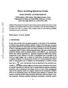
Different choices for ρ may produce inequivalent codes. Choosing ρ corresponds to choosing an encoding method for C2 . For example, if the second code is the [[1, 0, 1]] code with generator matrix [1], the new code has parameters [[n1 + 1, k1 , d1 ]], as in Theorem 6(a). A different [[n1 + 1, k, d1 ]] code is obtained if we take the second code to be the [[2, 1, 1]] code with generator matrix [11]. In particular, the second [[6, 1, 3]] code mentioned above may be obtained in this manner. Theorem 8 can be used to produce an analogue of concatenated codes in the quantum setting. If Q1 is an [[nm, k]] code such that the associated (nm, 2nm+k ) code has minimal nonzero weight d in each m-bit block, and Q2 is an [[n2 , m, d2 ]] code, then encoding each block of Q1 using Q2 (as in Theorem 8) produces an [[nn2 , k, dd2 ]] concatenated code. A particularly interesting example is obtained by concatenating the [[5, 1, 3]] Hamming code 4 (see Section 5) with � itself. We take� Q1 = Q2 , and let the associated linear (5, 2 ) code have 0 1 1 1 1 generator matrix . Then we obtain a [[25, 1, 9]] code for which the associated 1 0 1 ω ω ¯ (25, 224 ) and (25, 226 ) linear codes have the generator matrices shown in Fig. 1. Although the
Hamming code is pure, the concatenated code is not. The construction of quantum codes used in [17] and [72] can be restated in the present terminology (and slightly generalized): Theorem 9. Let C1 ⊆ C2 be binary linear codes. By taking C = ωC1 + ω ¯ C2⊥ in Theorem 2 we obtain an [[n, k2 − k1 , d]] code, where d = min{dist(C2 \ C1 ), dist(C1⊥ \ C2⊥ )}. Proof.
It is easily verified that C is additive and that C ⊆ C ⊥ = ω ¯ C1⊥ + ωC2 .
2
Another construction based on binary codes due to Gottesman [36] can be generalized as follows. Theorem 10. Let Sm be the classical binary simplex code of length n = 2m − 1, dimension m and minimal distance 2m−1 (Chapter 14 of [54]). Let f be any fixed-point-free automorphism 15
Figure 1: Generator matrices for a (25, 224 ) linear code (above the line) and its dual, a (25, 226 ) linear code (all rows), corresponding to a [[25, 1, 9]] quantum code. 000 0 0 000 0 0 000 0 0 00 0 0 0 01 1 1 1 000 0 0 000 0 0 000 0 0 00 0 0 0 10 1 ωω ¯ 000 0 0 000 0 0 000 0 0 01 1 1 1 00 0 0 0 000 0 0 000 0 0 000 0 0 10 1 ωω ¯ 00 0 0 0 000 0 0 000 0 0 011 1 1 00 0 0 0 00 0 0 0 000 0 0 000 0 0 101ωω ¯ 0 0 0 0 0 0 0 0 0 0 000 0 0 011 1 1 000 0 0 00 0 0 0 00 0 0 0 ¯ 000 0 0 00 0 0 0 00 0 0 0 000 0 0 101ωω 011 1 1 000 0 0 000 0 0 00 0 0 0 00 0 0 0 101ωω ¯ 000 0 0 000 0 0 00 0 0 0 00 0 0 0 000 0 0 001ω ¯ ω001ω ¯ ω00 1 ω ¯ ω00 1 ω ¯ω 001ω ¯ ω000 0 0 001ω ¯ ω00ω 1 ω ¯ 00ω ¯ω1 000 0 0 000 0 0 001ω ¯ ω00ω ¯ ω 1 00ω 1 ω ¯ of Sm and let Gm be the (2m , 2m+2 ) additive code generated by the vectors u + ωf (u), u ∈ Sm ,
with a 0 appended, together with the vectors 11 . . . 1, ωω . . . ω of length 2m . This yields a [[2m , 2m − m − 2, 3]] quantum code. We omit the proof. We can show that Gm has the following properties (again, to save space, the proofs are omitted). (i) For any choice of f , Gm has weight enumerator m
m−2
x2 + 4(2m − 1)x2
m−2
y 3.2
m
+ 3y 2
.
(ii) The vectors of weight 2m generate a subcode of dimension 2. ′ using f ′ . Then G ′ is (iii) Suppose Gm is constructed using the automorphism f , and Gm m
equivalent to Gm if and only if f ′ is conjugate under Aut(Sm ) to one of {f, 1 − f, 1/f, 1 − 1/f, 1/(1 − f ), f /(1 − f )} .
(9)
(iv) The automorphism group of Gm has a normal subgroup H which is a semidirect product of the centralizer of f in Aut(Sm ) with Sm , the index [Aut(Gm ) : H] being the number of elements of (9) that are conjugate to f . (v) Gm is linear precisely when f satisfies f 2 + f + 1 = 0. 16
Before giving some examples, we remark that Aut(Sm ) is isomorphic to the general linear group GLm (2), and conjugacy classes of GLm (2) are determined by their elementary divisors. So the most convenient way to specify f is by listing its elementary divisors. For m = 3, there is a unique choice for f , with elementary divisor x3 + x + 1, and so there is a unique G3 , with parameters [[8, 3, 3]]. Then Aut(G3 ) has order 168, and is a semidirect product of a cyclic group C3 with the general affine group GA1 (8). For m = 4 there are three distinct codes G4 , with parameters [[16, 10, 3]]. The corresponding elementary divisors for f are: (a) x2 + x + 1 (twice). This produces a linear code, with |Aut(G4 )| = 17280. (In general
the code is linear precisely when all the elementary divisors are equal to x2 + x + 1.) (b) (x2 + x + 1)2 , with |Aut(G4 )| = 1152. (c) x4 + x + 1, with |Aut(G4 )| = 480.
For m = 5 there are two distinct G5 codes, with parameters [[32, 25, 3]]. The corresponding elementary divisors are (a) x3 + x + 1 and x2 + x + 1, with |Aut(G5 )| = 2016. (b) x5 + x2 + 1, with |Aut(G5 )| = 992.
Gottesman [38] used just a single f , which 0 1 0 0 0 1 · · 0 0 0 1 1 1
he took to be (if m is even) 0 ··· 0 0 ··· 0 · ··· 0 ··· 1 1 ··· 1
while if m is odd the first row is complemented. Gottesman’s codes correspond to those labeled (c) (for m = 4) and (b) (for m = 5). The codes in Theorem 10 can be extended. Theorem 11. For m ≥ 2, there exists an [[n, n − m − 2, 3]] code, where n is m/2
X
(m−1)/2 2i
2
X
(m even),
i=0
Sketch of proof.
22i+1 (m odd) .
i=1
The corresponding (n, 2m+2 ) additive code C (say) has weight enumerator m
m
xn + (2m+2 − 1)xn−2 y 2
(m even)
or m +2
xn + (2m+2 − 2m )xn−2
m −2
y2
m
m
+ (2m − 1)xn−2 y 2
17
(m odd) .
We take C2 and C3 to be the additive codes corresponding to the [[5, 1, 3]] and [[8, 3, 3]] codes ′ be the subcode already mentioned. For m > 3, let Gm be as in Theorem 10, and let Gm
consisting of the weight 2m codewords in Gm . Finally, let φ be any isomorphism between Cm−2
′ (note that both are spaces of dimension m). Define a new code C to consist of and Gm /Gm m ′ . A simple counting argument verifies all vectors v1 v2 , where v1 ∈ Cm−2 and φ(v1 ) = v2 + Gm ⊥ has that Cm has the claimed weight distribution. By applying Theorem 5 we find that Cm
2
minimal distance 3. Theorem 11 was independently discovered by Gottesman [38].
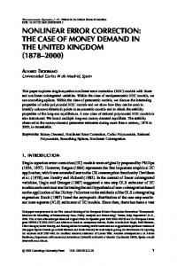
The resulting codes, like those constructed in Theorem 10, are pure and additive but in general are not linear. For even m we obtain the Hamming codes of Section 5 as well as nonlinear codes with the same parameters. For odd m we obtain [[8, 3, 3]], [[40, 33, 3]], [[168, 159, 3]], . . . codes. A generator matrix for the (40, 27 ) additive code corresponding to a [[40, 33, 3]] code is shown in Fig. 2. Figure 2: Generator matrix for (40, 27 ) additive code, producing a [[40, 33, 3]] quantum code.
0000000011111111111111111111111111111111 0 0 0 0 0 0 0 0ωωωωωωωωωωωωωωωωωωωωωωωωωωωωωωωω 0 0 1ω ¯ ωω ω ¯ 1ω 0 1 0 1 ω ¯ ωωω ¯ 1 0 1 0ωω ¯ 1 0ω ω ¯ ωω ¯ 1 0 0 1ω ¯ ωω ¯ω 0 1ω ¯ 0 1ωω 1 0 ω ¯ω ¯ 0ω 0 0ω 0ω ω ¯ 1ω ¯ 1 1ω ¯ 1ω ¯ω ¯ 1ω ¯ 1 1ω ¯ 1ω ¯ ω 0ω 0 0ω 0ωω 0ω 0 ω ¯ 1ω ¯ 1ω 0 1 1 0 0 1 1ωω ω ¯ω ¯ ωω ω ¯ω ¯ 0 0 1 1 0 0 1 1ωω ω ¯ω ¯ ωω ω ¯ω ¯ 0 1 0ω 0ω ω ¯ 1ω ¯ 0 0 0ωωωω 1 1 1 1 ω ¯ω ¯ω ¯ω ¯ 0 0 0 0ωωωω 1 1 1 1 ω ¯ω ¯ω ¯ω ¯ 0
ω 0ω 1 ω ¯ 1ω ¯ 0 0 0 0 1 1 1 1 0 0 0 0 1 1 1 1ωωωω ω ¯ω ¯ω ¯ω ¯ ωωωωω ¯ω ¯ω ¯ω ¯0
The “u|u + v” construction for binary codes ([54], page 76) has an analogue for quantum codes. Theorem 12. Suppose there is a pure [[n, k1 , d1 ]] code with associated (n, 2n−k1 ) additive code C1 , and a pure [[n, k2 , d2 ]] code with associated code C2 , such that C1 ⊆ C2 . Then there exists a pure [[2n, k1 − k2 , d]] code, where d = min{2d1 , δ}, δ = dist(C2 ). Proof.
Take C to be the (2n, 22n−k1 +k2 ) additive code consisting of the vectors u|u + v,
u ∈ C2⊥ , v ∈ C1 , where the bar denotes concatenation. Then C ⊥ = {u|u + v : u ∈ C1⊥ , v ∈ C2 } has minimal distance min{2d1 , δ}, by Theorem 33 of [54], Chapter 1.
2
For example, by combining the [[14, 8, 3]] and [[14, 0, 6]] codes shown in Table II of the next section we obtain a [[28, 8, 6]] code. 18
Concerning the structure of additive but nonlinear codes, it is pointless to simply add one generator to a linear code. For if D is an (n, 2n+k ) linear code, and D ′ = hD, vi is an
(n, 2n+k+1 ) additive code with minimal distance d, then it is easy to show that the linear code D ′′ = hD, v, ωvi also has minimal distance d. We end this section by listing some trivial codes. An [[n, k, 1]] code exists for all 0 ≤ k ≤ n, n ≥ 1. An [[n, k, 2]] code exists provided 0 ≤ k ≤ n − 2, if n ≥ 2 is even, or provided 0 ≤ k ≤ n − 3 if n ≥ 3 is odd.
5. Cyclic and related codes An (n, 2k ) additive code C is constacyclic if there is a constant κ (which in our case will be 1, ω or ω ¯ ) such that (u0 , u1 , . . . , un−1 ) ∈ C implies (κun−1 , u0 , u1 , . . . , un−2 ) ∈ C. If κ = 1 the code is cyclic. Besides these standard terms from the classical theory, we also need a new concept: if (u0 , u1 , . . . , un−1 ) ∈ C implies (¯ un−1 , u0 , u1 , . . . , un−2 ) ∈ C, the code will be called conjucyclic. We begin with linear codes. If vectors are represented by polynomials in the natural way, a linear constacyclic code is represented by an ideal in the ring of polynomials modulo xn − κ ([54], [49]). The latter is a principal ideal ring, so the code consists simply of all multiples of a single generator polynomial g(x), which must divide xn − κ. We assume n is odd. Theorem 13. A linear cyclic or constacyclic code with generator polynomial g(x) is selforthogonal if and only if g(x)g† (x) ≡ 0 (mod xn − κ) , where if g(x) =
Pn−1 j=0
gj xj , n−1 X
g† (x) = κ¯ g0 +
g¯n−j xj .
(10)
j=1
We omit the elementary proof (cf. [15]). Note that
g† (x) ≡ κg(x−1 ) (mod xn − κ) . The † operation induces an involution on factors of xn − κ, so we can write xn − κ =
Y i
pi (x)
Y j
19
(qj (x)qj† (x)) ,
(11)
where the pi , qj and qj† are all distinct and p†i = pi . Then a divisor g(x) of xn − κ generates a self-orthogonal linear constacyclic code if and only if g(x) is divisible by each of the pi ’s and by at least one from each qj , qj† pair. Example.
The classical Hamming code H over GF (4) has length n = (4m − 1)/3, contains
4n−m codewords and has minimal distance 3, for m ≥ 1 [54], [52]. The dual code C = H ⊥ is a self-orthogonal linear code, and the corresponding quantum code has parameters [[n, n−2m, 3]], where n = (4m − 1)/3. C and H are cyclic if m is even, constacyclic if m is odd. For example
when m = 2 we can take H to have generator polynomial g(x) = x2 + ωx + 1, a divisor of
x5 − 1, and when m = 3 we take g(x) = x3 + x2 + x + ω, a divisor of x21 − ω. These codes meet the sphere-packing bound (14) (see Section 7) with equality. The smallest Hamming code, a [[5, 1, 3]] code, was independently discovered in the present context by [5] and [50]. See also [16]. Hamming codes correct single errors. In the classical theory the generalizations of Hamming codes that correct multiple errors are known as BCH codes [54]. A similar generalization yields multiple-error correcting quantum codes. Rather than giving a complete analysis of these codes, which involves a number of messy details, we simply outline the construction and give some examples. These quantum BCH codes may be cyclic or constacyclic. In the cyclic case we let ξ be a primitive n-th root of unity in some extension field of GF (4), Q and write each factor qj in (11) as qj (x) = s∈Sj (x − ξ s ), the zero set Sj being a cyclotomic
coset modulo n under multiplication by 4 (see [54], Chap. 7). The zero set associated with qj†
is then −2Sj . We choose a minimal subset of the qj ’s subject to the conditions that (a) there is an arithmetic progression of length d − 1 in the union of its zero sets, for which the step size is
relatively prime to n, and (b) if qj is chosen, qj† is not. Let B be the cyclic code whose generator
polynomial is the product of the qj ’s. Then (a) guarantees that B has minimal distance at least d and (b) guarantees that B ⊃ B ⊥ . In this way we obtain a quantum error-correcting code with parameters [[n, k, d]], where k = n − 2 deg g. A similar construction works in the constacyclic case, only now we choose ξ to be a primitive (3n)-th root of unity. In the special case when n = (4m − 1)/3, most of the qj have degree m, and we obtain a
20
sequence of cyclic or constacyclic codes which provided m is at least 4, begins [[n, n − 2m, 3]], [[n, n − 4m, 4]], [[n, n − 6m, 5]], [[n, n − 8m, 7]], . . . . For example when m = 4 we obtain [[85, 77, 3]], [[85, 69, 4]], [[85, 61, 5]] and [[85, 53, 7]] codes. We now discuss additive (but not necessarily linear) codes. Note that an additive constacyclic code (with κ = ω or ω ¯ ) is necessarily linear. Theorem 14. (a) Any (n, 2k ) additive cyclic code C has two generators, and can be represented as hωp(x) + q(x), r(x)i, where p(x), q(x), r(x) are binary polynomials, p(x) and r(x)
divide xn − 1 (mod 2), r(x) divides q(x)(xn − 1)/p(x) (mod 2), and k = 2n − deg p − deg r.
(b) If hωp′ (x) + q ′ (x), r ′ (x)i is another such representation, then p′ (x) = p(x), r ′ (x) = r(x) and q ′ (x) ≡ q(x) (mod r(x)). (c) C is self-orthogonal if and only if p(x)r(xn−1 ) ≡ p(xn−1 )r(x) ≡ 0 (mod xn − 1) , p(x)q(xn−1 ) ≡ p(xn−1 )q(x) (mod xn − 1) . Proof.
(a) Consider the map Tr : C → Z2[x]/(xn − 1) obtained by taking traces
componentwise. The kernel of this map is a binary cyclic code, so can be represented uniquely as hr(x)i, where r(x) divides xn − 1. The image of the map is similarly a binary cyclic code hp(x)i. The original code is generated by r(x) and some inverse image of p(x), say ωp(x)+q(x).
Finally, if r(x) did not divide q(x)(xn − 1)/p(x), then ((xn − 1)/p(x))(ωp(x) + q(x)) would be
a binary vector of C not in hr(x)i, a contradiction. We omit the proof of (b). (c) One readily verifies that the inner product of the vectors corresponding to ωf (x) + g(x) and ωh(x) + i(x) is given by the constant coefficient of f (x)i(xn−1 ) + g(x)h(xn−1 ) (mod xn − 1) . But then the inner product of the vectors corresponding to ωf (x) + g(x) and xm (ωh(x) + i(x)) is given by the coefficient of xm in f (x)i(xn−1 ) + g(x)h(xn−1 ). The result follows immediately.
2 We remark without giving a proof that if C is self-orthogonal we may assume that q(x) satisfies q(xn−1 ) =
π(x) σ(x)(xn − 1) + , p(x) p(x)
21
(12)
and r(x) divides q(x)(xn −1)/p(x), where π(x) ≡ π(xn−1 ) ( mod xn −1), π(x) ≡ 0 ( mod p(x)), and deg σ < deg r + deg p − n. This makes it possible to search through all self-orthogonal
additive cyclic codes of a given dimension: r(x) ranges over all divisors of xn − 1, p(x) ranges over all divisors of (xn − 1)/gcd{r(xn−1 ), xn − 1} of the appropriate degree, and finally all
choices for π(x) and σ(x) must be considered. Table I lists some additive cyclic codes that were found in this way. Table I: Cyclic codes. Parameters
Generators for additive code
[[15, 0, 6]]
ω 1 1 0 1 0 1 0 0101011
[[21, 0, 8]]
ω ¯ω ¯ 1ω 0 0 1 1 1101011011000 , 101110010111001011100
[[21, 5, 6]]
ω 0ω ¯ω ¯ ωω ¯ω ¯ 0ω100100001001 , 101110010111001011100
[[23, 0, 8]]
ω 0 1 0 1 1 1 1 000000001111010
[[23, 12, 4]]
ω ¯ω ¯ ωω ¯ω 1 1ω ¯ 11ω1ω1011000000
[[25, 0, 8]]
1 1 1 0 1 0ω 0 10111000000000000
Theorem 15. Let C be an (n, 2k ) additive conjucyclic code, and form the binary code C ′ = {Tr(ωu)|Tr(¯ ω u) : u ∈ C} , when the trace is applied componentwise and the bar denotes concatenation. Then C ′ is a binary cyclic code of length 2n, which is self-orthogonal if and only if C is self-orthogonal. We omit the proof. Note that C ′ determines C, since ωTr(ωu) + ω ¯ Tr(¯ ω u) = u . Theorem 15 makes it possible to search for codes of this type. So far no record codes have been found. We now return to linear codes. A quasicyclic code is a code of length n = ab on which the group acts as a cycles of length b. T. A. Gulliver of Carleton University (Canada) and the University of Canterbury (New Zealand) has extensively studied quasicyclic codes over small fields [39]. The last five examples in Table II were found by him. Double parentheses indicate the cycles of the permutation that is to be applied.
22
Table II: Linear quasicyclic codes. Parameters
Generator
[[14, 0, 6]]
((1000000)) ((¯ ω 1¯ ω ω00ω))
[[14, 2, 5]]
((1000001)) ((1ω101ω1))
[[14, 8, 3]]
((1011100)) ((1¯ ω ωω10¯ ω ))
[[15, 5, 4]]
((10000)) ((11¯ ω 00)) ((11ωω0))
[[18, 6, 5]]
((110000)) ((101¯ ω 00)) ((11ω1ω0))
[[20, 10, 4]]
((10000)) ((1¯ ω 100)) ((1111ω)) ((11¯ ωωω ¯ ))
[[25, 15, 4]]
((10000)) ((1ω1ω0)) (0101¯ ω )) ((1ω ω ¯ ω1)) ((10ωω0))
[[28, 14, 5]]
((ωω ω ¯ 1000)) ((¯ ω 0¯ ω 1000)) ((1¯ ωω ¯ 1ω ω ¯ 0)) ((¯ ωωω ¯ ωω00))
[[30, 20, 4]]
((11100)) ((10ω00)) ((11¯ ω ω0)) ((1ω1ω ω ¯ )) ((10ω10)) ((1ω100))
[[40, 30, 4]]
((001ωω)) ((011ω1)) ((0010¯ ω )) ((001ω1)) ((00101)) ((1ω1ω ω ¯ )) ((111¯ ω ω)) ((01ω1¯ ω ))
6. Self-dual codes In this section we study [[n, 0, d]] quantum-error-correcting codes and their associated (n, 2n ) self-dual codes C. These codes are of interest in their own right — for instance, the unique [[2, 0, 2]] code corresponds to the quantum state
√1 (|01i 2
− |10i), that is, an EPR pair.
They are also important for constructing [[n, k, d]] codes with k > 0, as we will see in Section 8. We begin with some properties of weight enumerators of self-dual codes. Theorem 16. (a) The weight enumerator of a self-dual code is fixed under the transformation � � � �� � x 1 1 x 3 replace by , (13) y 2 1 −1 y and is therefore a polynomial in x + y and x2 + 3y 2 . (b) The minimal distance of a self-dual code of length n is ≤ [n/2] + 1. Proof.
(a) (13) follows from Theorem 5, and the proof of the second assertion is parallel to
that of Theorem 13 of [53]. (b) Parallel to the proof of Corollary 3 of [55].
2
(The result in (b) has since been improved — see Section 9.) Theorem 17. (a) The weight enumerator of an even self-dual code is a polynomial in x2 +3y 2 and y 2 (x2 −y 2 )2 . (b) The minimal distance of an even self-dual code of length n is ≤ 2[n/6]+2. 23
Proof.
(a) This is an immediate consequence of Theorem 13 of [53]. (b) From Corollary 15
of [53].
2
In view of the importance of doubly-even self-dual codes in binary coding theory, we also note the following result. Theorem 18. If there is an integer constant c > 1 such that the weight of every vector in a self-dual code is divisible by c, then c = 2. Proof.
The proof of the Gleason-Prange theorem for classical self-dual codes over an alphabet
2
of size 4 as given in [71] applies unchanged.
(Note that applying the Calderbank-Shor-Steane construction (cf. Theorem 9) to a doublyeven binary code does not give a code with weights divisible by 4. For example, the GF (4)-span of the Golay code of length 24 contains words of weight 14.) It is possible to give a complete enumeration of all self-dual codes of modest length, following the methods of [53] and [24]. Theorem 19. (a) The total number of self-dual codes of length n is Qn j X 1 j=1 (2 + 1) (b) = , |Aut(C)| 6n n!
Qn
j j=1 (2
+ 1).
where the sum is over all inequivalent self-dual codes C of length n. Proof.
(a) Parallel to that of Theorem 19 of [53]. (b) From (a) and (6).
2
Let dn be the (n, 2n−1 ) code spanned by all even-weight binary vectors of length n, n ≥ 2,
and let d+ n = hdn , ωω . . . ωi.
Theorem 20. Suppose C is a self-orthogonal additive code, in which no coordinate is identically zero, and which is generated by words of weight 2. Then C is equivalent to a direct sum + d+ 2 ⊕ . . . ⊕ d2 ⊕ di ⊕ dj ⊕ dk ⊕ . . . , i, j, k ≥ 2.
Proof.
Analogous to that of Theorem 4 of [24].
2
With the help of Theorems 19 and 20 we find that the numbers tn (respectively in ) of inequivalent (respectively inequivalent indecomposable) self-dual codes of length n for n ≤ 5
24
are
n 1 2 3 4 5 tn 1 2 3 6 11 in 1 1 1 2 4
This enumeration could be extended to larger values of n without too much difficulty. The indecomposable codes mentioned in the above table are the trivial code c1 , the codes ¯ i, the length 5 codes d+ n for n ≥ 2, the length 4 code h1100, 0011, ωωωω, 01ω ω h11000, 00110, 00101, 01ωωω, ωω001i and h11000, 00110, 10101, ωω00ω, 00ωωωi , and a (5, 25 ) d = 3 code obtained from the hexacode (see Section 8) using Theorem 6. We have also investigated the highest achievable minimal distance of any self-dual code of length n, or equivalently of any [[n, 0, d]] quantum-error-correcting code. The results are shown in the k = 0 column of the main table (Section 8). Of course in view of Theorem 6(c) this also gives bounds on the minimal distance of any pure [[n, k, d]] code. We see from that table that the bound in Theorem 17 for even self-dual codes is met with equality at lengths 2, 4, . . . , 22, 28 and 30. In all but one of those cases the code can be taken to be a classical self-dual linear code over GF (4). The exception is at length 12, where although no classical self-dual codes exists with minimal distance 6 [24], there is a unique additive code. This is the (12, 212 ) d = 6 additive code having generator matrix 000000111111 0 0 0 0 0 0ωωωωωω 1 1 1 1 1 1 0 0 0 0 0 0 ωωωωωω 0 0 0 0 0 0 0 0 0 1ω ω ¯ 0 0 0 1ω ω ¯ ¯ 1 0 0 0ω ω ¯ 1 0 0 0ω ω , ¯ω 0 0 0 1ω ¯ω 0 0 0 1ω ω 1ω ¯ 0 0 0ω 1 ω ¯ 0 0 0 0 0 0 1ω ¯ ωω ω ¯ 1 0 0 0 0 0 0ω 1 ω ¯ 1ω ω ¯ 0 0 0 1ω ω ¯ 0 0 0 0 0 0ω ¯ω 1 ω ¯ 1ω 0 0 0 0 0 0 1 ω ¯ω which we will call the dodecacode. This code is equivalent to the cyclic code with generator ω10100100101. It has weight distribution A0 = 1, A6 = 396, A8 = 1485, A10 = 1980, A12 = 234, and its automorphism group has order 648 and acts transitively on the coordinates. 25
There is an interesting open question concerning length 24. There exists a (24, 224 ) d = 8 classical code over GF (2), the Golay code, and at least two (24, 312 ) d = 9 classical codes over GF (3), all meeting the analogous bounds to Theorem 17(b) [54]. It is known [51] that there is no (24, 412 ) d = 10 classical code over GF (4), but the possibility of a (24, 224 ) d = 10 additive self-dual code remains open. Linear programming shows that if such a code exists then it must be even. However, all our attempts so far to construct this code have failed, so it may not exist.
7. Linear programming and other bounds Gottesman [36] showed that any nondegenerate [[n, k, 2t + 1]] code must satisfy the spherepacking bound t X j=0
� � n 3 ≤ 2n−k . j j
(14)
Knill and Laflamme [47] have shown that any (pure or impure) code must satisfy the following version of the Singleton bound (cf. [54]): n ≥ 4e + k,
(15)
where e = ⌊(d − 1)/2⌋ is the number of errors correctable by the code. In this section we first establish a linear programming bound which applies to all [[n, k, d]] codes, and then give a slightly stronger version of the Singleton bound for pure codes. Suppose an [[n, k, d]] code exists, let C be the corresponding (n, 2n−k ) code over GF (4) and let C ⊥ , an (n, 2n+k ) code, be its dual (see Theorem 2). Let A0 , . . . , An and A′0 , . . . , A′n be the weight distributions of C and C ⊥ respectively. In view of Theorem 6(e), we may assume that A1 = 0. (Only minor modifications to Theorem 21 are required if this assumption is not made.) The Krawtchouk polynomials appropriate for studying a code of length n over GF (4) will be denoted by Pj (x, n) =
j X
s j−s
(−1) 3
s=0
� �� � x n−x , s j−s
for j = 0, . . . , n (see Chapter 6 of [54]). Theorem 21. If an [[n, k, d]] quantum-error-correcting code exists such that the associated (n, 2n−k ) code C contains no vectors of weight 1, then there is a solution to the following set 26
of linear equations and inequalities: A0 = 1, A1 = 0, Aj ≥ 0 (2 ≤ j ≤ n) ,
(16)
A0 + A1 + · · · + An = 2n−k , n 1 X ′ Pj (r, n)Ar (0 ≤ j ≤ n) , Aj = n−k 2
(17) (18)
r=0
Aj = A′j (0 ≤ j ≤ d − 1), Aj ≤ A′j (d ≤ j ≤ n) , X A2j = 2n−k−1 or 2n−k ,
(19) (20)
j≥0
1 2n−k−1
n X r=0
Pj (2r, n)A2r ≥ A′j (0 ≤ j ≤ n) .
(21)
(If the second possibility obtains in (20), (21) just says that 2A′j ≥ A′j and can be omitted.) Proof.
(18) is a consequence of Theorem 5, and (19) follows from the facts that C ⊂ C ⊥
and any vectors in C ⊥ of weights between 1 and d − 1 inclusive must also be in C. From (7), the even weight vectors in C form an additive subcode C ′ , which is either half or all of C; (20) then follows. If C ′ is half of C, then C ′ ⊂ C ⊂ C ⊥ ⊂ (C ′ )⊥ , which yields (21). The other
2
constraints are clear.
A more compact statement of the linear programming bound may be obtained by rephrasing Theorem 21 in terms of weight enumerators. Theorem 22. If an [[n, k, d]] quantum-error-correcting code exists then there are homogeneous polynomials W (x, y), W ⊥ (x, y) and S(x, y) of degree n such that the following conditions hold: W (1, 0) = W ⊥ (1, 0) = 1 , � � x + 3y x − y ⊥ k , W (x, y) = 2 W , 2 2 � � x + 3y y − x , , S(x, y) = 2k W 2 2 W ⊥ (1, y) − W (1, y) = O(y d ) ,
(22) (23) (24) (25)
and W (x, y), W ⊥ (x, y) − W (x, y), S(x, y) ≥ 0 , where P (x, y) ≥ 0 indicates that the coefficients of P (x, y) are nonnegative.
27
(26)
Proof.
Take W (x, y) to be the weight enumerator of C and W ⊥ (x, y) to be the weight
enumerator of C ⊥ . S(x, y) is the shadow enumerator (by analogy with [25]) and is nonnegative
2
by Eq. (21). We have implemented Theorems 21 and 22 on the computer in two different ways.
(i) We attempt to minimize A1 + · · · + Ad−1 subject to (16)–(21) using an optimization program such as CPLEX [27] or CONOPT [32]. The AMPL language [35] makes it easy to formulate such problems and to switch from one package to another. If all goes well, the program either finds a solution (which may lead to additional discoveries about the code, such as that there must exist a vector of a particular weight), or else reports that no feasible solution exists, in which case we can conclude that no [[n, k, d]] code exists. Unfortunately, for values of n around 30, the coefficients may grow too large for the problems to be handled using double precision arithmetic, and the results cannot be trusted.3 (ii) Alternatively, using a symbolic manipulation program such as MAPLE [18], we may ask directly if there is a feasible solution to (16)–(21) or to (22)–(26) (the latter being easier to implement). Since the calculations are performed in exact arithmetic, the answers are (presumably) completely reliable. On the other hand the calculations are much slower than when floating point arithmetic is used. Most of the upper bounds in the main table were independently calculated using both methods. When investigating the possible existence of a pure [[n, k, d]] code, we may set A2 through Ad−1 equal to 0. In all cases within the range of table III below, this had no effect; that is, the LP bound for pure codes was the same as that for impure codes. We handle (20) by running the problem twice, once for each choice of the right-hand side. For example, using Theorem 21 we find that there are no [[n, 1, 5]] codes of length n ≤ 10 for which C has A1 = 0. From Theorem 6 we conclude that no [[n, 1, 5]] code of any type exists with n ≤ 10. On the other hand an [[11, 1, 5]] code does exist — see the following section. Additional constraints can be included in Theorem 21 to reflect special knowledge about particular codes, or to attempt to narrow the range of a particular Ai . Many variations are the basic argument are possible, as illustrated in the following examples. (i) No [[13, 0, 6]] code exists. Let C be a (13, 213 ) additive code with d ≥ 5, and let C ′ be 3
It is hoped that the multiple precision linear programming package being developed by David Applegate of Rice University will soon remove this difficulty.
28
its even subcode. The linear constraints in Theorem 21 enable us to express all the unknowns in terms of A5 and A6 . The condition that the weight distribution of (C ′ )⊥ be integral implies certain congruence conditions on A5 and A6 , from which it is possible to eliminate A6 . The resulting congruence implies A5 ≡ 1 (mod 2). In particular A5 6= 0, and so d = 5.
(ii) No [[18, 12, 3]] code exists. Consider the (18, 26 ) additive code C. Linear programming
shows that C must contain a vector of weight 12, which without loss of generality we may take to be u0 = 06 112 . We define the refined weight enumerator of C with respect to u0 to be RC (x0 , x1 , y0 , y1 , y2 ) =
X
6−a(u) a(u) 12−b(u)−c(u) b(u) c(u) x1 y 0 y1 y2
x0
,
u∈C
where a(u) is the weight of u in the first 6 coordinates, and b(u) (resp. c(u)) is the number of 1’s (resp. ω’s or ω ¯ ’s) in u in the last 12 coordinates. The conditions on C imply that c(u) ≡ 0 (mod 2), (a(u + u0 ), b(u + u0 ), c(u + u0 )) = (a(u), 12 − b(u) − c(u), c(u)) , and RC ⊥ =
1 RC (x0 + 3x1 , x0 − x1 , y0 + y1 + 2y2 , y0 + y1 − 2y2 , y0 − y1 ) . |C|
By applying linear programming, we find that the weight distribution of C must be either A0 = 1, A12 = 9, A14 = 54 or A0 = 1, A12 = 1, A13 = 24, A14 = 30, A15 = 8. In either case, adding these constraints to the refined weight enumerator produces a linear program with no feasible solution. (iii) Similar arguments eliminate the parameters [[7, 0, 4]], [[15, 4, 5]], [[15, 7, 4]], [[16, 8, 4]], [[19, 0, 8]], [[19, 3, 3]], [[22, 14, 4]] and [[25, 0, 10]]. In the remainder of this section we briefly discuss another version of the Singleton bound (cf. (15)): Theorem 23. If a pure [[n, k, d]] code exists then k ≤ n − 2d + 2. Proof.
The associated code C ⊥ is then an additive (n, 2n+k ) code with minimal distance d.
From Theorem 15 of [28], we have 2n+k ≤ 4n−d+1 , which implies k ≤ n − 2d + 2.
2
If d is odd this coincides with the Knill and Laflamme bound (15), but is slightly stronger if d is even. 29
We have determined all codes that meet this bound — these are analogues of the classical MDS codes (cf. Chapter 11 of [54]). Since the results are somewhat disappointing we simply state the answer and omit the rather lengthy proof. Theorem 24. A pure [[n, n − 2d + 2, d]] code has parameters [[n, n, 1]] (n ≥ 1), [[n, n − 2, 2]] (n even ≥ 2), [[5, 1, 3]] or [[6, 0, 4]]. Up to equivalence there is a unique code in each case. Even allowing k = n − 2d + 1 does not appear to lead to any new codes. Further analysis shows that any pure [[n, n − 2d + 1, d]] code has parameters [[n, n − 1, 1]] (n ≥ 1), [[n, n − 3, 2]] (n ≥ 3), [[5, 0, 3]] or [[8, 3, 3]].
8. A table of quantum-error-correcting codes Table III, obtained by combining the best upper and lower bounds given in the previous sections, shows our present state of knowledge about the highest minimal distance d in any [[n, k, d]] code of length n ≤ 30. Table III about here
Notes on Table III When the exact value of d is not known, the lower and upper bounds are separated by a dash. All unmarked upper bounds in the table come from the linear programming bound of Theorem 21. (A few of these bounds can also be obtained from Eq. (14) or from Theorem 16.) Unmarked lower bounds are from Theorem 6. Note in particular that, except in the k = 0 column, once a particular value of d has been achieved, the same value holds for all lower entries in the same column using Theorem 6(a). α. A code meeting this upper bound must be impure (this follows from integer programming by an argument similar to that used in Section 7 to show that no [[13, 0, 6]] code exists). β. A special upper bound given in Section 7. These bounds do not apply to nonadditive codes, for which the upper bound must be increased by 1. γ. This is the unique other entry in the table (besides those marked ‘β’) where the known upper bound for nonadditive codes is different from the bound for additive codes: if we 30
omit (21) (which says that the code is either odd or even) from the linear program, the bound increases by 1. In all other entries in the table, condition (21) is superfluous. However, we will be surprised if a ((19, 28 , 5)) nonadditive code exists. Most of the following lower bounds are specified by giving the associated (n, 2n−k ) additive code. a. The hexacode, a (6, 26 ) d = 4 classical code that can be taken to be the GF (4) span of h001111, 0101ω ω ¯ , 1001¯ ω ωi (see Chapter 3 of [26]). Aut(h6 ) = 3.S6 , of order 2160. b. A classical self-dual code over GF (4) — see [53], [24]. c. A cyclic code, see Table I. d. A [[25, 1, 9]] code obtained by concatenating the [[5, 1, 3]] Hamming code with itself (Fig. 1 of Section 4). e. The dodecacode defined in Section 6. f. An [[8, 3, 3]] code, discovered independently in [16], [36] and [73]. The (8, 25 ) additive code may be generated by vectors ((01ωω ω ¯ 1¯ ω ))0, 11111111, ωωωωωωωω (where the double parentheses mean that all cyclic shifts of the enclosed string are to be used). Exhaustive search shows that this code is unique. Another version is obtained from Theorem 10. The automorphism group has order 168, and is the semidirect product of a cyclic group of order 3 and the general affine group {x → ax + b : a, b, x ∈ GF (8), a 6= 0}. g. A quasicyclic code found by T. A. Gulliver — see Table II of Section 5. h. A Hamming code, see Section 5. i. Use the (12, 28 ) and (14, 28 ) linear codes with generator matrices 0000 0 0 11 1 1 1 1 0011 1 1 00 1 1 ωω 0101ωω ¯ 01 0 ω 1 ω 1001ω ¯ ω01ω 0 ω 1 and
0000 0 0 11 1 1 11 1 1 0011 1 1 00 0 0 11 1 1 0101ωω ¯ 01ωω ¯ 01ωω ¯ 1001ω ¯ ω01ω ¯ ω10ωω ¯
31
respectively. Their automorphism groups have orders 720 and 8064, and both act transitively on the coordinates. The first of these can be obtained from the u|u+v construction (c.f. Theorem 12) applied to the unique [[6, 4, 2]] and [[6, 0, 4]] codes. j. A [[17, 9, 4]] code, for which the corresponding (17, 28 ) d = 12 code C is a well-known linear code, a two-weight code of class TF3 [14]. The columns of the generator matrix of C represent the 17 points of an ovoid in P G(3, 4). Both C and C ⊥ are cyclic, a generator for C ⊥ being 1ω1ω1012 . The weight distribution of C is A0 = 1, A12 = 204, A16 = 51, and its automorphism group has order 48960. k. The [[16, 4, 5]] extended cyclic code spanned by (¯ ωω ¯ 0ω1ω111100111)0, together with vectors of all 1’s and all ω’s. s. By shortening one of the following codes using Theorem 7 or its additive analogue: the [[21, 15, 3]] or [[85, 77, 3]] Hamming codes (see Section 5), the [[32, 25, 3]] Gottesman code (Theorem 10), the [[40, 30, 4]] code given in Table II or the [[40, 33, 3]] code shown in Fig. 2. u. From the u|u + v construction (see Theorem 12). v. The following (17, 26 ) code with trivial automorphism group found by random search:
0 0 1 0ω ω ¯ ωω ¯ 1 1ω ω ¯ 0 0 1 1ω ¯ 0 0ω 1 0ω 0 ω ¯ω ¯ω ¯ 1 1ω ω ¯ω ¯ 1 1 0 1 0 0 1ω 1ωω ¯ω ¯ω ¯ 0ω ¯ 1ω 0 ω ¯ 0ω 0ωω 0 ω ¯ 1ω ¯ 1ω ω ¯ ω 1ωω 1 1 0 0ω ω ¯ 0 0 1ωω ω ¯ 1ω ¯ω 0ω ¯ 1 ω 0 0 1ω ¯ω ¯ω ¯ 0ω ¯ 0ω ¯ 1 0 1 1ω ω ¯
Comparison of the table with the existing tables [11] of classical codes over GF (4) reveals a number of entries where it may be possible to improve the lower bound by the use of linear codes. For example, classical linear [30, 18, 8] codes over GF (4) certainly exist. If such a code can be found which contains its dual, we would obtain a [[30, 6, 8]] quantum code.
32
Table III: Highest achievable minimal distance d in any [[n, k, d]] quantum-error-correcting code. The symbols are explained in the text. n\k
3 4 5 6 7 8 9 10 11 12 13 14 15 16 17 18 19 20 21 22 23 24 25 26 27 28 29 30
0
1
2 1 2 2 h3 3 a4 3α β s3 3 b4 s3 s3 4 b4 4 5 5 e6 5α 5β 5 b6 5 c6 5 b6 6 7 7 b8 7 β 7 7 b8 7 c8 7 b8 7−8 c8 − 9 7−9 b 8 − 10 8 − 9α c 8 − 9β d9 8 − 10 9 9 − 10 9 10 10 11 11 b 12 11α
2
3
4
1 1 2 1 1 2 1 1 2 2 2 2 2 2 s3 f3 2 s3 s3 2 s3 s3 4 s3 s3 4 i4 4 4 4 4 4 g5 4−5 4 g 4β 5 5 k5 6 5 6 5−6 5 6 5−6 5−6 6 5−6 5−6 6−7 5−7 5−6 6−7 6−7 6−7 6−8 6−7 6−7 6−8 6−8 6−7 6−8 6−8 6−8 7−8 7−8 7−8 8−9 8−9 8 9 9 8−9 10 9 8−9 10 9 − 10 8 − 9 10 9 − 10 8 − 10
33
5
6
7
1 1 1 2 2 2 s3 s3 3−4 4 4 4−5 4−5 5 5−6 5−6 c6 6−7 6−7 6−7 7−8 7−8 7−8 7−9 7−9 7−9
1 1 2 2 2 2 s3 s3 i4 4 4 4−5 g5 5 5−6 5−6 5−6 5−7 6−7 6−7 6−8 6−8 6−8 6−9 6−9
1 1 1 2 2 2 s3 s3 s 3β 3−4 4 4 4−5 4−5 c 5 − 6α 5−6 5−6 5−7 5−7 5−8 5−8 6−8 6−8 6−9
Table III cont. n\k
3 4 5 6 7 8 9 10 11 12 13 14 15 16 17 18 19 20 21 22 23 24 25 26 27 28 29 30
8
9
10
11
12
13
14
15
1 1 2 2 2 2 s3 s3 s 3β 4 4 4γ 4−5 4−5 4−6 4−6 4−6 4−7 4−7 4−8 u6 − 8 6−8 6−8
1 1 1 2 2 2 s3 s3 j4 4 4 4 4−5 4−5 4−6 4−6 4−6 4−7 5−7 5−8 5−8 5−8
1 1 2 2 2 2 s3 s3 s3 3−4 g4 4 4−5 4−5 4−6 4−6 4−6 4−7 5−7 5−7 5−8
1 1 1 2 2 2 v3 s3 s3 3−4 s4 4 4−5 4−5 4−6 4−6 4−6 5−7 5−7 5−7
1 1 2 2 2 2 2β s3 s3 3−4 s4 c4 4−5 4−5 4−6 4−6 5−6 5−6 5−7
1 1 1 2 2 2 2β s3 s3 3−4 s4 4 4−5 4−5 4−5 5−6 5−6 5−6
1 1 2 2 2 2 2 s3 s 3β 3−4 s4 4 4−5 4−5 g5 − 6 5−6 5−6
1 1 1 2 2 2 h3 s3 s3 3−4 g4 4 4−5 4−5 4−5 4−6
34
Table III cont. n\k
3 4 5 6 7 8 9 10 11 12 13 14 15 15 16 17 18 19 20 21 22 23 24 25 26 27 28 29 30
16
17
18
19
20
21
1 1 1 2 1 1 2 1 1 1 2 2 2 1 1 2 2 2 1 1 1 2 2 2 2 2 1 s3 2 2 2 2 1 s3 s3 2 2 2 2 s s 3 3 3−4 2 2 2 s4 s3 s3 3−4 2 2 s s s 4 3−4 2 4 3 3 s4 s3 s3 4 4 3−4 s3 4−5 4 4 3−4 3−4 g4 4−5 4−5 4 4 3−4
35
22 23
1 1 2 2 2 2 2 s3 s3
1 1 1 2 2 2 2 s3
9. Subsequent developments In the nearly two years since the manuscripts of [16] and the present paper were first circulated there have been a number of further developments. (i) While we showed in Section 2 that the Clifford group L suffices to encode additive codes, we did not give explicit recipes for doing so. Such recipes can now be found in Cleve and Gottesman [21]. (ii) The Cleve and Gottesman technique applies only to real (not complex) codes. However, it can be shown [58] that any additive code is equivalent to a real additive code (and any linear code is equivalent to a real linear code), so this is not a severe restriction. (iii) DiVincenzo and Shor [30] have shown how to correct errors in additive codes even when using imperfect computational gates. The techniques of Shor [66] for performing computations on encoded qubits using imperfect gates have been extended to general additive codes by Gottesman [37]. However, the most efficient methods currently known for fault-tolerant computation [2], [44], [48], [75] use only Calderbank-Shor-Steane codes (cf. Theorem 9). (iv) It turns out that the proofs of the lower bounds on the capacity of quantum channels given in Bennett et al. [4], [5] and DiVincenzo, Shor and Smolin [31] can be restated in terms of additive codes. In particular, this implies that these bounds can be attained using additive codes. (v) Cleve [20] has found a way to apply asymptotic upper bounds for classical binary codes to additive codes. (vi) Steane [74] has extended Gottesman’s [36] construction (compare Theorem 10) to obtain quantum analogues of Reed-Muller codes. The smallest of these new codes has parameters [[32, 10, 6]]. (vii) The upper bounds in the column headed ‘k = 0’ in Table III (with the exception of the entries marked ‘β’) have an obvious pattern with period 6. Further investigation of this pattern has led to an n/3 bound for quantum codes (cf. Theorem 17) [58] and an analogous n/6 bound for classical singly-even binary self-dual codes [57]. (viii) The main construction in this paper (described in Section 2) can be generalized to primes greater than 2. Some preliminary work along these lines has been done in [2], [45], [46], [60].
36
(ix) There are analogues of parts (a)–(c) of Theorem 6 for nonadditive codes. Parts (a) and (c) are trivial, while (b) now asserts that if a pure ((n, K, d)) codes exists with n ≥ 2 then an ((n − 1, 2K, d − 1)) code exists [59]. (x) How much of a restriction is it to use only additive quantum-error-correcting codes? We conjecture: Not much! So far essentially only one good nonadditive code has been found. This is the ((5, 6, 2)) code described in [62]. The best comparable additive code is a ((5, 4, 2)) code. The ((5, 6, 2)) code can be used to construct a family of nonadditive codes with parameters ((2m + 1, 3.22m−3 , 2)) for all m ≥ 2 [61]. The ((5, 6, 2)) code is optimal in that there exists no ((5, 7, 2)) code. It is not known if this is true for other codes in the family. The next candidate for a good nonadditive code is at length 7, where we have unsuccessfully tried to find a ((7, 1, 4)) code. (xi) Most of the upper bounds in this paper have only been proved to hold for additive codes. It turns out however that our strongest technique, the linear programming bound of Theorem 22, applies even to nonadditive codes with the appropriate definitions of W , W ⊥ (see [67]) and S (see [58]). The sole change needed in the statement of Theorem 22 is that 2k must be replaced by K. As a consequence, all but eleven of the upper bounds in Table III (those marked ‘β’ or ‘γ’) apply equally to nonadditive codes. (xii) The purity conjecture. As we have already remarked, in the range of Table III the linear programming bound for pure codes is no stronger than that for impure codes. Moreover, for several entries in the table a code meeting the linear programming bound must be pure. This suggests the following conjecture. Conjecture.
Let K be the largest number (not necessarily an integer) greater than 1 such
that there exist polynomials W , W ⊥ , S as in the nonadditive version of Theorem 22. Then for any such solution, W (1, y) = 1 + O(y d ) , or in other words the weight enumerator is pure. This conjecture, together with a monotonicity condition on solutions to Theorem 22, would imply the equivalence of the pure and impure linear programming bounds for general (additive or nonadditive) codes. We have verified the conjecture for all n ≤ 50. 37
(xiii) Referring to the above conjecture, cases in which the extremal K are powers of 2 are of particular interest. In the range n ≤ 45 these are listed in the following table. A question mark indicates that no code with these parameters is presently known. Table IV: Putative extremal quantum-error-correcting codes ((n, K, d)) in which K is a power of 2. (a) K = 2: ((5, 2, 3)) ((11, 2, 5)) ((17, 2, 7)) ((23, 2, 9)) ((29, 2, 11)) ((35, 2, 13)) ((41, 2, 15))
(exists: Hamming code) (exists from dodecacode) (exists) (?) (exists: quadratic residue code) (?) (?)
(b) Two infinite families: ((2m, 22m−2 , 2)), m ≥ 1 (exist) ((n, 2n−2m , 3)), n = (4m − 1)/3, m ≥ 2 (exist: Hamming codes) (c) Some apparently sporadic possibilities: ((18, 4096, 3)) (?, must be nonadditive) ((16, 256, 4)) (?, must be nonadditive) ((17, 512, 4)) (exists) ((22, 214 , 4)) (?, must be nonadditive) ((27, 215 , 5)) (?) ((28, 214 , 6)) (?) ((40, 64, 13)) (?)
There are also some candidates for which K is not a power of 2. The first of these is ((5, 6, 2)), and as mentioned above we were able to find such a code. There is an infinite family of other candidates with d = 2, none of which can exist [61]. The remaining possibilities for n ≤ 45 are:
((10, 24, 3)) ((13, 40, 4)) ((21, 7168, 4)) ((24, 49152, 4)) ((22, 384, 6)) ((22, 56, 7)) ((24, 24, 8)) ((39, 24, 13))
It would be very interesting to have an elegant combinatorial construction for any of these codes. 38
(xiv) In Theorem 24 we listed all sets of parameters of the form [[n, n − 2d + 2, d]] for which an additive code exists, and remarked that in each case the code is unique. In [61] this result is extended to nonadditive codes. In particular, any ((2, 1, 2)), ((4, 4, 2)), ((5, 2, 3)), ((6, 1, 4)) code is equivalent to the unique [[2, 0, 2]], [[4, 2, 2]], [[5, 1, 3]], [[6, 0, 4]] additive code, respectively. On the other hand, for all n > 2, there exists a nonadditive ((2n, 22n−2 , 2)) code. (xv) There is a remarkable story behind this paper. About two years ago one of us (P.W.S.) was studying fault-tolerant quantum computation, and was led to investigate a certain group of 8 × 8 orthogonal matrices. P.W.S. asked another of us (N.J.A.S.) for the best method of computing the order of this group. N.J.A.S. replied by citing the computer algebra system MAGMA [8], [9], [10], and gave as an illustration the MAGMA commands needed to specify a certain matrix group that had recently arisen in connection with packings in Grassmannian spaces. This group was the symmetry group of a packing of 70 4-dimensional subspaces of R 8 that had been discovered by computer search [22]. It too was an 8-dimensional group, of order 5160960. To our astonishment the two groups turned out to be identical (not just isomorphic)! We then discovered that this group was a member of an infinite family of groups that played a central role in a joint paper [12] of another of the authors (A.R.C.). This is the family of real Clifford groups LR , described in Section 2 (for n = 3, LR has order 5160960). This coincidence led us to make connections which further advanced both areas of research (fault-tolerant quantum computing [66] and Grassmannian packings [68]). While these three authors were pursuing these investigations, the fourth author (E.M.R.) happened to be present for a job interview and was able to make further contributions to the Grassmannian packing problem [13]. As the latter involved packings of 2k -dimensional subspaces in 2n -dimensional space, it was natural to ask if the same techniques could be used for constructing quantum-error-correcting codes, which are also subspaces of 2n -dimensional space. This question led directly to [16] and the present paper. (Incidentally, he got the job.) (xv) A final postscript. (a) At the 1997 IEEE International Symposium on Information Theory, V. I. Sidelnikov presented a paper “On a finite group of matrices generating orbit 39
codes on the Euclidean sphere” [70] (based on [69], [43]). It was no surprise to discover that — although Sidelnikov did not identify them in this way — these were the Clifford groups appearing in yet another guise. (b) We have also recently discovered that the complex Clifford groups L described in Section 2 have also been studied by Duke [33], Runge [63], [64], and Oura [56] in connection with multiple weight enumerators of codes and Siegel modular forms. (c) Many of the results in Section 6 were independently discovered by H¨ohn [40] who investigated self-dual codes over GF (4) in connection with lattices and vertex operator algebras.
Acknowledgements We thank Aaron Gulliver for finding the quasi-cyclic codes mentioned in Section 5, and our colleague Ronald H. Hardin for his contributions to our search for interesting nonadditive codes. We also thank Patrick Sol´e for drawing our attention to the work of B. Runge and G. H¨ohn.
Further Updates (Mar. 1998) (a) More information on self-dual additive codes can be found in the survey article “Self-dual codes” by E.M.R. and N.J.A.S. in the Handbook of Coding Theory, edited by V. Pless et al. (North-Holland, 1998, in press). (b) J. Bierbrauer and Y. Edel (“Quantum twisted codes”, preprint) and A. M. Steane (“Enlargement of Calderbank Shor Steane quantum codes”, LANL quant-ph/9802061, 24 Feb 1998) independently found [[22, 5, 6]] codes. There is in fact a [[21, 5, 6]] (cyclic) code, which has now been added to Tables I and III. (c) It has been shown (“Monotonicity of the quantum linear programming bound”, E.M.R., LANL quant-ph/9802070) that the linear programming bound for quantum codes is monotonic, in the sense that if a feasible enumerator for ((n, K, d)) exists, then a feasible enumerator for ((n, K ′ , d)) exists for all real 1 < K ′ ≤ K.
40
References [1] M. Aschbacher, Finite Group Theory, Cambridge Univ. Press, 1986. [2] D. Aharonov and M. Ben-Or, “Fault-tolerant quantum computation with constant error,” Proceedings of the 29th Annual ACM Symposium on Theory of Computing, ACM Press, 1997, 176–188; also LANL e-print quant-ph/9611025. [3] C. H. Bennett, G. Brassard, C. Cr´epeau, R. Jozsa, A. Peres and W. K. Wootters, “Teleporting an unknown quantum state via dual classical and EPR channels,” Phys. Rev. Lett., 70, pp. 1895–1898 (1993). [4] C. H. Bennett, G. Brassard, S. Popescu, B. Schumacher, J. A. Smolin and W. K. Wootters, “Purification of noisy entanglement and faithful teleportation via noisy channels,” Phys. Rev. Lett., 76, pp. 722–725 (1996); also LANL e-print quant-ph/9511027. [5] C. H. Bennett, D. DiVincenzo, J. A. Smolin and W. K. Wootters, “Mixed state entanglement and quantum error correction,” Phys. Rev. A, 54 (1996) pp. 3824–3851; also LANL e-print quant-ph/9604024. [6] B. Bolt, T. G. Room and G. E. Wall, On Clifford collineation, transform and similarity groups I, J. Australian Math. Soc., 2 (1961), 60–79. [7] B. Bolt, T. G. Room and G. E. Wall, On Clifford collineation, transform and similarity groups II, J. Australian Math. Soc., 2 (1961), 80–96. [8] W. Bosma and J. Cannon, Handbook of Magma Functions, Sydney, May 22, 1995. [9] W. Bosma, J. J Cannon and G. Mathews, Programming with algebraic structures: Design of the Magma language, In: M. Giesbrecht (ed.), Proceedings of the 1994 International Symposium on Symbolic and Algebraic Computation, Oxford, July 20–22, 1994. Association for Computing Machinery, 1994, 52–57. [10] W. Bosma, J. Cannon and C. Playoust, The Magma algebra system I: The user language, J. Symb. Comp., to appear, 1998. [11] A. E. Brouwer, Tables of bounds on linear codes, in Handbook of Coding Theory, ed. V. Pless et al., to appear, 1998. 41
[12] A. R. Calderbank, P. J. Cameron, W. M. Kantor and J. J. Seidel, “Z4 Kerdock codes, orthogonal spreads, and extremal Euclidean line-sets,” Proc. London Math. Soc., 75, pp. 436–480 (1997). [13] A. R. Calderbank, R. H. Hardin, E. M. Rains, P. W. Shor and N. J. A. Sloane, “A group-theoretic framework for the construction of packings in Grassmannian spaces,” J. Algebraic Combinatorics, 1997 (submitted). [14] A. R. Calderbank and W. M. Kantor, “The geometry of two-weight codes,” Bull. London Math. Soc., 118, pp. 97–122 (1986). [15] A. R. Calderbank, W.-C. W. Li and B. Poonen, “A 2-adic approach to the analysis of cyclic codes,” IEEE Trans. Inform. Theory, 43, pp. 977–986 (1997). [16] A. R. Calderbank, E. M. Rains, P. W. Shor and N. J. A. Sloane, “Quantum error correction and orthogonal geometry,” Phys. Rev. Lett., 78, pp. 405–409 (1997); also LANL e-print quant-ph/9605005. [17] A. R. Calderbank and P. W. Shor, “Good quantum error-correcting codes exist,” Phys. Rev. A, 54, pp. 1098–1105 (1996); also LANL e-print quant-ph/9512032. [18] B. W. Char et al., Maple V Library Reference Manual Springer-Verlag, NY, 1991. [19] C. Chevalley, The Construction and Study of Certain Important Algebras, Math. Soc. Japan, 1955. Reprinted with corrections in C. Chevalley, Collected Works, Springer-Verlag, Vol. 2, 1997. [20] R. Cleve, “Quantum stabilizer codes and classical linear codes,” Phys. Rev. A, 55, 40544059 (1997); also LANL e-print quant-ph/9612048. [21] R. Cleve and D. Gottesman, “Efficient computations of encodings for quantum error correction,” Phys. Rev. A., 56, pp. 76–82 (1997); also LANL e-print quant-ph/9607030. [22] J. H. Conway, R. H. Hardin, and N. J. A. Sloane, “Packing lines, planes, etc.: packings in Grassmannian space,” Experimental Math., Vol. 5, 1996, pp. 139–159. [23] J. H. Conway, S. P. Norton, R. A. Parker and R. A. Wilson, ATLAS of Finite Groups, Oxford Univ. Press, 1985.
42
[24] J. H. Conway, V. Pless, and N. J. A. Sloane, “Self-dual codes over GF (3) and GF (4) of length not exceeding 16,” IEEE Trans. Information Theory, 25, pp. 312–322 (1979). [25] J. H. Conway and N. J. A. Sloane, “A new upper bound on the minimal distance of self-dual codes,” IEEE Trans. Information Theory, Vol. 36, 1990, pp. 1319–1333. [26] J. H. Conway and N. J. A. Sloane, Sphere Packings, Lattices and Groups, Springer-Verlag, NY, 2nd. ed., 1993. [27] CPLEX Manual, CPLEX Organization Inc., Incline Village, Nevada, 1991. [28] P. Delsarte, “Bounds for unrestricted codes, by linear programming,” Philips Res. Reports, 27, pp. 272–289 (1972). [29] D. Dieks, “Communication by EPR devices,” Phys. Lett. A, 92, p. 271 (1982). [30] D. P. DiVincenzo and P. W. Shor, “Fault-tolerant error correction with efficient quantum codes,” Phys. Rev. Lett., 77 (1996), pp. 3260–3263; also LANL e-print quant-ph/9605031. [31] D. P. DiVincenzo, P. W. Shor, and J. A. Smolin, “Quantum channel capacity of very noisy channels,” LANL e-print quant-ph/9706061. [32] A. S. Drud, “CONOPT — A large scale GRG code,” ORSA J. Computing, 6, pp. 207–218 (1994). [33] W. Duke, On codes and Siegel modular forms, Internat. Math. Res. Notices 5 (1993), 125–136. [34] A. Ekert and C. Macchiavello, “Error correction in quantum communication,” Phys. Rev. Lett., 77 (1996) pp. 2585–2588; also LANL e-print quant-ph/9602022. [35] R. Fourer, D. M. Gay and B. W. Kernighan, AMPL: A Modeling Language for Mathematical Programming, Scientific Press, San Francisco, 1993. [36] D. Gottesman, “A class of quantum error-correcting codes saturating the quantum Hamming bound,” Phys. Rev. A, 54 (1996), pp. 1862–1868; also LANL e-print quantph/9604038. [37] D. Gottesman, “A theory of fault-tolerant quantum computation,” LANL e-print quantph/9702029. 43
[38] D. Gottesman, “Pasting quantum codes,” LANL e-print quant-ph/9607027. [39] T. A. Gulliver and V. K. Bhargava, “Some best rate 1/p and rate (p − 1)/p systematic quasi-cyclic codes over GF (3) and GF (4),” IEEE Trans. Information Theory, 38, pp. 1369–1374 (1992). [40] G. H¨ohn, “Self-dual codes over the Kleinian four group,” Preprint, 16 August, 1996. [41] B. Huppert, Endliche Gruppen, Springer-Verlag, Berlin, 1967. [42] N. Jacobson, Basic Algebra II, Freeman, San Francisco, 1980. [43] L. S. Kazarin, “On the Sidelnikov group” (in Russian), preprint, 1997. [44] A. Kitaev, personal communication, 1997. [45] E. Knill, “Non-binary unitary error bases and quantum codes,” LANL e-print quantph/9608037. [46] E. Knill, “Group representations, error bases and quantum codes,” LANL e-print quantph/9608048. [47] E. Knill and R. Laflamme, “A Theory of Quantum Error-Correcting Codes,” Phys. Rev. A, 55, 900-911 (1997); LANL e-print quant-ph/9604034. [48] E. Knill, R. Laflamme and W. Zurek, “Threshold accuracy for quantum computation,” LANL e-print quant-ph/9610011. [49] F. R. Kschischang and S. Pasupathy, “Some ternary and quaternary codes and associated sphere packings,” IEEE Trans. Information Theory, 38, pp. 227–246 (1992). [50] R. Laflamme, C. Miquel, J. P. Paz and W. H. Zurek, “Perfect quantum error correction code,” Phys. Rev. Lett. 77 (1996) pp. 198–201; also LANL e-print quant-ph/9602019. [51] C. W. H. Lam and V. Pless, “There is no (24, 12, 10) self-dual quaternary code,” IEEE Trans. Information Theory, 36, pp. 1153–1156 (1990). [52] J. H. van Lint, Introduction to Coding Theory, Springer-Verlag, NY, 1982. [53] F. J. MacWilliams, A. M. Odlyzko, N. J. A. Sloane, and H. N. Ward, “Self-dual codes over GF (4),” J. Combinatorial Theory, Series A, 25, pp. 288–318 (1978). 44
[54] F. J. MacWilliams and N. J. A. Sloane, The Theory of Error-Correcting Codes, NorthHolland, Amsterdam, 1977. [55] C. L. Mallows and N. J. A. Sloane, “An upper bound for self-dual codes,” Information and Control, 22, pp. 188–200 (1973) [56] M. Oura, “The dimension formula for the ring of code polynomials in genus 4,” Osaka J. Math., 34, pp. 53–72 (1997) [57] E. M. Rains, “Shadow bounds for self-dual codes,” IEEE Trans. Inform. Theory, 44, pp. 134–139 (1998). [58] E. M. Rains, “Quantum shadow enumerators,” LANL e-print quant-ph/9611001. [59] E. M. Rains, “Quantum weight enumerators,” LANL e-print quant-ph/9612015. [60] E. M. Rains, “Nonbinary quantum codes,” LANL e-print quant-ph/9703048. [61] E. M. Rains, “Quantum codes of minimum distance two,” LANL e-print quantph/9704043. [62] E. M. Rains, R. H. Hardin, P. W. Shor, and N. J. A. Sloane, “A nonadditive quantum code,” Phys. Rev. Lett. 79 pp. 953–954 (1997); also LANL e-print quant-ph/9703002. [63] B. Runge, On Siegel modular forms I, J. Reine Angew. Math. 436 (1993), 57–85. [64] B. Runge, On Siegel modular forms II, Nagoya Math. J. 138 (1995), 179–197. [65] P. W. Shor, “Scheme for reducing decoherence in quantum memory,” Phys. Rev. A, 52, p. 2493 (1995). [66] P. W. Shor, “Fault-tolerant quantum computation,” Proc. 37th Sympos. Foundations of Computer Science, IEEE Computer Society Press, 1996, pp. 56–65; also LANL e-print quant-ph/9605011. [67] P. W. Shor and R. Laflamme, “Quantum analog of the MacWilliams identities in classical coding theory,” Phys. Rev. Lett. 78, pp. 1600-1602 (1997); also LANL e-print quantph/9610040. [68] P. W. Shor and N. J. A. Sloane, “A family of optimal packings in Grassmannian manifolds,” J. Algebraic Combinatorics, 1998 (to appear). 45
[69] V. M. Sidelnikov, “On a finite group of matrices and codes on the Euclidean sphere” (in Russian), Probl. Peredach. Inform., 33, pp. 35–54 (1997). [70] V. M. Sidelnikov, “On a finite group of matrices generating orbit codes on the Euclidean sphere,” in Proceedings 1997 IEEE Internat. Sympos. Inform. Theory (Ulm, 1997), IEEE Press, 1997, p. 436. [71] N. J. A. Sloane, “Self-dual codes and lattices,” in Relations Between Combinatorics and Other Parts of Mathematics, Proc. Symp. Pure Math., Vol. 34, American Mathematical Society, Providence, RI, 1979, pp. 273–308. [72] A. M. Steane, “Multiple particle interference and quantum error correction,” Proc. Roy. Soc. London A, 452, 2551-2577 (1996); LANL e-print quant-ph/9601029. [73] A. M. Steane, “Simple quantum error correcting codes,” Phys. Rev. Lett., 77, pp. 793–797 (1996); also LANL e-print quant-ph/9605021. [74] A. M. Steane, “Quantum Reed-Muller codes,” LANL e-print quant-ph/9608026. [75] A. M. Steane, “Space, time, parallelism and noise requirements for reliable quantum computing,” LANL e-print quant-ph/9708021. [76] G. E. Wall, On Clifford collineation, transform and similarity groups IV, Nagoya Math. J., 21, pp. 199–222 (1962). [77] W. K. Wootters and W. H. Zurek, “A single quantum cannot be cloned,” Nature, 299, p. 802 (1982).
46