Feb 3, 2017 - it maximizes the quantum Fisher information and hence allows one to minimize the ... for a broad class of cases and leads to the so-called max-.
Quantum estimation of unknown parameters Esteban Mart´ınez-Vargas,1 Carlos Pineda,2 Fran¸cois Leyvraz,3 and Pablo Barberis-Blostein1
arXiv:1606.07899v2 [quant-ph] 3 Feb 2017
1 Instituto de Investigaciones en Matem´ aticas Aplicadas y Sistemas, Universidad Nacional Aut´ onoma de M´exico, M´exico D. F. 01000, Mexico 2 Instituto de F´ısica, Universidad Nacional Aut´ onoma de M´exico, M´exico D. F. 01000, Mexico 3 Instituto de Ciencias F´ısicas, Universidad Nacional Aut´ onoma de M´exico, Cuernavaca 62210, Mexico (Dated: February 7, 2017)
We discuss the problem of finding the best measurement strategy for estimating the value of a quantum system parameter. In general the optimum quantum measurement, in the sense that it maximizes the quantum Fisher information and hence allows one to minimize the estimation error, can only be determined if the value of the parameter is already known. A modification of the quantum Van Trees inequality, which gives a lower bound on the error in the estimation of a random parameter, is proposed. The suggested inequality allows us to assert if a particular quantum measurement, together with an appropriate estimator, is optimal. An adaptive strategy to estimate the value of a parameter, based on our modified inequality, is proposed.
I.
INTRODUCTION
The problem of determining the value of an unknown parameter θ from a set of measurements which depend on θ probabilistically, has a long history [1–3]. When one wants to estimate θ, one, in general, does not measure θ or even a value in one to one correspondence with it [4]. One rather obtains a variable y, generally vectorial, chosen from a probability distribution that depends on θ. The probability of obtaining y is written as p(y|θ). Let us now assume that we have actually measured y and we ˆ consider a function θ(y), which we call the estimator of θ and provides a—necessarily imperfect—estimation of the value of θ. We would now like to distinguish between good and bad estimators, and to find out when a given estimator is the best possible. We define the variance of the estimator as follows: Z h i � �2 ˆ ˆ σ 2 θ(y); θ := dy p(y|θ) θ(y) −θ . (1) A fundamental result states that for an unbiased estimator, that is one which averaged over p(y|θ) yields the value θ, the variance is bounded from below by �−1 h i �Z −1 ˆ σ 2 θ(y); θ ≥ dy Ω[p(y|θ)] = I (θ) .
(2)
The operator Ω acts on functions, taking α(θ) to Ω[α(θ)] = (∂θ ln α)2 α. Here I(θ) is known as the Fisher information. Eq. (2) is the so-called Cram´er–Rao inequality [5]. Note that the Fisher information only depends on the value of θ, as well as, of course, on the probability distribution p(y|θ) and in no way on the estimator. Thus, if we know the probabilistic model p(y|θ), this inequality gives a limit to the attainable variance for ˆ any unbiased estimator θ(y). It therefore states, among other things, when an estimator is optimal. However, the inequality is of limited use if one does not know a way of finding estimators which saturate this
bound, at least approximately. Such a procedure exists for a broad class of cases and leads to the so-called maximum likelihood estimator. Note that, if the vector y consists of n independent measurements of a quantity x having probability distribution p(x|θ), then (2) immediately leads to a lower bound of 1/n for the variance. Therefore, in this case, it is impossible to obtain estimators that are systematically closer to θ than n−1/2 . This rate of convergence is a central and very general feature in classical statistics. Using quantum mechanics, one may do better [6], but this will not be the point of this paper. Now let us consider the same problem for a quantum mechanical system. We consider a density matrix ρ(θ) depending in a known manner on an unknown parameter θ, which one wishes to determine on the basis of measurements performed on the system; for example in an interferometry experiment we may want to estimate a phase shift due to the presence of a crystal. The crucial difference with the classical case has to do with the issue of measurement, which is more complex in quantum systems. Indeed, the choice of the observable to be measured determines which aspects of the quantum system will appear. We must therefore first define clearly what we mean by measurement. We shall take a somewhat more general definition than that commonly used in textbooks: We define a set of (not necessarily commuting) positive operators {Eξ } indexed by a parameter ξ to be a positive operator-valued measure (POVM) if it satisfies P ξ Eξ = 11. The outcome of applying such a POVM to a given density matrix ρ is one of the parameter values ξ, with the probability p(ξ) = Tr(ρEξ ). Note that, if {Eξ } is a set of commuting projectors satisfying the aforementioned identity, the procedure reduces to the traditional quantum mechanical prescription. Advantages of considering POVM’s are described in [7]. Once a POVM has been determined, the problem is reduced to a classical one: if the state of the system is given by ρ(θ) and the POVM is given by {Eξ }, the probabilities of obtaining ξ, given the value of θ, are given
2 by: p(ξ|θ) = Tr [ρ(θ)Eξ ] .
(3)
It might now seem that everything is solved and reduced to finding a POVM which maximizes the Fisher information of p(ξ|θ). The difficulty that arises is the following: this optimal POVM generally depends on the actual value of θ [8], which is, however, always assumed to be unknown. Indeed, the very problem one is trying to solve is that of estimating θ. II.
THE VAN TREES INFORMATION
For a quantum mechanical systems described by a density matrix ρ(θ) depending in a known manner on an unknown parameter, we follow an approach analog to what was done above. Using a POVM we construct a probabilistic model through (3), then we can use (5) to find the optimal estimator. The POVM that maximizes Z(λ) –the optimal POVM– together with the estimator that saturates Eq. (5) minimizes the error (4); they will be called the optimal measurement strategy. Let E = {Eξ } represents the set of all POVMs acting on the quantum system. If we define the quantum Van Trees information as Z � ZQ (λ) = max dξ dθ Ω[pE (ξ|θ)] + Ω[λ(θ)] pE (ξ|θ)λ(θ) {Eξ }
So how can one solve this conundrum? If several copies of the system are available, solutions of this conundrum can be found in the limit where the quantum Fisher information does not depend on the value of the parameter [9] or using adaptive measurements [10]. These strategies depend on i) having access to several copies of the system and, for the adaptive measurement solution, ii) the possibility of changing, prior to the measurement of each copy, the POVM to be used. What is the solution if i) and/or ii) are not satisfied?. We propose the following: Let us start by introducing a probability distribution λ(θ), according to which we assume the values of θ are distributed. We do not, of course, necessarily have such information, but we surely have some idea of the range of values the parameter θ is liable to take, and we may at least incorporate such knowledge into λ(θ). Instead of the variance defined in (2), we define the quality of the estimator through the quantity Z � �2 ˆ ˆ σ 2 [θ(y); λ] := dy dθ λ(θ) p(y|θ) θ(y) − θ , (4) corresponding to the estimator variance averaged over the distribution of θ. In such cases, a generalization of the Cram´er–Rao inequality has been derived, the so-called Van Trees inequality [11]: ˆ σ 2 [θ(y); λ] ≥ Z(λ)−1 .
(5)
with Z Z(λ) ≡
� dy dθ Ω[p(y|θ)] + Ω[λ(θ)] p(y|θ)λ(θ).
(6)
In words, the lower bound on the average variance is the inverse of the average over the joint distribution of y and θ of the sum of the Fisher informations of p(y|θ) and λ(θ). We will call Z(λ) the generalized Fisher information [12]. The Cram´er-Rao bound (2) can be obtained from (6) when the prior probability distribution λ(θ) is constant and the Fisher information does not depends on the parameter. If λ(θ) is a Dirac delta, Z(λ) diverges and the error for the optimal strategy is zero. This makes sense because the prior knowledge of the parameter gives complete knowledge of it.
= max Z(λ) , E
(7)
a Cram´er-Rao type equation for the quantum case can be written as � �−1 ˆ σ 2 [θ(ξ); λ] ≥ ZQ (λ) . (8) The POVM and estimator that saturates it constitute the optimal strategy for estimating θ. Inequality (8) resembles the quantum Van Trees inequality, which can be stated defining the generalized quantum Fisher information, Z � VQ (λ) = dξ dθ max Ω[pE (ξ|θ)]+Ω[λ(θ)] pE (ξ|θ)λ(θ) , {Eξ }
and takes the simple form [12] −1 ˆ σ 2 [θ(ξ); λ] ≥ (VQ (λ)) .
(9)
Notice that the maximization over all POVMs is taken inside the integral whereas in (7) it is taken outside the integral. Since the POVM that maximizes the Fisher information depends on the value of the parameter to estimate, there is not, in general, a single POVM that saturates the quantum Van Trees inequality; in this case the inequality is useless to find the best POVM for parameter estimation. By construction VQ ≥ ZQ . When VQ > ZQ , the Van Trees inequality predicts smaller errors for the optimal measurement strategy; it can then be argued that the Van Trees inequality (9) gives better results, but as shown above, the POVM that saturates it does not exist and no strategy exists to achieve the smaller error predicted by (9). If only one measurement over a quantum state ρ(θ) is allowed, and we codify what we know about the parameter in the probability distribution λ(θ), the inequality (8) tells us that in order to minimize the error (4) we should use the quantum measurement that maximizes Z(λ). This POVM does not depends on the parameter we want to estimate and thus, this way of deciding how to measure the quantum state solves the conundrum discussed above. In our proposal the optimal measurement strategy depends on what we already know about the
3 parameter, i.e., the a priori probability distribution, and not on what will be estimated after the measurement. Once the optimal POVM has been found, the problem reduces to a classical one and the mean of the posterior probability distribution minimizes the risk (4) [13]. Note that Van Trees inequalities do not require unbiased estimators, and one thus expects them to provide better error bounds than the usual Cram´er-Rao inequalities [14]. This fact underlines the importance of Eq. (8).
III.
MEASURING SEVERAL COPIES OF THE SYSTEM
Suppose we have a machine that generates n copies of the quantum state ρ(θ) and we want to estimate θ with the smallest error. We consider three different strategies to minimize the error in the estimation, each of them depending on the type of measurement that can be done on the n copies. The conundrum described in the introduction does not appear because the POVMs that minimizes the error in each of the strategies to be described do not depend on the value of the parameter we want to estimate.
A.
Any possible measurement on the n copies
If we can make any possible quantum measurement— including collective ones—over the n copies, the POVM that maximizes the generalized Fisher information, see Eq. (7), corresponds to the measurement that gives the smallest error given the prior information. This is the best case scenario.
B.
Independent measurement on each copy
Let us think of a more plausible situation: The states are provided in such a way that collective measurements over two or more copies are not possible. For example, the machine gives the states sequentially and the time it needs to create the next copy is larger than the decoherence time of the state, so that there are never two or more copies of the same state available to make a collective measurement; then only n independent measurements, each on one of the n copies of the system, can be performed. If the same measurement is going to be performed in each copy, we can use the additive property of the Fisher Information for independent measurements to calculate the quantum Van Trees information for n independent measurements performed with the same POVM, Z � I ZQ (λ) = max dξ dθ n × Ω[pE (ξ|θ)] {Eξ } + Ω[λ(θ)] pE (ξ|θ)λ(θ) . (10)
The maximization is done over all the POVMs acting on one copy of the system; the number of measurements performed appears as a factor multiplying the first summand of the integral in the previous equation. The Cram´er-Rao bound reduces to � I �−1 ˆ σ 2 [θ(ξ); λ] ≥ ZQ (λ) . (11) For the case of performing the same measurement over several copies of the system, the risk (4) is minimized by the measurement that maximizes the integral in (10). C.
Adaptive measurements
Lets assume now a setup similar to the previous one but allowing the use of the outcomes of previous measurements to choose how to measure the next copy. We model this situation by choosing n different individual quantum measurements, one for each copy of the state. The quality of this adaptive estimation process is given by (4) with y = (ξ1 , ξ2 , · · · , ξn ) the outcomes of measuring n copies of the quantum state ρ(θ). We now discuss possible ways to choose this quantum measurement. In [10] the following adaptive scheme is proposed: First, arbitrarily guess a value for the parameter θ. Let us call it θ1 . Then, use the quantum Fisher information to choose the POVM optimized for θ1 , make a measurement with outcome ξ and estimate θ using the maximum likelihood function. We call the second estimation θ2 . Then, repeat the procedure using the POVM optimized for θ2 . The procedure is repeated n times. It is shown that in the limit of n going to infinity the procedure saturates the Cram´er-Rao inequality and is, in this sense, optimal. Nevertheless, preparing several copies of a quantum state and measuring them can be expensive, difficult, or time consuming; when we are in this situation strategies that are designed to get smaller estimation errors when n is small are of interest. We propose an adaptive method similar to the adaptive scheme proposed in [10] but using the quantum Van Trees information instead of the quantum Fisher information: We use the a priori knowledge distribution λ(θ) to obtain a POVM {Eξ } which maximizes Z(λ). A measurement is carried out with this POVM obtaining ξ as its result with a probability p(ξ|θ) given by (3). Then, we use the Bayes rule to obtain a new probability distribution λ1 (θ) = R
p(ξ|θ)λ(θ) . p(ξ|θ0 )λ(θ0 )dθ0
(12)
Afterwards, we calculate ZQ (λ) using λ1 (θ) as our new a priori knowledge distribution. A new POVM is obtained and the process can be iterated from here on n times. Our method has the advantage that all the information we know about the parameter enters in the determination of the optimal POVM. When the number of measurements goes to infinity both methods predict the same result. We now show an example where for a small number of measurements our approach is better than the one in [10].
4
4.0
ZQ VQ ˜ ZQE
3.5
information
one. Coincidence with the numeric method will justify this massive simplification. If we define p(θ, �) = |hα(θ)|α(�)i|2 , the conditional probability distribution reads p(1|θ) = p(θ, �) and p(2|θ) = 1 − p(θ, �). The Fisher information for a POVM with parameter � is then � �2 1 dp(θ, �) F (θ, �) = . (15) p(θ, �)(1 − p(θ, �)) dθ
3.0 2.5 2.0
Notice that θ is the parameter we want to estimate and � is the label that enumerates different POVMs. We restrict the maximization in (7) to the subset E˜ and obtain
1.5 0.0
0.2
0.4
0.6
0.8
|α|2
E˜ ZQ
FIG. 1. The blue continuous curve is our analytical approximation to the quantum Van Trees information for phase estimation as a function of the coherent state |αi. The a priori probability distribution is a Gaussian centered in zero with width σ = π/4. The black dots are calculated numerically. The red dashed curve is the generalized quantum information.
IV.
EXAMPLE
# � �2 dp(θ, �) 1 λ(θ)dθ p(θ, �)(1 − p(θ, �)) dθ �2 Z � ∂ ln λ(θ) + λ(θ)dθ. (16) ∂θ
"Z ≡ max E˜
Since the maximization is done over a proper subset of E˜ ≤ ZQ . With the additional assumption all POVMs, ZQ 2 |α| � 1 we find, after a lengthy but straightforward calculation [15], ˜
We study the quantum Van Trees information and apply the adaptive estimation process outlined above for the problem of phase estimation with an initial coherent state [4]. Specifically, we consider estimating θ from the state defined by |α(θ)i = eiˆnθ |αi
(13)
where |αi is the coherent state corresponding to the complex parameter α. The a priori distribution λ(θ) is assumed to be a Gaussian centered at 0 and of width σ (we ignore the effect of periodicity in θ). We shall present an analytical approach, which involves a restriction over the considered POVM’s, and a numerical one, which will provide an independent check to validate the analytical approach. The problem of maximizing Fisher information I(θ) for the phase estimation problem, with pure states, has been solved in [4]. The corresponding POVM belongs to the family characterized by the set of operators E˜ = {|α(�)ihα(�)|, 11 − |α(�)ihα(�)|}�∈[0,2π) .
(14)
Here |α(�)i is the state defined by (13). In particular, the POVM that maximizes I is obtained setting � to the actual value of the parameter to estimate. This leads to a value of 4|α|2 for the Fisher information, independent of θ, which in turn means that VQ = 4|α|2 + σ −2 . To calculate the quantum Van Trees information, the maximization in Eq. (7) should be done over all POVMs. However, to achieve analytic results, we shall restrict the optimization to the family Eq. (14), inspired by the similarity of the Fisher information problem and the current
E ≈ 2|α|2 (e− ZQ
σ2 2
+ 1) +
1 . σ2
(17)
The first term of the sum coincides with the optimized Fisher information when σ → 0, as expected. For large E˜ is smaller than the quantum Fisher information, σ, ZQ as we are estimating a parameter about which we have little information. To numerically estimate ZQ we first truncate the infinite dimensional Hilbert space, in which Eq. (13) lives, to a finite dimension, larger than |α|. Next, we recall that any POVM is equivalent to a projective measurement in a larger Hilbert space [7]. We shall vary the dimension of such an enlarged Hilbert space until the value of the Van Trees information no longer changes up to the first two significant digits. Notice that the columns of any unitary matrix defines an orthonormal basis, whose elements define a projective measurement (up to arbitrary values of the measurement outcome). We select the aforementioned unitary matrix from the Gaussian unitary ensemble [16], which guarantees a uniform exploration of all orthonormal bases. Such an ensemble is composed of all unitary matrices, and is weighted by its Haar measure. That way we obtained a POVM in the original space, and thus a particular value of the integral within Eq. (7). Repeating the proceedure many times, we approach the value that maximizes Z(λ). We add two remarks. First, the value of the dimension of the truncated Hilbert space was varied, for fixed α, until the correction was smaller than could be noticed by visual inspection of the plot. Second, a downhill method to optimize the orthonormal basis in the enlarged Hilbert space, to fine tune the POVM, was used. However, this procedure only provided a small advantage, suggesting
5 that the landscape of this very large dimensional space had no small and deep depressions.
Now we discuss the adaptive method proposed in this paper to estimate the parameter, assuming that one has several copies of ρ(θ). We shall compare our results with the method proposed in [10]. For both methods there are 2n possible outcomes after n binary measurement; its probability distribution p(y|θ) and the estimator depend on the method used. We assume that the a priori probability distribution is flat, λ0 (θ) = 1/2π. This is the worst case scenario: We only know that the parameter to be measured is an angle between 0 and 2π. For each possible value of the parameter to be estimated, θr , we simulate both adaptive methods. After n measurements and assuming that the optimal estimator is used, the smallest error for the quantum Fisher adaptative method for θr is σn2 (θr ) = [In (θr )]−1 , where In (θr ) is the Fisher information for the probability distribution of the 2n possible outcomes. Then, the mean error for the quantum fisher information adaptive method is Z
π
1 2π
Z
π
1 dθr . −π −π In (θr ) (18) After n measurements the smallest error for the quantum 2 Van Trees information adaptive method is σVanTrees (n) = 1/ZQn (λn−1 ), where λn−1 is the prior distribution probability for the parameter to estimate after n − 1 measurements, and ZQn (λn−1 ) is the quantum Van Trees information for that prior distribution probability. σ 2 Fisher (n) =
λ0 (θ)σn2 (θr )dθr =
2 (n); In Fig. 2 we compare σ 2 Fisher (n) with σVanTrees it can be seen that the average estimation error is smaller using the quantum Van Trees information adaptive method than the quantum Fisher adaptive method. As expected, both methods tend to give the same error as the number of measurements increases.
If the adaptive step cannot be implemented, the same measurement is performed in all the copies. Using the additive property for the Fisher information for independent measurements (see Sec. III B), we get that 2 σ 2 Fisher (n) ' 1.9/n and σVanTrees (n) ' 0.8/n; for both cases the error scales the same with respect to the number of measurements, but if we use inequality (8) to choose the POVM to be implemented, the error in the estimation can be smaller by more than a factor of two.
2
Using I(θ) Using ZQ (λ)
1.5 Error
In Fig. (1) it can be seen that our analytical approximation Eq. (16) gives very good agreement with the nuE˜ merical simulation, suggesting that indeed ZQ ≈ ZQ . In that figure we also show that the quantum Van Trees information is significantly smaller than VQ ; this means that there does not exist a single POVM that saturates the quantum Van Trees inequality (9), and thus an optimal strategy must come from the optimization as performed in ZQ and not VQ .
1 0.5 0
1
2 3 4 5 6 Number of measurements
7
FIG. 2. Comparison of the smallest mean error predicted by the Fisher Information (Eq. (18)), with the smallest mean error predicted by the quantum Van Trees information, for two adaptive quantum estimations schemes. The points use the quantum Fisher information as a tool to choose the POVM to be used in the next measurement. The crosses use the quantum Van Trees information to choose the POVM to be used in the next measurement; with this scheme we obtain smaller errors.
V.
CONCLUSIONS
Assume we have a quantum state that depends on an unknown parameter chosen from a known distribution. A central problem in quantum metrology is to determine as accurately as possible the parameter from measurements on the state. It is customary to use the quantum Fisher information to find the optimal measurement, which, in general, depends on the unknown value of the parameter we want to estimate. Using an inequality proposed in this paper this problem is solved. The inequality bounds the error in determining the parameter and depends on its prior distribution. This bound can thus be used to find a quantum measurement whose results applied to the appropriate estimator gives the minimum error. The most important application of this approach consists of determining the optimal way to use whatever a priori information is available in the best possible way. This is particularly important if we can only perform one, or a very small, number of measurements. We propose an adaptive quantum estimation scheme, based on the inequality, that can be used when several copies of the system are available but collective measurements are not possible.
VI.
ACKNOWLEDGMENTS
We acknowledge support from UNAM-PAPIIT Grants No. IN111015, No. IN114014, No. IN103714 and CONA-
6 CyT Grant No. 254515. We also acknowledge support from the high performance computer laboratory (LU-
CAR) at IIMAS, as well as useful discussions with Carlton M. Caves, Mankei Tsang, and Luiz Davidovich.
[1] C. Helstrom, Phys. Lett. A 25, 101 (1967), ISSN 03759601. [2] S. L. Braunstein and C. M. Caves, Phys. Rev. Lett. 72, 3439 (1994), ISSN 0031-9007. [3] V. Giovannetti, S. Lloyd, and L. Maccone, Nat. Photon. 5, 222 (2011), ISSN 1749-4885. [4] B. M. Escher, R. L. Matos Filho, and L. Davidovich, Brazilian Journal of Physics 41, 229 (2011), ISSN 01039733. [5] R. A. Fisher, Phil. Trans. R. Soc. Lond. A 222, 309 (1922). H. Cram´er, Mathematical Methods of Statistics, Princeton landmarks in mathematics and physics (Princeton University Press, 1945), ISBN 9780691005478. C. R. Rao, Bull. Calcutta Math. Soc. 37, 81 (1945). [6] M. J. Holland and K. Burnett, Phys. Rev. Lett. 71, 1355 (1993). [7] M. A. Nielsen and I. L. Chuang, Quantum Computation and Quantum Information: 10th Anniversary Edition (Cambridge University Press, New York, NY, USA, 2011), 10th ed., ISBN 1107002176, 9781107002173.
[8] O. E. Barndorff-Nielsen and R. D. Gill, Journal of Physics A: Mathematical and General 33, 4481 (2000), ISSN 0305-4470. [9] M. Jarzyna and R. Demkowicz-Dobrzaski, New Journal of Physics 17, 013010 (2015), URL http://stacks.iop. org/1367-2630/17/i=1/a=013010. [10] A. Fujiwara, Journal of Physics A: Mathematical and General 39, 12489 (2006), ISSN 0305-4470. [11] R. D. Gill and B. Y. Levit, Bernoulli 1, 59 (1995), ISSN 1350-7265. [12] M. G. A. Paris, International Journal of Quantum Information 07, 125 (2009), ISSN 0219-7499. [13] R. Blume-Kohout, New Journal of Physics 12, 043034 (2010), URL http://stacks.iop.org/1367-2630/12/i= 4/a=043034. [14] M. Tsang, Conservative error measures for classical and quantum metrology (2016), arXiv:1605.03799. [15] E. Martinez, C. Pineda, F. Leyvraz, and P. BarberisBlostein (2016), to be published. [16] R. Balian, Il Nuovo Cimento B 57, 183 (1968).