QUANTUM FIELD THEORY AND LINK INVARIANTS ...

Nuclear Physics B330 (1990) 557-574 North-Holland

QUANTUM FIELD THEORY AND LINK INVARIANTS P. COTTA-RAMUSINO

Dipartimento di Fisica dell'Universit~ di Trento, Istituto Nazionale di Fisica Nucleare, Sezione di Milano, Italy

E. GUADAGNINI

Dipartimento di Fisica dell'Universit~ di Pisa, Istituto Nazionale di Fisica Nucleare, Sezione di Pisa, Italy

M. MARTELLINI*

CERN-Geneva, Switzerland

M. MINTCHEV

Istituto Nazionale di Fisica Nucleare, Sezione di Pisa, Dipartimento di Fisica dell'Universith di Pisa, Italy Received 30 January 1989 (Corrected version received 2 May 1989)

A skein relation for the expectation values of Wilson line operators in three-dimensional SU( N ) Chern-Simons gauge theory is derived at first order in the coupling constant. We use a variational method based on the properties of the three-dimensional field theory. The relationship between the above expectation values and the known link invariants is established.

1. Introduction In a recent paper [1], Atiyah has suggested new possible applications of quantum field theory in the study of manifolds in three and four dimensions. In particular, he has pointed out that three-dimensional field theories with a pure Chern-Simons action could be relevant for knot theory and might shed new light on the link invariants. A considerable development in this program has been accomplished by Witten [2]. By making use of the deep relationships between the three-dimensional Chern-Simons models and certain two-dimensional conformal field theories, Witten derives a skein relation for the expectation values of the Wilson line operators, * On leave from Dipartimento di Fisica dell'Universith di Milano and INFN, Sezione di Pavia. 0550-3213/90/$03.50 © Elsevier Science Publishers B.V. (North-Holland)

558

P. Cotta-Ramusino et al. / Link invariants

(W(L)). In this way, he shows that there exists a correspondence between (W(L)) and the Jones link invariants [3] and their generalizations. The proof essentially relies on the properties of the two-dimensional Hilbert space which arises as the space of conformal blocks of the underlying conformal field theory. On the other hand, it would be interesting to derive the skein relation directly from the properties of the three-dimensional field theory. This could give new insights into knot theory. In particular, one could try to associate link invariants to a generic three-dimensional manifold and look for new invariants. In this paper we shall derive, at first order in the coupling constant, a skein relation for the locally four-valent planar graphs associated with the projections of the knots (or links). We use a variational approach in order to study the behaviour of the expectation values of Wilson line operators computed with the Chern-Simons measure. More precisely, we consider infinitesimal deformations of the paths associated with the Wilson line operators. The fundamental property of the Chern-Simons action F, namely 6F

$A;(x)

k 8~rc

F;p ( x ) ,

(1.1)

permits us to derive the basic crossing relations associated with the link diagrams. The values of the coefficients entering into these relations are determined at the first non-trivial order of the coupling constant. From the crossing relations, it follows that the value of (W(L)) is not an ambient isotopy link invariant but, rather, what is called a regular isotopy invariant. The latter is equivalent to ambient isotopy invariance of bands [4]. The above result is not quite surprising for the following reason. Let us recall that, even if the standard renormalization of the Chern-Simons theory presents no problems, the composite operator W(L) needs anyway a further regularization. The framing of the link L is a sort of regularization preserving the geometric structure of the model. But a framed link actually behaves as a band! It is nice to find out that our variational approach, which apparently deals with non-regularized quantities, leads on general grounds to the same "framed" picture for the links, emerging from perturbation theory. Even more, we will show that the value of the variable measuring the twisting of the band coincides (at order l / k ) with the variation of (W(L)) under a change of framing in the perturbative approach. We explain in details how (W(L)) has to be modified in order to obtain the Jones polynomial and its generalizations (the two variables H O M F L Y polynomials [5, 6]) associated with the link L. We find agreement with the results of ref. [2]. In our derivation of the skein relation, no use is made of the associated two-dimensional conformal field theory (Wess-Zumino-Witten model). Our construction relies instead on the existence of a Fierz identity for the generators of the group in certain representations. The fact that our coefficients of the skein relation

P. Cotta-Ramusino et al. / Link invariants

559

for S U ( N ) coincide with those found in ref. [2] by means of the S U ( N ) - W Z W model confirms once more the deep relationships between topological three-dimensional models and two-dimensional conformal field theories. The paper is organized as follows. In sect. 2 we introduce the model, we discuss its symmetry properties and recall some basic notions from knot theory. Sect. 3 is devoted to the variational derivation of the skein relation for (W(L)). Here we describe also the relationship between (W(L)) and the link polynomials. A summary and our conclusions are contained in sect. 4.

2. The Chern-Simons model The simplest field theory with a pure Chern-Simons action is a three-dimensional model for a vector field A~ = A~T ~ with action [2, 7-9]

F[A] =(k/4rr) f d3x,~"°Tr(A~O.Ap+ iZAuA,Ao).

(2.1)

Here T ~ are the hermitian generator matrices of a semisimple group G. We shall consider the case G = S U ( N ) and Ti~, (a = 1 . . . . . N 2 - 1), will be the generators of the fundamental representation normalized as follows: Tr( T"T b) = ±a 2 v ~b .

(2.2)

Under a gauge transformation/2(x) ~ SU(N),

A~(x) ~A~(x) =-ga-l(x)A,(x)~2(x)

-

i~2-a(x)O,Ia(x),

(2.3)

the action (2.1) transforms as

F[A~] = F[A] + (k/12~) f d3x~,"oYr(ga-la,~2fa-~aJ~ga-lap~2). (2.4) The absence of a linear term in /2-1 0~I2 in eq. (2.4) means that, regardless of the particular value of the coupling constant k, the gauge invariance is preserved to all orders of the perturbative expansion. The action is sensitive only to the global properties of the gauge transformation I2(x); in fact, eq. (2.4) shows that F[A sa] differs from F[A] by the quantity 2~rnk, where n is the topological integer number associated with the map ~2(x) of three-dimensional space (that we take to be S 3) into the group S U ( N ) [10]. When k assumes integer values, the difference between /'[A sa] and F[A] is an integer times 2~r; in this case, one has a complete (also non-perturbative) gauge invariance because the path integral measure is given by exp(iF).

560

P. Cotta-Ramusino et al. / Link invariants

In what follows, we would like to compute the mean values

(wR~(C~)... wR.(c.))

= z lf~Ae'rtA~WRI(C~)...

WR°(C.)

(2.5)

of the product of Wilson line operators WR,(Ci) =

Trp~(Pexpi~A.dx"),

(2.6)

where the path ordering is performed along a given oriented closed path (knot) C i and the trace is computed in the Ri representation of SU(N). The union of non-intersecting knots Cj is called a link L and, for simplicity, we shall write {WR~(C~)... WR,(C,) ) -- ( W ( L ) ) .

(2.7)

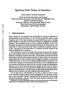
Besides gauge invariance, one of the main features of the model is its general covariance. Indeed, the physics of the system (2.1) is independent of the particular choice of the metric that one can introduce in the three-dimensional space. General covariant quantum field theories are not a novelty in physics; one of the reasons which makes the model (2.1) somewhat special is the fact that general covariance is achieved not by integrating over the space of metrics. The action (2.1) is independent of the metric and, as long as one is interested in the expectation values (2.5), the introduction of a metric is not required. These features of the model suggest that ( W ( L ) ) is related to some invariants characterising the link L. In order to discuss this relationship we recall some basic notions from knot theory [4,11]. Consider two links L 1 and L 2. They are called ambient isotopic (L 1 - L2) if there exists a smooth deformation through embeddings from one to the other. A practical procedure for verifying ambient isotopy is the following one. We associate with any link L a four-valent planar diagram, namely a diagram obtained by projecting L on a plane in such a way that the projection contains only simple crossing points where the choice of o v e r / u n d e r crossing is given. It can be shown that L~ - L 2 if and only if there is a finite sequence of Reidemeister moves, shown in fig. 1, which changes the diagram of L 1 into the diagram of L 2. It is useful to introduce also the concept of regular isotopy for diagrams [4]. Two diagrams are said to be regular isotopic if one can be obtained from the other by a sequence of Reidemeister moves of type II and type III only. Regular isotopy arises for example when, instead of a link, we consider an oriented twisted band. Clearly, the Reidemeister moves of type I do not relate ambient isotopic bands, see fig. 2. It turns out that the ambient isotopy of twisted bands is equivalent to regular isotopy for link (or knot) diagrams. Now we introduce the H O M F L Y polynomials [5,6,12]. To each oriented link there is associated a finite Laurent polynomial PL(t, Z) of tWO variables with integer

P. Cotta-Ramusino et al. / Link invariants

561

I

III)

Fig. 1. Reidemeister moves of type I, II and III.

coefficients, such that if L 1 - L 2 , then PL1 = PL2" The polynomial P L c a n be constructed by means of the skein relation

tPL+- t-IPL = ZPLo.

(2.8)

Here, the diagrams associated with L + , L and L 0 differ only at the site of one crossing as shown in fig. 3. By means of eq. (2.8) and Reidemeister moves of all the three types, the polynomial of any link can be reduced to a sum of polynomials for unknotted links. In this way one can construct recursively PL for any L starting from the polynomial P0 of the unknotted knot which is usually normalized to the unity, P0 = 1. It is known [4, 6] that the relation (2.8) determines uniquely the link invariant PL- Unfortunately, it is also known that PL does not determine uniquely the link L up to ambient isotopy. The link invariant PL(t = 1, z) is known as the

Fig. 2. A twisted band is not invariant under Reidemeister moves of type I.

562

P. Cotta-Ramusino et al. / Link invariants

L+

L.

Lo

Fig. 3. Configurations related by the skein identity.

Alexander-Conway polynomial [13], whereas PL(t, Z----V~-- 1 / ~ - ) is the Jones polynomial [3]. For discussing the properties of Wilson line operators (W(L)), it is necessary to consider the so-called R-polynomial introduced by Kauffman [4,14]. Differently from PL, R L is not ambient isotopy invariant but only regular isotopy invariant. R L is defined by the exchange identity RL+-- R L =ZRLo,

(2.9)

supplemented by RL+= aRL0,

(2.10), (2.11)

RL = a-IRLo,

where L + , L and 6 0 are displayed in fig. 4. In analogy with the PL-polynomials, R L ( a , z) can be constructed recursively (R 0 = 1); however, differently from the PL polynomials, in the case a ¢ 1 one is not allowed to use Reidemeister moves of type I, but instead is bound to use eqs. (2.10) and (2.11). Now, the important point to note is that RL(a, z) can also be interpretated as an ambient isotopy invariant for oriented twisted bands [9], where a is the variable which measures the twisting in the band. As shown by Kauffman, PL and R L are closely related. In fact one has (2.12)

PL ( t = a, Z) = a-w(L)RL ( a, Z ) ,

where the writhe w(L) is given by w(L) = E c ( p ) .

(2.13)

p

The sum in (2.13) is performed over all crossings of the diagram associated with L

-©"L÷

.©. i._

-i.o

Fig. 4. Configuration related by eqs. (2.10) and (2,11).

P. Cotta-Ramusino et al. / Link inoariants

563

and {(L+) = +1.

(2.14)

One should note that the writhe w(L) is regular isotopy invariant, it is additive and can be computed by analyzing locally the diagram associated with L. Eq. (2.12) will be proven, in a more general context, later on. Summarizing, one can associate a polynomial to every planar diagram; how to construct this polynomial is specified by a set of local rules. The key ingredients are: (i) the behaviour under Reidemeister moves; (ii) the skein relation. So far, we have discussed two different possibilities. In the first, one associates with a link L the PL-polynomial. In this case it is assumed that PL is invariant under all the Reidemesiter moves and the skein relation (or exchange identity) is given by eq. (2.8). In the second possibility, the RE-polynomial is not invariant under Reidemeister moves of type I, but it is rather "covariant", see eqs. (2.10) and (2.11). In addition, one has the exchange identity (2.9). Comparing eqs. (2.8) and (2.9), we see that the latter can be generalized by introducing a new variable fl, which is the analogue of t. We define then the regular isotopy invariant polynomial SL(a, fl, z) by means of the "generalized" skein relations

&+= SLo,

(2.15)

S L = a 1SL0,

(2.16)

(2.17)

/ ~ S L . ~ - - / ~ - 1 S L = ggLo ,

supplemented by the standard normalization condition So = 1

(2.18)

for the unknot. As we shall see later, in this form the skein relations are directly applicable to (W(L)). Similarly to the Re-polynomial, S e also can be related to PL- One proceeds as follows. Since both SL and w(L) are regular isotopy invariants, the same holds for the " n e w " polynomial

NL(a, fl, z) -- a-w(L)Se(a , fl, z). Let us find the generalized skein relations satisfied by immediately that NO= 1.

N L.

(2.19) From (2.18) it follows (2.20)

564

P. Cotta-Ramusino et aL / Link invariants

Consider now NL+. From eqs. (2.13) and (2.14) one finds

w(t+)= 1 + w(to).

(2.21)

Therefore, using eq. (2.15) one gets NL+=

a

w(L+)sL+= a

w(Lo)Sgo= NLo-

(2.22)

Analogously, N L = NLo.

(2.23)

Eqs. (2.22) and (2.23) show that N e is actually ambient isotopy invariant. Finally, consider the exchange identity, (a/3)NL+-- (or/3)-1N L = (Ot/3)ot-w(L+)SL+-- (Or/3)-la-w(L-)SL_ = a-w(L°)(flSL+-- fl-aSL_ ) = za-w(L°)SLo = ZNLo.

(2.24)

Eqs. (2.20) and (2.22-2.24) imply, in view of (2.19), that

PL ( t = aft, z) = a-w(L)SL ( a, /3, Z ).

(2.25)

Since the Re-polynomial is a particular case of the Se-polynomial (with/3 = 1), the above argument proves also eq. (2.12). Some final comments are in order. On the level of ambient isotopy for links (PL-polynomial) there is no need for introducing separately a and /3. However, as far as {W(L)) is concerned, the ambient isotopy of bands (framed links) is relevant. This is the reason why we have introduced the SL-polynomial and why the distinction between a and /3 is physically meaningful. If one interprets {W(L)) as the quantum mechanical amplitude of a charged particle with fractional statistics moving along L, then a can be understood as the phase change of the wave function under a 2rr spin rotation. 3. Variational derivation of the skein relation

In this section, we concentrate on the expectation value (W(L)). Our strategy in deriving the associated skein relation is to study the behaviour of (W(L)) under infinitesimal deformations of the contour defining L*. A first question one may ask is whether ~W(L)) is ambient isotopic; in other words, is (W(L)) invariant under continuous deformations of L? In what follows we will first answer this question. * We thank very much L.H. Kauffman who, while referring to some work in progress by L. Smolin, suggested to us that a variational approach to the skein invariancecould be considered.

P. Cotta-Ramusinoet al. / Link invariants

565 2

(a)

1~

(~) Fig. 5. An F~.-insertion at the point x on the Wilson line.

Let us focus on the part

U(xl, x2)=Pexp,f •

X2

p,

a

a

dx A,R

(3.1)

X1

of the Wilson line operator associated to the oriented path along L connecting two arbitrary points x I and x 2 (see fig. 5a). As is well known, an infinitesimal variation of the path in x produces the F~,-insertion (see fig. 5b) U ( x l , x2) ~ U ( x l , x ) i Z ~ F ~ ( x ) R " U ( x ,

(3.2)

x2).

Here there is no summation over/~ and v, S "" = d x # d x ~ is the area element and a=

A~

~

(3.3)

fah';4bA ".

In order to evaluate the effect of the F~,-insertion on (W(L)), we make use of the following remarkable property of the Chern-Simons theory: ( FA; ( x ) 0102 . . . ) -- Z - I f ~ A e'r Ffl, ( X ) Ol02 . . .

(4°)

e/r

= z - ' f ~ A -i T '.~OSA;(x)

O102"'"

~A-(~(O102...).

(3.4)

In deriving the relation (3.4), eq. (1.1) has been used and an integration by parts has been performed. Combining eqs. (3.2) and (3.4) one gets

( . . . U ( X l , X2)... 47r -i--83(x-y)%~oX""dy°(. k

U(Xl, x)Y'~R~R~U(y, .

.

6l

.

.

x2)..

)

(3.5)

566

P. Cotta-Ramusino et al. / Link invariants

The differential d y p in the factor v -- 63(x - y ) % . o N " " d y ° ,

is oriented along the tangent to the path. Being the product of a volume element with a 63-function, v is dimensionless and can take the values 0 or +1. If d y p belongs to the plane determined by E"", then v = 0. Otherwise v = +_1, depending on the orientation of Z "" with respect to d y °. (Clearly the orientation of the ambient space is fixed by the choice of %,p.) Therefore, under infinitesimal deformations of L, one has three possibilities 6 ( W ( L ) ) = 0,

(3.6)

or 4~

6(W(L)) = -T-i~-c2(R)(W(L)),

(3.7)

where c2(R ) is the quadratic Casimir operator in the representation R, c2(V.)l = E RaR o"

(3.8)

a

How should one interpret eqs. (3.6) and (3.7)? First of all eq. (3.7) shows that (W(L)) is not ambient isotopic. Therefore (W(L)) cannot be directly associated with a PL-polynomial. One can hope, however, to relate (W(L)) to a SL-polynomial. In fact, we will show that (W(L)) satisfies the generalized skein relations (2.15)-(2.17). In order to do this, we would like to translate eqs. (3.6) and (3.7) in terms of diagrammatic relations. There are essentially three ways of assigning diagrammatically a small area to a local deformation of L. The first one is to use the diagram Lf (displayed in fig. 6) in which d y ° belongs to the plane determined by ~"", whereas the remaining possibilities are related with the diagrams [ + and L shown in fig. 4.

A

/f X

Fig. 6. Planar deformation in which the tangent to the path in x belongs to the plane of the deformation.

567

P. Cotta-Ramusino et al. / Link invariants

We propose the following diagrammatic interpretation of eqs. (3.6) and (3.7). This interpretation will be subjected later to several checks. Eq. (3.6) means (wG))

=

(3.9)

whereas eq. (3.7) is equivalent to 4q7

(W(L+)) - (W(L )) = -i~-c2(R)(W(Lo) )

(3.10)

in the small area limit of the locks in L+ and 6 . Clearly the other choice for the sign on the r.h.s, of eq. (3.10) is equivalent to the exchange L + ~ L . To make contact with the SL-polynomials, eq. (3.10) can be rewritten as

(W(L+))=a(W(Lo)),

(W(L_))=a-I(W(Lo)),

(3.11), (3.12)

where

a=l-i-ff-c2(R )+O

(1)

-

(3.13)

Comparing eqs. (3.11) and (3.12) with eqs. (2.15) and (2.16) we interpret a as the variable measuring the twisting of the band, that is, the framed link. In eqs. (3.11) and (3.12), the small area limit picks up the first two terms in the expression (3.13). Because of eq. (1.1), any subsequent variation of the path contributes a factor 2w/k and by taking into account also the higher dimension operators involved in a finite deformation of the path, in principle one could determine the O(1/kZ)-part of a. We shall not elaborate on this point here. Note that for the action (2.1), 2~r/k plays the role of h; this allows for a perturbative check of eq. (3.13). Later on, we will verify to the first non-trivial order in 1/k that the value of a given by eq. (3.13) coincides precisely with the variation of (W(L)) under a change of framing in the perturbative approach. We proceed now by looking for an exchange identity for (W(L)) which plays the role of eq. (2.17). A way of relating L+ and L , displayed in fig. 3, is shown in fig. 7. For the infinitesimal area of the circle in fig. 7 one can apply once more the variational method used before. One has (W(L+) 5=(W(L

)5 + ( - . - U ( 1 , x ) i Z u " F f l ~ ( x ) R ~ U ( x , 2 ) - - - U ( 3 , 4 ) - - . ) -

(3.14)

At this stage F~(x) can be replaced by a functional derivative with respect to A~(x), which acts on both the paths 1---, 2 and 3 ~ 4. Since by definition the crossing should not involve any twisting, the functional derivative in A~ must act trivially on U(1,2). This means that d y p for the path 1 -~ 2 belongs to the plane

568

P. Cotta-Rarnusino et al. / Link invariants 1

4

3

1

2

>d 4

3

2

Fig. 7. How to relate overcrossing with undercrossing.

determined by Z ~". In other words, for the path I --) 2 one should apply eq. (3.6) (or eq. (3.9)). So, one finds 4¢/

(W(L~))=(W(L))-i-~-~(...U(1,x)R"U(x,2),..V(3,

x)R'"U(x,4)...).

a

(3.15) Note that the paths 1 ~ 2 and 3 ~ 4 do not belong necessarily to the same component of L; in general the representations of G assigned to 1 ~ 2 and 3 ~ 4 are different and have been denoted in eq. (3.15) by R and R' respectively. At this point we would like to relate the second term on the r.h.s, of eq. (3.15) with (W(L0)). The simplest case in which this can be achieved is when a Fierz identity for the sum ,.~,v"R"ijR'"kl exists. Taking G = S U ( N ) and R" -- R '~ = T a one has 1

~_, T~T{~ = ½8,,3jk - ~--~3ij3k,

(3.16)

a

and in this case eq. (3.15) takes the form 27r 1 \ ( W ( L + ) ) = 1 + i--£----~)(W(L_))

Since ( W ( L + ) ) differs from ( W ( L ) )

27r

-iT(W(L0)).

(3.17)

by O ( 1 / k ) , eq. (3.17) can be rewritten as

]3(W(L+)) - ]3-~(W(L )) --- z ~ W ( L o ) ) ,

(3.18)

where fl=l-i

k 2N + O

,

(3.19)

and z = -i~-- + 0

(3.20)

569

P. Cotta-Ramusino et a L / Link invariants

13

-

!e,

=

z

Fig. 8. Diagrammatic representation of eq. (3.21).

As before, the O(1/k 2) terms in eqs. (3.19) and (3.20) take into account higher order corrections. Eqs. (3.11), (3.12) and (3.18) show that the expectation value (W(L)) of the Wilson line operator in the fundamental representation of SU(N) obeys the generalized skein relations (2.15)-(2.17) of a SL-polynomial. This is one of the main results of our investigation. A first consistency check of eqs. (3.11), (3.12) and (3.18) is the following. For the Wilson line operators in the fundamental representation of SU(N), eq. (3.18) implies (see fig. 8)

B