Quantum Field-Theory Models on Fractal Spacetime - Project Euclid

Communications in Commun. Math. Phys. 125, 613-636 (1989)

Mathematical

Physics

© Springer-Verlag 1989

Quantum Field-Theory Models on Fractal Spacetime I. Introduction and Overview

G. Eyink* Department of Physics, The Ohio State University, Columbus, Ohio, USA

Abstract. The present work explores the possibility of giving a nonperturbative definition of the quantum field-theory models in non-integer dimensions, which have been previously studied by Wilson and others using analytic continuation of dimension in perturbation integrals. The method employed here is to base the models on fractal point-sets of non-integer Hausdorff-Besicovitch dimension. Two types of scalar-field models are considered: the one has its propagator (= covariance operator kernel) given by a proper-time or heat-kernel representation and the other has a hierarchical propagator. The fractal lattice version of the proper-time propagator is shown to be reflection-positive. The hierarchical models are introduced and their properties discussed on an informal basis.

1. Introduction

In a classic 1973 paper, "Quantum Field-Theory Models in Less Than 4 Dimensions," Wilson studied the scalar interaction φA and Fermi-type (Gψψ)2 interaction for spacetime dimension between 2 and 4 [45]. His method was perturbative (although in some cases infinite classes of diagrams were summed within a ί/N expansion) and the integrals associated to the Feynman-graphs were extended to noninteger d by the analytical continuation procedure introduced earlier as a regularization method for gauge theories [10, 33]. Since that time the question of what non-perturbative significance might be given to these models - if any - has remained open. However, more recently Gefen, Aharony, Mandelbrot and collaborators have made a relevant investigation of the possibility of achieving statistical-mechanical spin models, with the critical properties predicted by the ε-expansion method, by employing fractal lattices [25-30]. In this paper the same method is exploited to give a non-perturbative definition of quantum field* Presently at Rutgers University, New Brunswick, NJ. This paper is based largely on the thesis presented by the author for the degree doctor of philosophy in physics at the Ohio State University in 1987

614

G. Eyink

theory models in non-integer dimensions. These models are interesting as theoretical toys to illuminate the possibilities of quantum field-theory, as argued by Wilson in the conclusion of his paper: "... it seems likely that a thorough study of these models in less than four dimensions will generate new ideas about the nature of field theory that do not depend on dimensionality and may apply to four-dimensional theories as well. It should be instructive to study the behavior of high-energy scattering, deepinelastic scattering, bound states, etc. in these models." Wilson himself discovered a number of interesting phenomena in these models. For example, he exhibited the possibility of anomalous scaling at high energies due to a non-Gaussian ultraviolet renormalization-group fixed point. Also, he argued for the equivalence - in dimension d just less than 4 - of four-fermion (ψψ)2 theories and Yukawa theories when these are defined by unconventional renormalizations. It is indeed possible that these models in 4 —ε dimensions are actually physically relevant. In [14] Crane and Smolin motivate the consideration of fractal spacetimes, or "fractal spacetime foam," by quantum gravity considerations. Elsewhere the relevance of such models to problems of particle physics, particularly the Higgs sector of GUT's models, is considered [17]. However, in the present paper and its companion [19] we shall simply introduce and study two scalar-field "Euclidean" theories on fractal point-sets. We hope by this investigation to have demonstrated that fractal sets provide an effective and feasible method of realizing quantum field-theory in non-integer dimensions, at least for the scalar theories. The case of higher-spin fields, e.g. gauge fields and fermions, pose a vastly more difficult problem. Although some progress can be made on this problem by purely formal considerations [18], at this time there is really no rigorous framework for introducing spin structure into fractal sets. It is not clear therefore whether the fractal continuation applies to all the physical theories for which the usual analytical continuation is effective. The plan of this paper is as follows: in the following Sect. 2 the fractal sets employed in this work - which are amenable to a rigorous mathematical treatment - are introduced and discussed. In Sect. 3, scalar field theory models on fractal sets with propagator given by a proper-time or heat-kernel representation are defined. It is shown that this approach leads to actual quantum-mechanical models with positive-norm Hubert space. The scaling and renormalizability properties of these models are then discussed. In the final Sect. 4, hierarchical-type scalar field-theory models on fractal sets are introduced, for which the renormalization problem can be solved in a rigorous fashion, employing the large-field and analyticity techniques of Gawedzki and Kupiainen [22-24]. We content ourselves here with an informal discussion of the model and its analysis. Precise statements of results and complete, rigorous proofs for the hierarchical model approximation are contained in the companion paper [19].

2. Fractal Spacetimes

The purpose of this section is to introduce and briefly discuss the fractal point-sets employed in this paper and also to set the notations.

Quantum Field-Theory Models on Fractal Spacetime. I

B

615

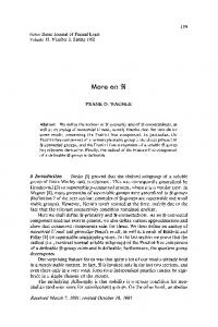
Fig. 1. Three stages in the construction of a Sierpinski carpet ΊF°(d,L,^\ with d = 2, L = 3 and ^ = {(1,1)}. The set has fractal dimension J=log8/log3. The origin is labelled as 0

The most important class of fractal sets for our purposes are the Sierpinski carpets [42], which are two-dimensional generalizations of the well-known Cantor middle-thirds set. As a simple case, consider the set obtained from the unit square [0,1] 2 by partition into 9 subsquares and removal of the central open subsquare, repetition of the same operation on the 8 remaining closed subsquares, etc. Generalization is possible both with respect to the Euclidean dimension d, the (integral) scale factor L, the edge-length LN of the initial hypercubes, and the set Ή of sub-hypercubes removed at each stage. The various sub-hypercubes are labelled by d-component vectors with components ranging from 0 to L— 1. We denote the corresponding fractal set by ¥N(d, L, #). It has Hausdorff dimension = log(Ld-C)/logL,

(2.1)

where C = \, and Pd(x, y) the heat-diffusion kernel and PdN(n,m) = (jι\ TN |m> the matrix of JV-step transition probabilities. There is no difficulty to introduce fractal lattice analogues of the proper-time representations and we shall do this first, establishing certain relevant properties, such as the reflection-positivity. To introduce propagators on fractal continua by means of a proper-time representation requires the proper mathematical definition of "Brownian-motion processes" on these objects, a problem now much investigated [5, 6, 32, 34]. We have fewer hard results in this case, but we shall discuss it briefly with a view of explaining the significance for quantum fieldtheories of known and conjectured results. If T is a transition probability matrix on any of the unit-spacing fractal lattices 2 2 F£ earlier introduced, then the bounded operator T:/ (F£)->/ (F£) defined by

(Tf)(n)= ΣJ«mf(m)>

(3-7)

fεlΨl)

meFo

is easily seen to be a contraction. If one further requires that T be symmetric, Tnm=Tmn,

m,ne¥d0,

(3.8)

then T is self-adjoint, so that, if (3.1b) is made a definition, (3.9)

-A=2d{l-T), 2

d

it follows that the operator — A is positive, self-adjoint on l {W 0). Therefore the definition is a reasonable one. Also, if T is a nearest-neighbor RW, \n-m\>ί=>Tnm

= 0,

(3.10)

622

G. Eyink

then — A has the same property, i.e. it is local. The set of symmetric, nearestneighbor RWs on the fractal lattices introduced above, F0(d) and Q ;

(3 4 ? )

2a

or, likewise, existence of the limit M

d

M

M

P?(X,JO= lim L ~ Pίd.L2M/θτ{lL xllL y}),

(3.48)

M->oo

for τ > 0. In these formulas, [x] is the element of FQ nearest to x EFQ according to some conventional assignment. Obviously, these limits, if they exist and are nontrivial for some 3, θ, imply (3.42), (3.43). In the case of the Sierpinski gasket we can carry out a version of this scaling limit and establish the scaling law (3.42). This relation as well as the existence of the heat-diffusion process and many fine sample-path properties have already been established in [5]. However, since the Sierpinski carpet case appears more difficult, it may be useful to record an alternative approach. The present proof is based upon an exact renormalization-group equation for the lattice Green's function, G0(n,ra; z), due to Rammal [39]. We simply quote here the result (for d = 2): G0(n,m; z') = Γ W 0 (2n,2m; z)

(3.49)

z' = z2/(4-3z)

(3.50)

Γ 1 W = z(2 + z)/(4 + z)(2-z).

(3.51)

with

and The RG transformation (3.50) has two fixed points on the unit interval [0,1], a stable fixed point z* = 1 and an unstable fixed point z* = 0. For z = 1 — ε, 0 < ε ]; z) with

(3.54)

Z τ + i U\q\s, •)/ + - ,

y'(s) = L\q(s, •)> - ^ L2\q2(s,

where the expectations are with respect to dμ(z) = e~z2/2dz/(2π)1/2. initial spin weight exponent w in the form

(4.11)

We take our

^«:s4:Go + ^ ί ^ 6 : G o

w(s)= j}r:s2:Go+

(4.12)

Here, :F(s):Go denotes the normal-ordering with respect to covariance G o :

'Fίs] : G o ^exp Γ - \

G0(n,m)d2/dsndSn]F[5] .

£

(4.13)

We drop the subscript G o as convenient. In this form, it is easy to see that the RG transformations diagonalizes to firstorder: . 1 1 ^L2:s2:

L\q}=

+ ^L-2(1"£)i:56:.

+ -Πw.s*:

(4.14)

The second-order contribution is also easily calculated from (3.9-12) and yields f

2

f

y(s) = y\O)+^r :s : w i t h

/

4

f

+ ~u :s :

2

6

+ ^t :s :+...

2

2

r = L [r-(α 2 w + α1rM + α 3 r + K 2 )], 2

u! = Π[u-{β2u

+ β1ru+U2)]9

2

2

> = L~ ^-\t-{δ2u

+ T2)'\.

t

(4.15) (4.16) (4.17)

(4.18)

The ... in (4.15) represents higher-order induced terms, like — h ' : s 8 : , which, 8! however, on assumptions on the initial weight (4.12), will be seen to be negligible. R2, U2, T2 are homogeneous, second-order multinomials in r, u, t representing quadratic contributions other than those distinguished. The coefficients α l 5 α 2 , α 3 , βu βi> 2, etc. are all 00) as L / + oo and, in particular, oc1 >0, β2>0. Let us assume initially that u = O(εL-~d\ogL), a

r = O(εL" logL), 2

a

ί = O(ε L~ logL).

(4.19) (4.20) (4.21)

G. Eyink

632

It is clear from (4.17), (4.18) that (4.19), (4.21) are preserved under iteration. Also, we 3 d 3 note that higher power couplings, like h\ are O(ε L~ log L) at least. Because of the relevancy of the variable r, we cannot automatically conclude that d Ϋ = O(εLΓ log L). However, this is true for r located initially on the critical hypersurface, r = rc(u, t). The critical surface must pass through (r, u, t) = (0,0,0) 2 and, since t = 0(βu ), we conclude that rc(u, t) = O(u). By this observation the RG 2d 3 equations for r, u decouple from those of the other variables to O(L u ): in 2d 3 particular, terms like α 4 rί = O(L u ) may be neglected. If we parameterize the critical hypersurface by:

φ) = rίcu + r2cu2

(4.22)

and use the stability condition (4.23) with (4.22) and (4.16-17), we find that (4.24)

and (4.25)

or Only a single interaction equation is now of concern: i3)].

(4.26)

The fixed points of (4.26), (4.22) in the chosen domain (4.19-21) are then seen to be (r, u) = (0,0) = 0 and (r*, u*) = F with w

* = β- i(l _ L~ε) + O(ε 2 L" a log 2 L) = O(εL~~d logL), 2

3

a

3

2

a

r* = r2c(w*) + O(ε L- log L) = O(ε L" logL).

(4.27) (4.28)

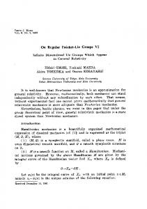
The linearized RG flow diagram for the model in the small-coupling domain is sketched in Fig. 9.

Fig. 9. The RGflowof the hierarchical model for r, u = O(εL d logL). The Gaussian fixed point, 0, the W—F fixed point, F, and the critical hypersurface, OFC, are indicated

Quantum Field-Theory Models on Fractal Spacetime. I

633

Now, as usual, if we consider the "Euclidean" hierarchical scalar field-theory on Fjϋ with path measure

J

L-M~dv(Φ(n))]dμGM(φ)

Σ

-

xexpΓ-

L-MMφ(n))\dμGM{φ),

Σ

(4.29)

where 00

GM(n,

m)=

L

Σ k=

~

akδ

-M

iL - (fc + i)π]f t L - (fc + ^ΊA{nk)A{mk),

(4.30)

one can relate the Green functions of (4.29) with the statistical correlation functions of (4.1) by a simple rescaling φ(n) = LM«i2sLMn,

(4.31)

w(s) = L~Mdv(LMθί/2s).

(4.32)

with the definition One finds (4.33) Clearly, the renormalization problem, to find a sequence of cutoff dependent interactions υ(M) so that the limit of the left-hand side of (4.33) exists as M /* + oo, is equivalent to the problem of finding a sequence of spin-weights w(M), so that the scaling limit, M / + oo, of the right-hand side exists. It is also useful to reformulate the renormalization problem in terms of the Green's functions (« 1? ..., np; v{M\ N) of block-averaged fields

L

kl

L^M~k)d meD[ M '(n)

Σ

Φ(m),

(4.34)

m:lLkmJ = n

defined as GiM\n1,...,np;υ