Quantum Fields as Operator Valued Distributions and Causality

Quantum Fields as Operator Valued Distributions and Causality ´ Pierre GRANGE Laboratoire de Physique Théorique et Astroparticules Université Montpellier II, CNRS, IN2P3 CC 070 - Bat.13 - Place E. Bataillon F-34095, Montpellier, Cedex 05 - FRANCE

Ernst WERNER

arXiv:math-ph/0612011v2 8 Feb 2007

Institut f¨ ur Theoretische Physik D-93040, Universit¨ at Regensburg - GERMANY (Dated: February 6, 2008) Quantum Field Theory with fields as Operator Valued Distributions with adequate test functions, -the basis of Epstein-Glaser approach known now as Causal Perturbation Theory-, is recalled. Its recent revival is due to new developments in understanding its renormalization structure, which was a major and somehow fatal disease to its widespread use in the seventies. In keeping with the usual way of definition of integrals of differential forms, fields are defined through integrals over the whole manifold, which are given an atlas-independent meaning with the help of the partition of unity. Using such partition of unity test functions turns out to be the key to the fulfilment of the Poincaré commutator algebra as well as to provide a direct Lorentz invariant scheme to the Epstein-Glaser extension procedure of singular distributions. These test functions also simplify the analysis of QFT behaviour both in the UV and IR domains, leaving only a finite renormalization at a point related to the arbitrary scale present in the test functions. Some well known UV and IR cases are examplified. Finally the possible implementation of Epstein-Glaser approach in light-front field theory is discussed, focussing on the intrinsic non-pertubative character of the initial light-cone interaction Hamiltonian and on the expected benefits of a divergence-free procedure with only finite RG-analysis on physical observables in the end. PACS numbers: 11.10.Ef, 11.10.St, 11.30.Rd

I.

INTRODUCTION

Causal perturbation theory (CPT) goes back to ideas from Stueckelberg, Rivier and Green [1], Bogoliubov, Parasiuk and Sirkov [2] and has been developed by Epstein and Glaser [3] and more recently by Scharf [4]. A little after Epstein and Glaser came formulations [5] to construct finite gauge theories, based on regulator free momentum substraction schemes. In the last publication the questions of the finiteness of Lorentzinvariant amplitudes and of symmetry conservation are treated seperately. Moreover, as opposed to CPT, the importance of causality issues in relation to the finiteness problem itself is not of main concern. In CPT the S-matrix is constructed as a formal functional expansion in an unimodular interaction-switching test function. Whereas in the traditional approach the S-matrix amplitudes are determined by equations of motion, in CPT they are determined inductively by causality conditions imposed on switching test functions. Such causality conditions turn out to be as stringent for the S-matrix evolution as the equations of motion themselves. On an heuristic level it may be seen as follows: if g1 (t) and g2 (t) are two such switching test functions with supports such that supp[g1 ] ∈ (−∞, s) and supp[g2 ] ∈ (s, +∞) respectively, then causality implies that S(g1 + g2 ) = S(g1 ) · S(g2 ), which is the functional equation for an exponential.

The S-matrix amplitudes are time ordered products of operator valued distributions (OPVD). They are split into causal advanced and retarded pieces, in such a way that any singular behaviour at equal space-time points is avoided. The procedure has long been recognized as mathematically rigorous [6, 7] since it is divergence free at each iteration stage. Nevertheless Epstein-Glaser work almost fell into oblivion among QFT practioners mainly because (1) in its original version there were difficulties in disentangling the multiplicative structure of renormalization and (2) the rise of renormalization group methods turned research interests into this direction. However Epstein-Glaser approach still enjoys popularity in the world of mathematical physicists dedicated to the construction of a rigorous and mathematically well defined QFT [8–10]. In this context the key issue is the extension of singular distributions to the whole spacetime manifold. In mathematics a rigorous way to define an extension of a singular distribution is a weighted Taylor series surgery: one throws away an appropriate jet of the test function at the singularity and defines the extended distribution by transposition at the level of the functional from the corresponding Taylor remainder of the test function. Transposed to Fourier space the procedure amounts to a substraction method [10] which in-

2 cludes BPHZ renormalization [2, 11] as a special case. In a Minkowskian metric this is equivalent to the implementation of causality while in its Euclidean counterpart it is a symmetry preserving prescription for substractions. In light-front quantum field theory (LFQFT) there is a compelling reason to introduce test functions related to the consistency of the canonical quantization scheme itself. It is best seen for the massive scalar field. The form of the LF-Laplace operator leads to a hyperbolic equation of motion which requires initial data on two characteristics. Canonical quantization in terms of initial field values in the light cone time is however possible + ) + provided [12] limp+ →0 χ(p p+ = 0,where χ(p ) is the field amplitude at p+ = p0 + p3 . With fields as OPVD this + ) relation becomes limp+ →0 f (p p+ , which is surely satisfied for the class of test functions f (p+ ) used for the Fock expansion of the field operators [13, 14]. Our earlier approach with test functions [13, 16] in fact implements Epstein-Glaser treatment of singular distributions in the LFQFT context. Here we want to assess our particular choice of test functions as ‘partition of unity‘ and show the resulting simplifications brought about for the treatment of Poincaré’s invariance and for the Lorentz invariant Taylor series surgeries discussed in [10]. In Section II the general definition of fields as OPVD is given. Due to specific properties of Euclidean manifolds it is shown that the class of admissible test functions can be restricted to a ‘partition of unity‘, in close analogy with the usual atlas-independent definition of integrals of differential forms. Thus a QFT construction is possible, which is test-function independent. As a consequence, for scalar field theory it is shown that Poincaré’s commutator algebra is fulfilled, in contrast with the case of arbitrary test-functions. In Section III the BogoliubovEpstein-Glaser expansion of the S-matrix is recalled. It is given in terms of the interaction-switching test function g ∈ D′ (IR 4 ). The proper Epstein-Glaser time ordered construction of the expansion coefficients is described. The implementation of Lorentz covariance of the procedure is presented and the simplifications brought about with test functions vanishing at the origin with all their derivatives are shown. They concern Lorentz covariance, the Taylor surgery itself and its interpretation in terms of the BPHZ renormalisation scheme. In Section IV, the use of Lagrange’s formula [8, 10] for Taylor’s remainder in connection with partition of unity test functions is shown to simplify also the analysis of singular distributions both in the IR and UV domains. A direct application of the method in the IR is shown to be successful for the free massive scalar field theory developed in the (conventionally hopeless) mass perturbation expansion. It should also prove relevant to many problems of massless conformal field theories (CFT). Finally, following [17], in the UV the alternative interpretation of the effects of partition of unity test functions in terms of Pauli-Villars type subtractions at the level of propagators is pointed out

in Euclidean and Minskowskian metrics. In Section V Epstein-Glaser separation method of Section III for distributions into advanced and retarded pieces (splitting procedure) is rephrased for the special case of partition of unity test functions. Their use simplifies greatly the derivation of the relation between the splitting procedure and dispersion relations. In Section VI a general discussion is given on the possibility of applying BSEG’s method in a non-perturbative Light Front Quantization framework and on the benefits one might expect from the procedure. Finally some conclusions are drawn in Section VII.

II. FIELDS AS OPVD, PARTITION OF UNITY ´ COMMUTATOR ALGEBRA AND POINCARE A.

Fields as OPVD

The history of fields as OPVD is almost as old as Quantum Field Theory itself. In fact the mathematical developments of Distribution Theory (or Generalized Functions) [18, 20] in the 1960′s were intimately related to problems raised at that time by pioneers in the QFT formulation. This mutual feedback has lead to QFT formulations [21] in the 1960 − 70′s which aimed at dealing in a mathematically consistent way with intrinsic divergences crippling the usual QFT perturbative analysis. Among these approaches the work of Epstein and Glaser [3] has long been recognized as mathematically rigourous and free of undefined quantities. It is still generating an important literature in mathematical physics and we shall summerise here some of its recent developments. To introduce fields as OPVD one may consider, without loss of generality, the free massive scalar field in Ddimensions. The general solution of the Klein-Gordon equation is a distribution, ie an OPVD, which defines a functional with respect to a test function ρ(x) belonging to D(IR D ), the space of Schwartz test functions [18], Φ(ρ) ≡< φ, ρ >=

Z

d(D) yφ(y)ρ(y).

(II.1)

Here Φ(ρ) is an operator-valued functional with the possible interpretation of a more general functional Φ(x, ρ) evaluated at x = 0. Indeed the translated functional is a well defined object [18] such that Tx Φ(ρ) = < Tx φ, ρ >=< φ, T−x ρ > Z = d(D) yφ(y)ρ(x − y).

(II.2) (II.3)

Now the test function ρ(x − y) has a well defined Fourier decomposition ρ(x − y) =

Z

d(D) q expiq(x−y) f (q02 , q 2 ). (2π)D

(II.4)

3 It follows that Z (D) d p −ipx 2 e δ(p − m2 )χ(p)f (p20 , p2 ). Tx Φ(ρ) = (2π)D Due to the properties of ρ, Tx Φ(ρ) obeys the KG-equation and is taken as the physical field ϕ(x). After integration over p0 and with ωp2 = p2 + m2 the quantized form is taken as the (D − 1)−Euclidean integral ϕ(x) =

Z

d(D−1) p f (ωp2 , p2 ) + ipx [ap e + ap e−ipx ]. (II.5) (2π)(D−1) 2ωp

f (ωp2 , p2 )

acts as a regulator [13, 14] with very specific properties [15]. This expression for ϕ(x) is particularly useful to define correlation functions of the field and more precisely in the light-cone (LC) formalism because the Haag series can be used [16] and is well defined in terms of the product of ϕ(xi ). In the full Euclidean metric there is no on-shell condition and ϕ(x) stays a D-dimensional Fourier transform with f (p2 ) only. It might appear that there would be as many QFT’s as eligible test functions. However some importants results from topological spaces analysis may be invoked. Some general definitions need first to be recalled : Definitions: a) An open covering of a topological space M is a family of open sets (Ui )i∈I such that M = ∪i∈I Ui . b) An open covering (Ui )i∈I is said to be locally finite if each point of M has a neighbourhood which intersects only a finite number of the (Ui ). c) A topological space M is paracompact iff every open covering (Ui )i∈I admits a locally finite refinement (that is a locally finite open covering (Vj )j∈J with the property that for all j ∈ J there exists i ∈ I such that Vj ⊆ Ui ). d) If (Ui )i∈I is an open covering of M, a partition of unity subordinate to (Ui )i∈I is a family (βj )j∈J of positive continuous functions on M such that (i) For all X ∈ M there exists a neighbourhood UX of X such that all but a finite number of the βj vanish on UX . (ii)

P

i∈I

βi (X) = 1 for all X ∈ M.

(iii) For all j ∈ J, there exists i ∈ I such that the closure of {X ∈ M : βj (X) 6= 0} is contained in Ui . The closure of {X ∈ M : βj (X) 6= 0} is called the support of βj . Remark: If (αi )i∈I and (βj )j∈J are two partitions of unity subordinate to (Ui )i∈I and (Vj )j∈J respectively, (αi βj )(i,j)∈I×J is a partition of unity subordinate to

(Ui ∩ Vj )(i,j)∈I×J . Since this property is crucial in the sequel it is established in Appendix A. Then the following theorems hold: Theorems: A) Suppose M connected. Then M is paracompact iff the topology of M is metrisable iff (when M is a differentiable manifold) M admits a Riemannian metric. B) If M is a connected, paracompact differentiable manifold and (Ui ) is an open covering, then there exists a differentiable partition of unity subordinate to (Ui ). Partitions of unity are useful because one can often use them to extend local constructions to the whole space. A well known case deals with the definition of integrals of differential forms [22]: let F be a differential form, (β Fi P = βRi F and R Pi ) is used to cut F into small pieces: Fi = F . For Ω ⊂ M one defines: Ω F := i Ωi βi F . βi being of compact support each integral in the sum is finite and the overall result is independent of the choice of coordinates (atlas) on Ωi and of the partition of unity. C) Localisation of distributions: J. Dieudonné’s GPTtheorem (Glueing-Pieces-Together)[18, 19] establishes the above properties for distribution functionals. The metrisable Euclidean manifold being paracompact permits the use of partition of unity test functions in the definition of the field of Eq.(II.5). The resulting operatorvalued functional is independent of the way this partition of unity is constructed. All constructions of the field with different partition of unity are therefore equivalent, thereby eliminating the initial arbitrariness in the choice of test functions. Then f (p2 ) is 1 execpt in the boundary region where it is infinitely differentiable and goes to zero with all its derivatives. An immediate and important consequence of this construction is that all successive convolutions of the field ϕ(x) with the test function leave ϕ(x) unchanged. One has Z

d(D−1) p f 2 (ωp2 , p2 ) + ipx [ap e + ap e−ipx ]. 2ωp (2π)(D−1) (II.6) Here f 2 stands for the product of two partitions of unity. According to the Remark above and Appendix A f 2 is also a partition of unity with the same support as f and ϕ(x) is not affected. < Tx ϕ, ρ >=

B.

Partition of unity and Poincar´ e commutator algebra

Without loss of generality, and to simplify the presentation, we consider here massive scalar fields at D = 4

4 3

d k and use the following conventions: dΩk = (2π) 3 2ω ; ωk = k √ + 3 ′ 2 2 ~ ~ k + m ; [a~k , a~ ′ ] = (2π) 2ωk δ(k − k ). The energy-

momentum tensor writes θµν = ∂ µ ϕ∂ ν ϕ − 12 g µν [(∂ϕ)2 − m2 ϕ2 ] and gives

k

Z Z 1 P 0 = H = dΩk ωk a~+ a~k f 2 (ωk2 , ~k 2 ); P j = dΩk ωk k j [a~+ a~k + a~k a~+ ]f 2 (ωk2 , ~k 2 ); (II.7) k k k 2 Z Z ∂ ∂ ∂ f (ωk2 , ~k 2 )[kj l − kl j ](a~k f (ωk2 , ~k 2 )). (II.8) M0j = i dΩk ωk a~+ f (ωk2 , ~k 2 ) j (a~k f (ωk2 , ~k 2 )); Mjl = i dΩk a~+ k k ∂k ∂k ∂k

Evaluating the commutator of P j with ϕ(x) gives in turn Z j i[P , ϕ(x)] = i dΩk k j [a~+ eikx − a~k e−ikx ]f 3 (ωk2 , ~k 2 ),

functions {g(x1 ), · · · , g(xm )} are all separated from those of {g(xm+1 , · · · , g(xn )} . The requirement of causality leads to

k

(II.9) which is the expected result ∂ j ϕ(x) because f 3 is also an equivalent partition of unity. For all other commutators the reduction procedure due to the a’s and a+ ’s is the usual one and since any power of the test function is an equivalent partition of unity, the Poincaré algebra is thereby satisfied. It is clear that any arbitrary test function will fail in that respect. III. BOGOLIUBOV-SHIRKOV-EPSTEINGLASER (BSEG) EXPANSION OF THE S-MATRIX AND LORENTZ INVARIANT EXTENSION OF SINGULAR DISTRIBUTIONS A.

The BSEG procedure

In the formal expansion of the S−matrix [2] the coefficients are OPVD built out of products of free fields. According to the above construction products of test functions appear then naturally and in the BSEG writing of S they are made explicit Z ∞ X 1 S(g) = 1+ d4 x1 ..d4 xn Tn (x1 , .., xn )g(x1 )..g(xn ). n! n=1 (III.1) The test functions g(x) must have two properties: -i) vanish at infinite time in order to switch off the interaction. This is necessary to define asymptotically free states. It is a problem in equal time QFT because non-trivial vacua are excluded, but in LCQFT, because of the LC-vacuum structure, one can build a non perturbative theory on free field operators. -ii) restrict the propagation of fields to the interior of the light cone. Suppose that all time arguments of the set of vectors {x1 , · · · , xm } are bigger than those of the set {xm+1 , · · · , xn } then the supports of the ensemble of test

Tn (x1 , · · · , xn ) = Tm (x1 , · · · , xm )Tn−m (xm+1 , · · · , xn ). (III.2) As already mentioned in the introduction this condition completely fixes the dynamics of the system. If all arguments are different and ordered such that x01 > x02 > · · · > x0n , by recursion it follows that Tn (x1 , · · · , xn ) = T1 (x1 )T1 (x2 ) · · · T1 (xn ) and Z ∞ X 1 4 S(g) = 1+ d x1 ..d4 xn T [T1 (x1 )..T1 (xn )]g(x1 )..g(xn ). n! n=1 (III.3) It is important to note that the time ordering operation T cannot be made with θ-functions because the multiplication of the two distributions θ(x) and Ti (x) at the same point is mathematically ill-defined. Epstein-Glaser analysis focusses then on the solution of this difficulty to which we now turn.

B.

Epstein-Glaser extension of singular distributions

Because the functional integration of Eq.(II.1) may occur in practice in a space of smaller dimension than the original dimension D we shall use d as a dimensional label henceforth. Due to translation invariance the multiplication problem just mentionned can be reduced to the study of distributions singular at the origin of IR d . Let then f (X) be a C∞ test function belonging to D(IR d ) and T (X) a distribution belonging to D′ (IR d \{0}) which we want to extend to the whole domain D′ (IR d ). The singular order k of T (X) at the origin of IR d is defined as k = inf {s : lim λs T (λX) = 0} − d. λ→0

(III.4)

Epstein-Glaser original extension consists in performing an ‘educated‘ Taylor surgery on the initial test function by throwing away the weigthed k-jet of f (X) at the origin. Denoting by R1k f (X) this Taylor’s remainder, this

5 implies R1k f (X) = f (X) −

k X X Xα α ∂ f (X)|X=0 . α! n=0

(III.5)

|α|=n

Here the notations are : α! = α1 ! · · · αd !, |α| = α1 + d 1 · · · + αd and ∂ α = ∂xα1 · · · ∂xαd . R1k f (X) has the desired properties at the origin -it vanishes there to order k + 1- but, due to uncontrolled UV-behaviour, it does not belong to Schwartz-space D(IR d ). In order to be able to define a functional which can be used to perform a transposition in the sense of distributions Epstein and Glaser introduce a weight function w(X) belonging to D(IR d ) with properties w(0) = 1, w(α) (0) = 0 for 0 :=< T, Rw f >.

(III.7)

The IR-extension Tew (X) so obtained is not unique. We shall come back to this point . There is an abundant literature on this original procedure of Epstein-Glaser and some important improvements were proposed recently [9, 10]. Our observation here [17] concerns the use of test functions belonging to D(IR d ) and vanishing at the origin of IR d with all their derivatives (dubbed superregular or SRTF hereafter). In this case one has strictly f (X) = R1k f (X), for all the derivative terms in Eq.(III.5) are zero. Then R1k f (X) belongs also to D(IR d ), there is no need to introduce a weight function and the following set of equalities holds < T, f >=< T, R1k f >=< R1k T, f >≡< Te, f > . (III.8)

According to Section II f stands here for a partition of unity which allows defining < T, f > from theorem C. Then, Te becomes a regular distribution over the whole manifold on which f is just 1 everywhere. The way this is achieved in practice will be shown in Section IV. Important consequences follow from these relations. They have to do with the splitting procedure of distributions into advanced and retarded parts, Lorentz covariance of the Epstein-Glaser analysis, the connection with BPHZ renormalization and consequently the analysis of the IR and UV behaviour of the underlerlying QFT.

C.

Splitting into advanced and retarded parts of singular distributions

As mentionned earlier the time ordering operation T in Eq.(III.3) cannot be made blindly without facing di-

vergences related to ill-defined products of distributions. This ordering operation requires to split distributions T into advanced and retarded parts Ta and Tr respectively in the following way T (x1 , · · · , xn ) = Tr (x1 , · · · , xn ) − Ta (x1 , · · · , xn ). (III.9) The support of Tr (x1 , · · · , xn ) (viz. Ta (x1 , · · · , xn ) )is the n-dimensional generalization of the closed foreward (backward) cone of {x1 , · · · , xn }. Because of translational invariance one can put xn = 0. If T (x1 , · · · , xn ) were regular at xi = 0, i = 1, · · · , n−1 the splitting could be performed with Tr (x1 , .., xn ) =

n−1 Y

Ta (x1 , .., xn ) =

n−1 Y

θ(x0j − x0n )T (x1 − xn , .., xn−1 − xn , 0),

i=1

θ(x0n − x0j )T (x1 − xn , .., xn−1 − xn , 0).

i=1

(III.10) On the contrary, if the product of θ-functions with the distribution T is ill-defined the splitting procedure has to be done with the help of Eq.(III.8). The defining equations of Ter and Tea are then < T, θf > = < θTe, f >=< Ter , f >; (III.11) e e < T, (1 − θ)f > = < (1 − θ)T , f >=< Ta , f > .

Ter and Tea are simply obtained by multiplication of Te with the corresponding θ-functions. With the original singular distribution T this would not have been possible. Finally the following identification is obtained Ter = θTe;

Tea = (1 − θ)Te.

(III.12)

It should be kept in mind that Ter and Tea are not unique, since, as stated above, Te is not unique. If T (X) = T (x1 , · · · , xn ) is causal -as is the case, if it is constructed with the BSEG procedure sketched in Section (III.A)- then the products of θ-functions in Eq.(III.10) allow an essential simplification particularly useful for calculations in momentum space [4]. There Scharf defines a 4(n − 1)-dimensional vector v = (v1 , v2 , · · · , vn−1 ) consisting of n − 1 time-like four-vectors lying all in the interior of the foreward − → → light-cone. The scalar product vi · Xi = vi0 Xi0 − − v ·X Pn−1 is used to define the scalar v · X = j=1 vj · Xj , where one puts Xn = 0. Then v ·X has the following properties: v · X > 0, ∀Xj in the foreward light-cone Γ+ v · X < 0, ∀Xj in the backward light-cone Γ− Consequently v · X = 0 defines an hyperplane that separates the causal support into advanced and retarded

6 in this procedure. However, as mentionned earlier, Te(X) isX determined up to a sum of derivatives of δ functions aα (−1)α δ (α) (X). But these δ-terms transform as α!

parts. The following indentities then hold: θ(v · X) =

n−1 Y

θ(Xj0 − Xn0 );

X ∈ Γ+

θ(v · X) =

n−1 Y

θ(Xn0 − Xj0 );

X ∈ Γ− (III.13)

j=1

j=1

|α|≤k (α)

These identities can only be used with distributions having causal supports. Otherwise the scalar products vi · Xi would not have a unique sign related to advanced or retarded coordinates and v · X = 0 could not be used to distinguish advanced and retarded parts of the supports. For later use we need the Fourier transform of θ(v · X), i.e. θv (p) where p = (p1 , p2 , · · · , pn−1 ). This multi-dimensional quantity can be reduced to a 4-dimensional one by (1) choosing a coordinate system for which → p = (p1 , 0, · · · , 0) where p1 = (p01 , − p1 ) (which can be obtained by an orthogonal transformation in IR 4(n−1) ). → (2) and choosing v = (v1 , 0, · · · , 0); v1 = (1, − v ) which − → → yields θ(v · X) = θ(X10 − X1 · − v ). Then 1 θv (p) = (2π)D/2

Z

− → → v ) (III.14) dD X1 eip.X1 θ(X10 − X1 · −

Now with − → → 1 θ(X10 − X1 · − v)= 2πi

Z

0

∞

−∞

dτ

− →→ −

eiτ (X1 −X1 · v ) , τ − iǫ

one obtains: θv (p) = (2π)(D/2−1)

p0

1 → → v ). (III.15) δ (D−1) (− p − p0 − + iǫ

→ → The last equality means that − p and − v come out parallel to each other. Of course physical results should not depend upon the choice of the arbitrary vector v. This will be verified in Section V.

(β) δ (ΛX) = [Λ−1 X]α (X). Epstein-Glaser remedy βδ is then to determine the aα ’s to correct for the violation due to derivatives. With SRTF vanishing at the origin with all their derivatives, because of the identity f (X) ≡ R1k f (X), Lorentz violating derivatives are just not there. Provided then that the space of test functions to be used is restricted to SRTF types, Lorentz invariance is satisfied from the outset. Formally Te(X) is only determined up to the sum of derivatives of δ-terms but their contributions are redundant with super-regular test functions. Nevertheless its presence should not be forgotten and may prove instrumental in restoring some other broken symmetries [4].

E.

BPHZ renormalization: a corollary of Epstein-Glaser procedure.

One of the obstacles for a widespread application of the Epstein-Glaser approach was the non evident link to other renormalization schemes and in particular the question of its multipicative structure and its feasability in renormalization group studies. The chain of identities of Eq.(III.8) valid for SRTF allows to establish quite simply the link of our approach with BPHZ renormalization. In the context of the Cesàro interpretation of diverging integrals [23] this link has been discussed by Prange [9] and Gracia-Bondia [10]. In the approach with SRTF the link to BPHZ is obtained as follows. Fourier and inverse Fourier transforms are defined as Z dd X −ipX F(p) = F [f ](p) = e f (X); (2π)d/2 Z dd X ipX e f (X). (III.17) F(p) = F −1 [f ](p) = (2π)d/2 Then, with µ a multi-index as defined after Eq.(III.5), the following relations hold (X µ f )(p) = (−i)|µ| ∂ µ F(p), ∂ µ f (0) = (−i)|µ| (2π)−d/2 < pµ , F >, (X µ )(p) = (−i)|µ| (2π)d/2 δ (µ) (p).

D.

Lorentz invariance of Epstein-Glaser procedure and super-regular test functions.

In the Taylor surgery above, under the action of an element Λ of the Lorentz group, derivatives transform as xα ∂α (Λf ) = xα [Λ−1 ]βα (∂β f ) ◦ Λ−1 , = (Λ−1 X)β (∂β f ) ◦ Λ−1 ,

(III.16)

and in the general Taylor expansion xα ∂α (Λf )(0) = (Λ−1 X)β ∂β f (0). Lorentz invariance is therefore violated

(III.18)

The Fourier transform of the singular T (X) is well defined since the functional built with SRTF identical to their Taylor remainder is itself well defined. Therefore relations (III.8) and (III.18) imply < T, f > ≡ < T, R1k f >=< F (T ), F −1 (R1k f ) > = < F (T ), R1k (F −1 (f )) > = < R1k F (T ), F −1 (f ) >, (III.19) that is F (T˜) = R1k F (T ).

(III.20)

7 This is BPHZ substraction at zero momentum, up, as is well known, to an arbitrary polynomial in p originating from the sum of δ-terms mentioned previously. It is known that for a non-massive QFT the BPHZ method faces infrared divergences. However, a mass scale can be introduced by doing substractions at some external momenta q 6= 0. For non-SRTF it amounts to choosing the weight function w(X) = eiqX . This is a legitimate choice provided the functional integral in Eq.(III.7) is given a meaning in the sense of Ces` aro summability [10, 23]. However the situation is much simpler with SRTF. One has still eiqX f (X) ≡ R1k (eiqX f (X)) and the chain of equalities in Eq.(III.19) can be rewritten with this modification of f , leading now to BPHZ substraction at momentum p = q. Thus BPHZ appears just as a special case of Epstein-Glaser method. In the next section we examine in more details UV and IR behaviours when using partition of unity test functions introduced in Section II.

It is only recently [8] that its use was advocated in the Epstein-Glaser context of extension of singular distributions and in the ensuing RG-analysis. With Lagrange’s formula the transposition operation defining the extension Te(X) reduces to partial integrations in the functional integral. According to Lagrange R1k f (X) can be written as

R1k f (X) = (k + 1) IV. IR AND UV EXTENSIONS OF T (X) WITH LAGRANGE’S FORMULA FOR TAYLOR’S REMAINDER AND PARTITION OF UNITY A.

|β|=k+1

(IV.1) For a SRTF ∈ D(IR d ) it is easily verified that for any k Eq.(IV.1) expresses the identity f (X) ≡ R1k f (X). Since this identity is also valid for any power of f (X), the field construction and Poincaré commutator algebra keep their initial properties with respect to the partition of unity (section II-(A,B)). One has then

Lagrange’s formula in the IR

It is known from general functional analysis that Taylor’s remainder can be expressed by Lagrange’s formula.

< T, f >=
= (k + 1)

X Z

Xβ d XT (X) β! d

|β|=k+1

X

β ∂X

|β|=k+1

For an homogeneous distribution, that is T ( Xt ) = t(k+d) T (X), the t-integration can be carried out to give

Z

1

0

β dt(1 − t)k ∂(tX) f (tX) .

(IV.2)

a momentum variable ”infrared” in the present context can mean UV (small distance) or IR (large distance) in physical terminology. Since for a momemtum variable the extension Te< (X) is infrared and/or ultraviolet regular by construction, the test function can now be replaced by 1 over the whole domain of integration [17]. One obtains:

Performing partial integrations in X, surface terms are avoided with SRTF. This is necessary to validate the usual operations with distributions. It turns out from the generic features of f (X) [17], detailed in Appendix B, that the t-integral has an effective lower cut-off at µ ˜kXk < 1 for µ ˜ < 1, where kXk < 1 is the norm of X. The extension is looked for in the IR region of the variable X. Since in the following X can be a spatial or

Te< (X) = (−)k+1 (k + 1)

X Xβ Z 1 β dt(1 − t)k ∂(tX) f (tX) . β! 0

Xβ β!

Z

1

µkXk ˜

dt

X (1 − t)k T( ) . (k+d+1) t t

(IV.3)

8

X

Te< (X) = (−)k (k + 1)

β ∂X

|β|=k+1

with Hk =

X Xβ (−)k C β δ (β) (X), T (X) log(˜ µkXk) + Hk β! k!

k X k (−1)(p+1) = γ + ψ(k + 1) and p p

Whatever the construction of the partition of unity underlying f (X) h is a parameter which may depend on kXk. The arguments underlying this observation are as follows. With h taken as a true constant the regularisation will be achieved in the usual cut-off like manner with well known symmetry preserving problems. In this case the final extension of the partition of unity to the whole manifold can only take place by finally letting h -the cut-off- going to infinity thereby losing the scaling information originally contained in the construction of the overlapping domains. Clearly using a partition of unity would be a useless artifact in this case. However with an kXk-dependant h, as we shall see, the situation is very different: the final extension of the partition of unity to the whole manifold can be achieved altogether in a manner preserving symmetries and scaling informations. With an kXk-dependant h the consequences are:

p=1 R C β = (kXk=1) T (X)X β dS. It is interesting to note how this result [24] parallels that of Ref.[10]. Here it is the behaviour of the SRTF at the origin which provides the lower bound in the t-integral and at the same time gives the identity f (X) ≡ (1 − w(X))R1k−1 f (X) + w(X)R1k f (X) ∀w(X). It just corresponds to the Tw operation of [10] applied on any test function φ(X) ∈ D(IR d ) with the choice w(X) = θ(1 − µ ˜kXk).

The power of the IR treatment through Eq.(IV.4) is shown in [10, 17] for the free massive scalar field theory developed in the (conventionally hopeless) mass perturbation expansion. It leads through the exact resummation of the infinite mass-expansion series to the well known results given in terms of modified Bessel functions Kν (mkXk). Another interesting test concerns integrable conformal field theories with additive interacting terms of massive dimension, which endure also conventionally untractable IR divergences if treated perturbatively [25]. B.

(IV.4)

|β|=k

−i) ∃ kXkmax such that kXkmax = 1 + h(kXkmax) ≡ µ2 kXkmaxg(kXkmax) =⇒ g(kXkmax) = µ12 ,

Extension of T (X) in the UV domain

−ii) h > 0 =⇒ µ2 kXkg(kXk) > 1 ∀ kXk ∈ [1, kXkmax] =⇒ g(1) > g(kXkmax),

From the above IR analysis one could also explore the Fourier space UV domain. However the same formalism can be directly applied if T (X) gives rise to UV divergences in the absence of test functions. In QFT T (X) is in general a distribution in the variable kXk only. Setting kXk ≡ X from now on, the domain of f (X) is the ball B1+h (kXk) of radius 1 + h and f (α) (1 + h) = 0, ∀α ≥ 0. With f (X) ≡ f > (X), it also holds that Z 1 ∞ (k+1) k > f > (X) ≡ − t f (Xt) , dt(1 − t)k ∂t k! 1 Z X ∞dt (k+1) k > =− (1 − t)k ∂X X f (Xt) .(IV.5) k! 1 t

< T, f

>

Z

X > = d XT (X) − k! > = < Te , 1 >, d

−iii) from f > (tX) present in Lagrange’s formula one has t < 1+h(kXk) = µ2 g(kXk). kXk

In the definition of h(kXk) a dimensionless scale factor µ2 has been extracted from g(kXk). Then one has

Z

where in the last line the partial integrations in X have

1

µ2 g(kXk)

dt (k+1) k > (1 − t)k ∂X X f (Xt) t

(IV.6)

been performed. It gives the U V -extension Te> (X) of

9 T (X) over the whole X domain on which f is just one everywhere. . Z µ2 g(kXk) dt (−)k (k−d+1) (k+1) d X ∂X (1−t)k . X T (X) T (X) = k! t 1 (IV.7) A direct application of this relation in the Euclidean metric is made for the scalar propagator ∆(x − y) which is diverging for D = 2 · · · 4 when x = y. These cases are important to clarify the role of the presently unknown function g(kXk), on the one hand in producing a regular UVe>

extension Te> (X) and, on the other hand, in the final RGanalysis with respect to the scale parameter µ present −(ω+1) in f (X). Suppose as R (d)now that T (X) ∼ kXk kXk → ∞, then d XT (X) diverges if (ω + 1 − d) ≤ 0. Thus k in Eq.(IV.7) should be such that k ≥ (d − ω − 1). Consider the Euclidean scalar propagator at x = y and for D = 4. The argument of the test function is dimen2 sionless. Hence we have X = Λp 2 , where Λ is an arbitrary scale which will prove irrelevant. Thus T (X) = XΛ21+m2 and for D = 4 the space dimension in the X-variable is d = 2 and k = 1. We have then

Z µ h ^ i 1 X2 2 = −∂ X (p2 + m2 ) µ,D=4 (XΛ2 + m2 ) 1

2 g(X)

The full evaluation of Eq.(IV.8) is straightforeward. In keeping with the D = 2 case [17] the elimination of all non self-converging contributions in the X-integral requires that g(x) = x(α−1) (up to a multiplicative arbitrary constant already taken into account as µ2 ) and that the limit α → 1− is performed. Then h(x) = µ2 xα − 1 with 0 < α < 1 is consistent with the generic construction of f (X) (cf Appendix B). It implies also g(1) = 1 >

∆(0) = lim

α→1

=

Z

which is the expected result with respect to the scale parameter µ [26]. One sees also that this parameter µ will always be present independantly of the infinitely many possible partitions of unity (cf section II) that can be used to build up f (X). In this sense µ is universal, hence its relevance for the final RG-analysis. The fundamental achievement of Lagrange’s formula is that it perfoms the scaling analysis of the distribution T (X) through the integral on the t variable which incorporates the relevant scaling informations carried by µ. The analysis of cases involving loops (two- and four-points vertex functions) follows the same line and is detailed in Appendix C. Technically things are a bit more involved in Minkowski’s metric. The test function becomes a − − function ρ(x0 , → x ) in coordinate space or f (p20 , → p 2 ) in momentum space. As usual it is preferable to first

(1 − t) . t

(IV.8)

1

g(Xmax ) = µ12 ie µ2 > 1 and Xmax = (µ2 )( (1−α) ) . In the limit α → 1− the upper integration limit in X extends then to infinity, the X−integral is self-converging and the test function can be taken to unity over the whole integration domain. In this limit the propagator at x = y becomes

d4 p f 2 (p2 ) = 2m4 (2π)4 (p2 + m2 )

m2 (µ2 − 1 − log(µ2 )), (4π)2

dt

Z

d4 p (µ2 − 1 − log(µ2 )) (2π)4 (p2 + m2 )3 (IV.9)

carry out the integrations over x0 or p0 respectively and then the remaining integrals. There are two possible situations: (1) The integrals over x0 or p0 are convergent. In this case the remaining integrations are as in the Euclidean space with dimension D − 1 and the extension is calculated correspondingly. As is shown in section V there is no divergence problem for the p0 -integration in the calculation of the retarded and advanced extended distributions of causal distributions. (2) The integrals over x0 or p0 diverge. This requires an extension of the distribution with respect to the dependance on x0 or p0 . For practical reasons the calculations are usually done in momentum space and we restrict the discussion to this

10 case. In principle there can be an UV-divergence problem of the p0 -integration or there can be nonintegrable poles at finite values of p0 . The latter singularities are of IR-nature. Such situations can arise when extending non-causal distributions like powers of Feynman propagators. Once the p0 -extended distribution has been cal-

Z

culated the remaining integrations are to be done as in (1). As a matter of illustration we recalculate the (Euclidean) result of eq.(IV.9) in Minkowski’s metric (example of integrable pole contribution). We want to give a meaning to the diverging integral ∆(0) at D = 2, 4

f 2 (p20 , p2 ) p20 − p2 − m2 + 2iǫωp Z (D−1) Z ∞ 1 d p 1 + ]f 2 (p20 , p2 ) = − dp0 [ 2ωp ωp − p0 − iǫ ωp + p0 − iǫ −∞

∆(0) =

dD p

The p0 -integration cannot be done using contour integration because the extension of the test function to the

PP

Z

∞

dp0

−∞

f 2 (p20 , p2 ) = lim { ǫ→0 p0 ± ω p

Z

∓ωp −ǫ

whole complex plane is not possible in general. However one can proceed as follows. One has

Z

At dimension D = 2 one obtains Z ∞ dp 2 2 2 ∆(0) = −iπ f (ωp , p ), ω −∞ p

f 1 2 2 2 1 , f (ωp , p ) >= −iπ < ,1 > . ωp ωp

Here d = 1, ω = 0, and k = 0. Thus 2

(IV.14)

X(XΛ2

+

m2 )

2 ) = −∂X [X 2

∞

1

dt 2 2 2 2 f (p0 t , p )] t (IV.11)

d2 p

p2

Z

0

∞

XdXf 2 (X) p , X(XΛ2 + m2 )

^ 1 , 1 > .(IV.16) = −4iπ 2 Λ3 < p X(XΛ2 + m2 )

The end result for ∆(0) scales then as log[µ ] as expected. The two contributions in Eq.(IV.14) may be recombined to give a PV-type of substraction at the level of the prop-

^ 1

Z

∆(0) = −4iπ 2 Λ3

2

(p

Z

f 2 (p20 , p2 ) , (IV.15) − m2 + iǫ Z 1 1 − 2 ]. = d2 p[ 2 2 p − m + iǫ p − m2 µ4 + iǫ It is important to note that causality is restored since the non-causal diverging term in δ(x2 ) now present in each contribution of Eq.(IV.15) just cancels out in the substraction. Here this is a consequence of ”repairing” an ill defined Feynman propagator. In CPT it is a general feature that - by construction - diverging causality violating terms are avoided right from the beginning [4]. At dimension D = 4 one has ∆(0) =

(IV.13)

Z µ g 1 d dt 1 p [p ], ( ) = 2 ωp dp t p + m 2 t2 1 1 1 −p . = p 2 2 2 p +m p + m2 µ4

dp0 }

agator, as discussed more extensively in the next subsection

where a partial integration on p0 has been performed. Hence Z ∞ f 2 (p20 , p2 ) dp0 = ±iπf 2 (ωp2 , p2 ). (IV.12) p ± ω ∓ iǫ 0 p −∞

= −iπ
(X) is obtained through the change of variables Xt → Y in the first line of Eq.(IV.6). It gives (−1)k (k−d+1) (k+1) d T (X) = X ∂X X k! e>

Z

1

µ2

dt

(1 − t)k X T( ) t t(d+1) (IV.18)

This is a Pauli-Villars subtraction, however without any additionnal scalar field. The final momentum integration gives the familiar RG-invariant result ∆(0) = 1 2 (4π) log(µ ). The situation for D = 4 is a bit more intricate but also carries usefull informations about the limitations of the PV-subtractions with respect to the scaling analysis. As seen above the dimension in the X variable is d = 2 and k = 1. The scalar propagator at x = y takes then a form somewhat different from that given in Eq.(IV.8),

Z µ2 h ^ ialter 2 1 1 dt 2 (1 − t) = −∂X X 2 2 2 2 2 (p + m ) µ,D=4 t (XΛ + m t) 1 Z µ2 1 X 2 Λ2 2XΛ2 dt (1 − t) + . − = −2 2 2 2 2 2 2 2 2 3 t XΛ + m t (XΛ + m t) (XΛ + m t) 1

It is verified that the final X-integration gives the very same result for ∆(0) as in Eq.(IV.9). In Eq.(IV.19) the expression I(X, m) in brackets is regular at X = 0 and behaves as X13 for X → ∞. Relation (IV.19) is a particular type of PV substraction. Indeed it may be written as (ignoring t and Λ which are inessential for the argument)

with α = 2, γ = 1, β = δ = ǫ = 0 and Λ1 = Λ2 = m. In the general form of Eq.(IV.20), imposing the fall off in X13 for X → ∞ gives B = 0, C = 0. Without loss of generality one may take δ = ǫ = 0 then β = Λ21 + (1 − α)Λ22 , γ = (α − 1) and A = Λ42 (α − 1). Normalizing A such that (m2 −Λ2 )(m 2 −Λ2 ) = 1 determines α to give the 1

2

1 αX + β γX + δX + ǫ I(X, m) = 1− + X + m2 X + Λ21 (X + Λ21 )(X + Λ22 ) A + BX + CX 2 = , (IV.20) (X + m2 )(X + Λ21 )(X + Λ22 )

2

known result that a general regularisation of Πni=1

1 p2 +m2

(Λ2i −m2 ) (p2 +Λ2i )

proceed through multiplication by decomposition in terms of PV contributions

n 2 2 X Πni=16=j (Λ2i − m2 ) 1 1 1 n (Λi − m ) Π = − i=1 n 2 2 − Λ 2 ) p2 + Λ 2 . 2 2 2 2 2 p +m (p + Λi ) p +m Π (Λ j i j j=1 i=16=j

Under this form it is clear that each individual PV-term treated separetly would have to undergo Epstein-Glaser treatment to exhibit its scaling behaviour in terms of µ. (Λ2 −m2 ) It shows that even though FΛ (p2 ) = Πni=1 (pi2 +Λ2 ) might i be viewed as a special case of test function reducing to unity when {Λi } → ∞ and obeying Lagrange’s formula Eq.(IV.1) with X = p2 it does not have the intrinsic prop-

(IV.19)

may

with the

(IV.21)

erties of partition of unity test functions beeing essential for the scaling analysis as described in the preceeding paragraph.

12 < It yields Tf r (X) after partial integrations and taking into account the restriction brought about by φ(Xt) in the t−integral (cf Appendix B, Eq.(B.3) and the discussion thereafter):

V. CAUSAL SPLITTING OF DISTRIBUTIONS AND LINK WITH DISPERTION RELATION TECHNICS

Here the calculations of the retarded extension of a singular distribution is worked out explicitely. The result shows an interesting link to substraction technics known from dispersion relations. The starting point is the following form of Lagrange’s formula for SRTF’s: X X β Z 1 (1 − t)ω β φ(X) = (ω + 1) dt ∂ φ(Xt) . (V.1) β! 0 t(ω+1) (X) |β|=ω+1

(ω+1) < Tf r (X) = (−1)

X

β β X ∂X β! |β|=ω+1

It corresponds to Eq.(IV.3) but with a less refined lower bound on the t−integral. However, in keeping with the PV-type of substraction (cf Eqs.(IV.14-15)), we shall see below that it provides also the interpretation of the sub-

Z

1

1/µ2

dt

X (1 − t)ω v.X θ( )T ( ) . t t t(d+ω+1)

(V.2)

traction in the dispersion relations. The corresponding Fourier transform -which becomes U V −regulated [27], hence its notation- is:

Z Z (1 − t)ω (ω + 1) X pβ 1 > f dt (ω+1) Tr (p) = dkθv (k)∂pβ T (pt − k) . β! 1/µ2 (2π)d/2 t

(V.3)

|β|=ω+1

Using Eq.(III.15) for θv (k) this becomes:

i (p01 )ω+1 > 0 Tf r (p1 ) = 2π ω!

Z

∞

−∞

dk10 0 k1 + iǫ

Z

1

1/µ2

(ω+1)

dt(1 − t)ω ∂(p0 t) T (p01 t − k10 , 0, · · · , 0). 1

(V.4)

With the change of variables p01 t − k10 = k1′0 and after ω + 1 partial integrations in k1′0 one obtains:

i (p01 )ω+1 > 0 (1 − µ2 )(ω+1) Tf r (p1 ) = 2π ω!

Z

∞

−∞

where the final t−integration has been performed to give

dk1′0

T (k1′0 , 0, · · · , 0) , (p01 − k1′0 µ2 + iǫµ2 )(ω+1) (p01 − k1′0 + iǫ)

(V.5)

13

Z

1

dt

1/µ2

1 (µ2 − 1)(ω+1) (1 − t)ω = . (ω + 1)(p01 − k1′0 + iǫ) (p01 − k1′0 µ2 + iǫµ2 )(ω+1) (p01 t − k1′0 + iǫ)(ω+2)

(V.6)

Finally with the substitution k1′0 = sp01 in Eq.(V.5) and returning to the general frame [4] we get:

i (µ2 − 1)(ω+1) > Tf r (p) = 2π (µ2 )(ω+1)

Z

∞

ds

−∞

> The retarded, extended distribution Tf r (p) satisfies < an unsubstracted dispersion relation since Tf r (X) of Eq.(III.12) is a well-defined regular quantity. On the other hand the original retarded distribution Tr< = θT is singular. A dispersion relation for this quantity would require ω + 1 substractions. It is interesting to see that the explicit construction of the extended distribution in

> f> Tf r (p) − Ta (p) = T (p) −

(s −

1/µ2

T (sp) . − iǫ′ )(ω+1) (1 − s + iǫ′ )

terms of the original singular distribution leads to the factor (s − 1/µ2 − iǫ′ )(ω+1) in the denominator of Eq.(V.7) which is characteristic of dispersion relations with ω + 1 substractions, with one important difference: the substraction point is not arbitrary but µp2 , as shown hereafter. It is the scale µ present in the SRTF which fixes this point. The calculation of the advanced, extended > distribution Tf a (p) follows the same lines with a result similar to that of Eq.(V.7) with iǫ → −iǫ. The difference of the retarded and advanced pieces reduces to

Z ω X (−1)n µ2 − 1 n

n=0

n!

(V.7)

µ2

∞

dsT (sp)δ (n) (s −

−∞

1 ), µ2

2

= T (p) −

ω X p(µ −1) β X [ µ2 ]

n=0|β|=n

which is just the Taylor remainder of Te(p − q) at q = µp2 -(Teq (p) in the notation of [4])- that is the BPHZ substraction at q = µp2 discussed in section III-E.

VI.

NON-PERTURBATIVE LIGHT-FRONT QFT (LFQFT) AND THE BSEG PROCEDURE

At various places in the text we commented on the necessity of using test functions when quantizing fields in Dirac’s front form [28]. As stated in the introduction the restriction of quantum fields to a lightlike surface does not canonically exist and turns out to be the major mathematical problem to face first in dealing with LFQFT. The question was initially adressed in [13] and fully discussed in [14]. The outcome is the Fock expansion of the field operator written in LC-variables with test

β!

T

(β)

(

p ), µ2

(V.8)

functions taking proper account of both the LC-induced IR singularity at k + = 0 and of the UV behaviour in k + . For a scalar field theory the Haag series is well defined in terms of products of free fields and provides a non-perturbative LF-scheme to evaluate physical observables by projection of the equations of motion and constraints on different Fock sectors [16]. The procedure leads to coupled sets of integral equations for amplitudes in the Haag series, presenting non-standard renormalization difficulties common to all LF dynamics approaches [29, 30]. The main difficulty comes from the unavoidable truncation of the coupled set of equations to a finite number of amplitudes. This truncation jeopardizes the renormalization procedure unless special attention is given to the scaling behaviour of the neglected contributions. It appears then that, if the BSEG procedure could be applied in the non-perturbative LFQFT context, then only finite quantities will occur in the course of calculations and the amplitudes, instead of obeying coupled set

14 of equations, could be determined inductively. Thereby overlapping contributions and the renormalization difficulties mentioned above could be avoided. An immediate objection is that since the BSEG procedure is perturbative in essence it cannot fulfil our non-perturbative goals. However the same objection is also valid for the standard

S =1+

XZ n

scheme with coupled equations and it is well known that the non-perturbative aspects of LFQFT are encoded in the constrained dynamics related to the singular nature of the light front Lagrangian. To be specific consider the standard expression for the S-matrix [31]

(−i)n H int (x1 )θ(t1 − t2 )H int (x2 ) · · · θ(tn−1 − tn )H int (xn )d4 x1 · · · d4 xn ,

where H int (x) is the interaction Hamiltonian and the time ordering is made with θ-functions, albeit the divergences occuring on the light cone when (xi−1 − xi )2 = 0 [32] and subjects of Epstein-Glaser attention. The light front is defined by ω.x = 0, where ω is an arbitrary four vector such that ω 2 = 0. The expression of Eq.(VI.1) is then repesented in terms of the light front time σ = ω.x for, if (xi−1 − xi )2 > 0, the signs of ω.(xi−1 − xi ) and (ti−1 − ti ) are the same provided the time ordering is treated according to the generalized Epstein-Glaser considerations developped above which eliminates light-cone divergences. Hence Hωint = H int , however with important caveats. We discuss first the case of interacting scalar fields. Obviously the asymptotic states have to be free bosonic fields ϕ0 (x) as defined after Eq.(II.4). Since the LC-Lagrangian is singular, the quantization has to follow the specific rules for constrained systems [34, 35] . In the present case it means that in addition to the equation of motion for the particle sector field ϕ(x) there exists a constraint which lives only in the zero mode sector and is of nondynamical nature. If this constraint has a nontrivial solution Ω then the total field Φ(x) is a sum: Φ(x) = ϕ(x) + Ω. The zero mode field carries the information on nontrivial physics and is the LC-counterpart of a nontrivial vacuum in equal-time quantization. Consequently the field appearing in the interaction H int (x) is the total field Φ(x). There is, however, a problem which cannot be overlooked: the zero mode Ω following from the constraint can only be obtained approximately and recursively in an iterative procedure, which means that the interaction H int (x) is a priori known only as far as Ω is known. This was the bad news, shared with alternative formulations such as that of Ref.[30] or the covariant light front dynamics approach of Ref.[29]; the good news is that, if the coupling is large enough to support a zero mode - or in other words to generate a phase transition already the first, algebraically very simple iteration step leads to a form for the zero mode giving a value for the critical coupling in good agreement with conventional, much more complex calculations and permitting to discuss the critical behaviour near the phase transition [16]. Thus there is a good reason to hope that a small number of iteration steps would lead to a proper description

(VI.1)

of non-perturbative physics. The presence of zero modes in the field operator does not spoil the causality issues of the theory: causality expressed through the Pauli-Jordan commutator function makes a statement about the measurability of fields at different space-time points. Since such a statement concerns only the particle sector of the theory, the zero mode contribution is not involved in the causal commutator. In fermionic theories the particle sector itself is split into a sum of independent and dependent degrees of freedom which leads -in gauge theories- to additional interactions. The zero mode problem concerns the gauge field itself and interaction terms built out of primary fermionic fields and behaving like scalar fields. The validation of these ideas in LFQFT gauge theories are undoubtly challenging. Already Yang-Mills theories have been investigated in some details within the standard CPT framework [36], paving the way to the implementation of the CPT-LFQFT studies. They will be of considerable theoretical and even practical interests since the outcome is a rigourous non-perturbative alternative to lattice calculations, enjoying the numerous benefits of an LFQFT formulation put foreward for decades [37].

VII.

CONCLUSIONS

Our concerns in this paper were twofold. First to define in a mathematically consistent way Quantum Fields as Operator Valued Distributions, focussing on the specific test functions needed to achieve a generic QFT description preserving basic Poincaré and Lorentz invariances. In keeping with the general analysis of integrals of differential forms the necessary test functions take the form of partition of unity constructed from super regular building blocks on compact subspaces. The second goal, related to the analysis of divergences crippling the usual pertubative QFT approach, was to show, following Epstein and Glaser analysis, the role of a proper treatment of causality in extensions of singular distributions. These extensions can be performed very elegantly with Lagrange’s integral kernel representation combined with super regular test functions, for which the Lagrange re-

15 mainder of any order is identical to the test function itself. The flexibility in the construction of the test functions allows to treat IR- and UV-divergent distributions with the same mathematical techniques. By the very nature of the construction an arbitrary scale, characterising the building blocks of the decomposition of unity, comes naturally into the picture. Such a scale is the corner stone permitting the use of extended distributions in renormalization group studies. Another important aspect of the decomposition of unity concept for the construction of the test functions is that it does not violate gauge invariance - contrary to other test function methods. A first treatment [38] in the QED context verifies this for the polarisation tensor in dimension D = 2 and gives Fujikawa’s analysis of the axial anomaly in dimensions D = 2, 4 directly from the presence of the test function as partiton of unity. A general analysis of gauge invariance is given in [4] and should be further developped in the present context. In coordinate space the extended distribution

differs from the original singular distribution only on the support of the singularity whereas in momentum space it differs from the original one by subtractions at points determined by the intrinsic scale of the test function. Finally we presented arguments, based on the recent developments of Epstein-Glaser causal approach, which make it extremely plausible that a finite symmetrypreserving LCQFT could be envisaged on the basis of an iterative construction of the S-matrix and a causality conditioned finite regularization using the OPVD treatments of fields. Acknowledgements E. Werner is grateful to Alain Falvard for his kind hospitality at LPTA and to the IN2P3Department from CNRS for financial support. We are particularly indebted to M. Slupinski for his expertise in topological analysis. Discussions with M. Weinstein, V. Braun, M. Lavelle, L. Martinovic and P. Ullrich are gratefully acknowledged.

[1] E.C.G. Stueckelberg and D. Rivier, Helv. Phys. Acta, 22 (1949) 215; E.C.G. Stueckelberg and J. Green, Helv. Phys. Acta, 24 (1951) 153. [2] N.N. Bogoliubov and O.S. Parasiuk, Acta. Math., 97 (1957) 227; N.N. Bogoliubov, D.V. Shirkov, ‘Introduction to the Theory of Quantized Fields‘, New York, J. Wiley & Sons, Publishers, Inc., (3rd edition 1980). [3] H. Epstein and V. Glaser, Ann. Inst. Henri Poincaré XIXA (1973) 211. [4] G. Scharf, ‘Finite QED: the causal approach‘, Springer Verlag (1995). [5] J.H. Lowenstein, W. Zimmerman and M. Weinstein, Phys. Rev. D10 (1974) 1854; Phys. Rev. D10 (1974) 2500. [6] R. Stora, ‘Lagrangian field theory‘, Proceedings of Les Houches, C. DeWitt-Morette and C. Itzykson eds., Gordon and Breach (1973). [7] C. Itzykson and J.B. Zuber, ‘Quantum Field Theory‘, McGraw-Hill Inc, New York (1980). [8] R. Brunetti and K. Fredenhagen, ‘Interacting quantum fields in curved space: renormalizibilty of ϕ4 ‘, in ‘Operator Algebra and Quantum Field Theory‘, Hong Kong International, S. Doplicher et al. Editors and in gr-qc/9701048. [9] A.N. Kuznetsov, F.V. Tkachov and V.V. Vlasov, hepth/9612037; J. Prange, J. Phys. A 32 (1999) 2225; M. D¨ utsch and K. Fredenhagen, Com. Math. Phys. 219 (2001) 5; G. Pinter, Annalen Phys. (Ser. 8) 10 (2001) 333; [10] J.M. Gracia-Bondia, Math. Phys. Anal. Geom. 6 (2003) 59; J.M. Gracia-Bondia and S. Lazzarini, J. Math. Phys. 44 (2003) 3863. [11] W. Zimmerman, Ann. of Phys. (N.Y.) 77 (1973) 536. [12] T. Heinzl and E. Werner, Z. Phys. C62 (1994) 521. [13] P. Grangé, P. Ullrich and E. Werner, Phys.Rev. D57 (1998) 4981. [14] P. Ullrich, J. Math. Phys. 45,8 (2004) 3109. [15] f (p2 ) is also C ∞ with a fast decrease in the sense of L. Schwartz [18]. [16] S. Salmons, P. Grangé and E. Werner, Phys. Rev. D57 (1998) 4981; Phys. Rev. D60 (1999) 067701; Phys. Rev.

D65 (2002) 125015. [17] P. Grangé and E. Werner, Nucl. Phys.( Proc. Suppl.) B161 (2006) 75. [18] L. Schwartz,‘Théorie des distributions‘, Hermann, Paris(1966). [19] J. Dieudonné, ‘Eléments d’analyse Vol.2-3‘, Gauthier Villars, Paris (1974). [20] I.M. Guelfand and G.E. Shilov, ‘Les distributions‘, Dunod, Paris (1972). [21] C.C. Bollini,J.J. Gianbiagi, and A.D. Gonzales, Nuovo Cimento 31 (1964) 550, A.S. Wigthman and L. Garding, Ark. Fhys 23 13(1964); R. Haag, ‘Local Quantum Physics: Fields, Particules, Algebras‘, Texts and Monographs in Physics, SpringerVerlag, Berlin, Heidelberg, New York,(2nd Edition,1996). [22] S. Kobayashi and K. Nomizu, ‘Foundations of Differential Geometry‘, Interscience Tracts in Pure and Applied Mathematics, N 1, Vol. 15(1963); M. Spivak, ‘A Comprehensive Introduction to Differential Geometry‘, Waltham, Mass. Brandeis University; M. Nakahara, ‘Geometry, Topology and Physics‘, Graduate Student Series in Physics (1990), Institute of Physics Publishing, Bristol and Philadelphia , D. E. Brewer Editor. [23] R.P. Kanwall, ‘Generalized functions: Theory and Techniques‘, Birkh¨ auser, Boston (1998). 1 1 [24] for d = 1 and T (X) = X one has ∂X log(˜ µX) = P f ( X ) where P f is the pseudo-function distribution as defined in ([18], chapt.II.2). [25] S. Lukyanov and A. Zamolodchikov, Nucl. Phys. B493 (1997) 571. [26] C. Itzykson and J.M. Drouffe, ‘Théorie statistique des champs‘, Savoirs Actuels, InterEditions, Editions du CNRS Paris (1989). [27] With the form of Lagrange’s formula retained here this U V −regulation occurs only in conjonction with the presence of the θ-function and the subsequent partial integrations on it. Ignoring the convolution, that is disregarding retardation, and taking directly derivatives of T (pt) only

16 does not necessarily lead to a properly regularised form of the initial distribution and is in general not useful to validate Eqs.(III.11-12). For SRTF many different forms of Lagrange’s formula are possible (cf Appendix C): the representation given in Eq.(IV.18) is the most useful one to validate Eqs.(III.11-12). The forms of Eq.(V.1) we have retained, or Eq.(C.2) in p−space, is the one giving the > most-evident representation of Tf r (p) as a dispersion integral, in keeping with the findings of [4]. [28] P.A.M. Dirac, Rev. Mod. Phys. 21 (1949) 392. [29] J.F. Mathiot, Nucl. Phys. (Proc. Suppl.) B161 (2006) 160. [30] S.J. Brodsky, V.A. Franke, J.R. Hiller, G. McCartor, S.A. Paston and S.V. Prokhvatilov Nucl. Phys. B.703 (2004) 333 [31] V.G. Kadyshevsky, ZhETF, 46 (1964) 654 [JETP, 19 (1964) 443]. [32] J. Carbonell, B. Desplanques, V.A. Karmanov and J.F.

Appendix APPENDIX A: COMPOSITION OF THE PRODUCT OF TWO PARTITIONS OF UNITY

The purpose here is to give a proof of the Remark of section II, quoted quite frequently in the literature. Most of the time the proof is left to the reader but since the property is basic to section II it is useful to establish its validity. Property: If (αi )i∈I and (βj )j∈J are two partitions of unity subordinate to (Uk )k∈K and (Vl )l∈L respectively, (αi βj )(i,j)∈I×J is a partition of unity subordinate to (Uk ∩ Vl )(i,j)∈K×L . 1) Clearly (Uk ∩ Vl )(i,j)∈K×L is a covering of M 2) For X ∈ M one chooses a neighbourhood UX (resp. VX ) of X such all but a finite number of αi (resp. βj ) are zero on UX (resp. VX ). Then all but a finite number of the products αi βj are zero on the neighbourhood UX ∩ VX de X. This prooves condition d(i) of section II for the family of functions (αi βj )(i,j)∈I×J . 3) Let α1 , . . . , αA et β1 , . . . , βB be the αi (resp. βj which does not vanish on UX (resp. VX ). One has then for all x ∈ UX , α1 (x) + . . . αA (x) = 1 and for all x ∈ VX , β1 (x) + . . . βA (x) = 1 which implies that for all x ∈ UX ∩ VX , (α1 (x) + . . . αA (x))(β1 (x) + . . . βA (x)) = 1.

Mathiot, Phys. Rep. 300 (1998) 215. [33] Th. Heinzl, S.T. Krusche and E. Werner, Phys. Lett. B256 (1991) 55; Nucl.Phys. A532 (1991) 429; Th. Heinzl, S. Kruche, S. Simburger and E. Werner, Z. Phys C56 (1992) 415. [34] P.A.M. Dirac, Canad. J. Math.2 (1950) 1; ‘Lectures on Quantum Mechanics‘, Benjamin, New York (1964). [35] L. Faddeev and R. Jackiw, Phys. Rev. Lett. 60 (1988) 1692. [36] F. Krahe, Nouvo. Cim. A106 (1993) 1029; A107 (1994) 375; hep-th/9508038 M. D¨ utsch, Int. Mod. Phys. A12 (1997) 3205; hepth/0403213. [37] S.J. Brodsky, Nucl. Phys. (Proc. Suppl.) B161 (2006) 34 and references therein. [38] P. Grangé, E. Werner, Few-Body Systems 35 (2005) 103. [39] R. Friedberg, T.D. Lee, Y. Pang and H.C. Ren, Phys. Rev.D52 (1995) 4053.

The products αi βj appearing in this equation are the only one which does not vanish on UX ∩VX , which implies that for all x ∈ UX ∩ VX , one has X αi (x)βj (x) = 1. (i,j)∈I×J

This proves condition d(ii)of section II for the family of functions (αi βj )(i,j)∈I×J . 4) Since the support of a product of fonction is the intersection of the supports, if for i ∈ I on chooses f (i) ∈ K such that suppαi ⊆ Uf (i) and for j ∈ J on chooses g(j) ∈ L such that suppβj ⊆ Vg(j) it will hold that supp(αi βj ) ⊆ Uf (i) ∩ Vg(j) . This proves condition d(iii)of section II for the family of functions (αi βj )(i,j)∈I×J . As a consequence the definition of the field given in Eq.(II-5) with f as a partition of unity is independant of the way it is constructed since X X X X βj αi ≡ νj αi βj = γi ≡ i∈I

(i,j)∈I×J

(j,i)∈J×I

j∈J

.

APPENDIX B: TEST FUNCTIONS AS PARTITION OF UNITY: CONSTRUCTION AND PROPERTIES.

Since in the analysis of Section IV the generic test function depends only on one variable, the dimensionless variable kXk, here we only need to detail the simplest case of the decomposition of unity on the line. The family of functions {βj } building up unity are based on an elementary function u with the property that for any

17 point x ∈ [0, h] u(x) + u(h − x) = 1. This is the simplest realisation of the local finiteness property of the {uj } family. By translation for any j ∈ I and for any x ∈ [jh, (j + 1)h] one has u(x − jh) + u((j + 1)h − x)) = 1.

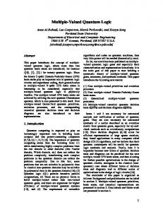
P∞ Then βj (x) = u(x − jh) and j=−∞ βj (x) = 1. The overlaping subsets (Oj ) covering the line are visualised in Fig.(B1).

betaj j= 1

1

j= 2

j= 3

2h

j= 4

j= 5

4h

6h

x

Fig.B1: The functions βj (x) = u(x − jh) decomposing unity.

Each individual βj vanishes with all its derivatives outside (Oj ). Due to the independence of the OPVD functional on the construction of the partition of unity there is no need to consider more elaborate constructions in terms of the constituants functions {uj }. From the relation u(x − jh) + u((j + 1)h − x)) = 1 for x ∈ [jh, (j + 1)h] it follows also that Z (j+1)h γj (k) = dx u(x − jh) e−ikx (B.1)

istic function {χj,h (x) = 1 if jh ≤ x ≤ (j + 1)h, 0 elsewhere }, with the function ρǫ (x) such that ρǫ (x) = (j,h) 1 x (x) 6= 0 for x ∈ [jh − ǫ, (j + ǫ ρ( ǫ ). One has uǫ (j,h) 1)h + ǫ] and uǫ (x) = 1 for x ∈ [jh + ǫ, (j + 1)h − ǫ]. PN −1 (j,h) Then j=0 uǫ (x) is a partition of unity on Ω = [0, L] with L = N h. Another useful construction is achieved, for any ν > 0, with

(j−1)h

= 0

if

2nπ k= , h

h if

k = 0,

∀j.

This orthogonality property leads to the Fourier mode analysis in the distributional context. It is also interesting to note that the orthogonal Bloch functions approach used in the noncompact lattice formulation of gauge theories of Ref.[39] can be then rephrased in terms of the decompositon of unity, the lump functions there being particular realisations of the u(x − jh) with only a finite number of derivatives vanishing outside (Oj ). For completness we give explicitely two constructions of the elementary function u. They are based on the regularising function of L. Schwartz [18] 1

ρ(x) = N e x2 −1

if

|x| < 1,

0

if

|x| ≥ 1,

(B.2) (j,h)

where N stems from normalising ρ(x) to unity. uǫ (x) is then obtained from the convolution of the character-

u(x − jh) =

      

N 0

Rh

2ν

h dv exp[− vν (h−v) ν ], for (j − 1)h < x < (j + 1)h;

|x−jh|

for |x − jh| ≥ h,

(B.3) Rh h2ν where N = 0 dv exp[− vν (h−v) ]. It is verified that for ν any x ∈ [jh, (j + 1)h] one has indeed u(x − jh) + u((j + 1)h − x)) = 1 and that βj vanishes with all its derivatives outside (Oj ) = [(j − 1)h, (j + 1)h]. In the scaled variable kXk the final test function f (X) ≡ f > (X) built in this way is then  (1 − χ(kXk + 1, h))   1 f (X) ≡ f > (X) =   χ(kXk, h) 0

for for for for

0 < kXk ≤ h h < kXk ≤ 1 1 < kXk < 1 + h kXk ≥ 1 + h (B.4)

18

f

f

1

1

1

3

5

X

1

2

3

4

X

Fig.B2: The function f (X) from Eqs.(B4) and from u(x − jh) with ν = 1 a)left curves α = 0.95, dashed: µ2 = 1.25; full line: µ2 = 1.15; b)right curves µ2 = 1.15, dashed: α = 0.95; full line: α = 0.85;

Hence the function χ(kXk, h) is just the very end part of the elementary function u building up unity, say u(kXk − 1) in the last example. Since f (X) vanishes with all its derivatives at kXk = 1 + h, Lagrange’s formula, Eq.(IV.5), is identically fulfilled. Moreover from its construction f (Xt) is different from zero if kXkt < (1 + h). Hence the upper limit of the t-integral in Eq.(IV.5) is tmax = (1+h) kXk . Due to the regularising exponential at the upper boundary it is easily seen on the two constructions presented above that f (X) still vanishes at an kXk-dependant upper boundary with all its derivatives and faster than any inverse power of kXk. This property is assumed to be preserved for the generic function χ(kXk, h(kXk)). One writes now h(X) = µ2 kXkg(kXk) − 1 where µ is an arbitrary dimensionless parameter extracted from g(kXk). It controls then the size of the overlapping regions for two consecutives (Oj ).This is shown in Fig.(B2),where f (X), constructed from Eqs.(B4) and from u(x − jh) with h(X) = µ2 kXkα − 1, is shown respectively at fixed α(viz .µ2 ) for two values of µ2 (viz .α). With the scale in the X variable used in Fig.(B2) for 0 < kXk ≤ h f (X) rises so sharply to 1 that it is not distinguishable from a θ−function. From the discussion in Section IV µ > 1 and 2 (α−1) tmax = (1+h) = µ kXk > 1. The maximum kXk

APPENDIX C: EVALUATION OF LOOP-CONTRIBUTIONS WITH PARTITION OF UNITY TEST FUNCTIONS.

We consider first the one-loop contribution I(k 2 ) to the four-point function of Φ4 scalar field theory at D = 4. We shall work in Euclidean metric to simplify the derivation. I(k 2 ) reads Z 4 f 2 (p2 )f 2 ((p + k)2 ) d p 2 , (C.1) I(k ) = 4 2 (2π) (p + m2 )((p + k)2 + m2 ) Z 1 Z 4 d q f 2 ((q + xk)2 ))f 2 ((q − (1 − x)k)2 ) . = dx (2π)4 (q 2 + k 2 x(1 − x) + m2 )2 0 The two cases k 2 = 0 and k 2 6= 0 must be distinguished. 2 In the first case, with X = Λp 2 , one has I(0) = With T (X) =

Λ4 (4π)2

2 w( Xt ) = θ( kXk − h( kXk t t )) = θ(t − kXk(µ − 1)). Since the extension of T (X) is seeked in the IR and µ ˜ = (µ2 − 1) > 0, µ ˜kXk < 1 is a lower bound to the t-integral in Eq.(IV.3).

0

∞

XdXf 4 (X) . (XΛ2 + m2 )2

(C.2)

1 X.

Hence d =

X lim T (X) (XΛ2 +m2 )2 , X→∞

1, ω = 0, k = 0 and then

1

value of kXk is (µ2 )( 1−α ) and tends to infinity when α tends to 1. For a distribution T (X) singular at the origin of IR d and with the representation of Eq.(B.3) the test function f < (X) behaves simply as w(X) = u(h − kXk) for kXk ≤ h. Then in the limit h → 0 w(X) tends to a step function θ(kXk − h). When α → 1 h effectively tends to zero for values of kXk of the order of µ12 and then

Z

Te(X) = ∂X [

∼

2Xm2 X2 ]= 2 2 +m ) (XΛ2 + m2 )3

(XΛ2

(C.3)

It follows that

2m2 Λ4 (4π)2

Z

∞

Z

µ2

1 dt log(µ2 ) = t (4π)2 0 1 (C.4) In the second case, k 2 6= 0, since the test function is unity for small values of its argument, in the UV regime xkkk and (1 − x)kkk can be disregarded with respect to kqk and the regulation of I(k 2 ) is provided by f 4 (q 2 ) only (This can be checked explicitely by Taylor expansion of I(0) =

XdX (XΛ2 + m2 )3

19 the f ’s, for in all explicitely finite contributions the limit α → 1 can be taken, then f → 1 everywhere and all terms involving derivatives of f with respect to q 2 do not contribute). Eq.(C.1) transforms to I(k 2 ) = =

Λ4 (4π)2 m4

Z

Λ4 (4π)2 m4

Z

1

dx

Z

Xmax

dX

0

0 1

dx

Z

Ymax

dY

(X

Λ2 m2

2

k Y f 4 [Y ( m 2 x(1 − x) + 1)]

(Y

0

0

Xf 4 (X) , k2 2 +m 2 x(1 − x) + 1) Λ2 m2

+ 1)2

(C.5) where, in the last equation, X has been changed to k2 Y (m 2 x(1 − x) + 1). As before d = 1, ω = 0, k = 0 and I(k 2 ) reads now I(k 2 ) =

Z 1 Z Ymax 2Λ4 Y dY dx 2 2 4 Λ (4π) m 0 (Y m2 + 1)3 0 Z ∞ k2 dt 4 (C.6) f [Y t( 2 x(1 − x) + 1)] t m 1

As expected this is another example that the infinite contributions in 2ǫ present in the conventionnal formulation has been removed and replaced by the scale dependance originating from the overlapping domains building up the partition of unity. In a regularisation procedure Λ2 by a cut-off the divergence is log( m 2 ) and, according to Eq.(IV.15), the regulator mass is Λ = µm, hence the final result in log(µ2 ). Instead of the derivation retained here one may use as well Schwinger’s representation for the propagators. The test functions in this case just provide the necessary handling of divergences of the final integrals over Schwinger’s parameter, with the very same result of Eq.(C.7).The way the regularisation works is most simply seen for ∆(0) at D = 4. One has Z

d4 q f (q 2 ) (C.9) (2π)4 q 2 + m2 Z ∞ Z ∞ Λ2 Λ4 du −u y −y m 2 = e f ( ). ydye 2 2 (4π) m 0 u2 u 0

∆(0) =

As discussed in Appendix B the test function effectively 2 in the cuts the t-integration such that t ≤ k2 µ ( m2 x(1−x)+1)

limit α → 1, where Ymax → ∞ and the test function tends to unity over the whole integration domain in Y . Hence 1 I(k ) = (4π)2 2

=

Z

0

1

dx

Z

µ2 2 ( k 2 x(1−x)+1) m

1

1 {log(µ2 ) − (4π)2

Z

1

dx log[ 0

dt t

(C.7)

Now for a SRTF it holds that

k2 x(1 − x) + 1]}. m2

¿From the analysis in dimension D = 4 − ǫ the result is known to be [7] Z Γ(ǫ/2) −ǫ/2 1 k 2 m dx[ 2 x(1 − x) + 1]−ǫ/2 (C.8) (4π)2 m 0 Z 1 1 2 k2 = { x(1 − x) + 1]} + Cte. − dx log[ (4π)2 ǫ m2 0

I(k 2 ) =

Z

∞

yt dt(1 − t)∂t2 tf ( ) u 1 Z ∞ yt dt (1 − t)∂u2 f ( ). = −u2 t u 1

y f( ) = − u

Hence the test function takes care of the divergence at u = 0, and after partial integrations all integrals are now finite giving the result of Eq. (IV.9). We examplify now the general handling of loop contributions with Schwinger’s parametrization for the two-point function Γ2 [k] with two loops. It reads

Z

f 2 (q12 )f 2 (q22 )f 2 ((q1 + q2 − k)2 ) d4 q1 d4 q2 (2π)8 (q12 + m2 )(q22 + m2 )((q1 + q2 − k)2 + m2 ) Z 4 4 4 d q1 d q2 d q3 δ(q3 + k − q1 − q2 )f 2 (q12 )f 2 (q22 )f 2 (q32 ) = (2π)8 (q12 + m2 )(q22 + m2 )(q32 + m2 ) Z Z 3 Y d4 qi −iqi .y f 2 (qi2 ) = d4 yeik.y e (2π)4 (qi2 + m2 ) i=1 Z Z 3 Z Y 2 d4 qi −αi qi2 −iqi .y 2 2 e f (qi ). = d4 yeik.y dαi e−αi m (2π)4 i=1

Γ2 [k] =

(C.10)

In the last relation f 2 (qi2 ) depends in fact only upon the

argument Xi =

qi2 Λ2 .

(C.11)

Then with the change of integration

20 variable αi qi2 → qei 2 the argument of the test function 2 becomes αqeiiΛ2 which implies (cf Appendix B) αi Λ2 > 1 µ2 . The integrals over αi have a lower boundary cutoff at µ21Λ2 , just as in the conventionnal treatment [26]. However using instead Lagrange’s formula for the test functions gives a finite result, whose dependence on the scale parameter µ can be inferred from the conventionnal analysis with the replacement Λ → µm.

It is easy to check that an equivalent representation of f (p) is

f > (p) ≡ −(k + 1)

X Z

|β|=k+1

APPENDIX D: RECOLLECTION OF LAGRANGE’S TYPES OF INTEGRAL FORMULAE FOR SUPER-REGULAR TEST FUNCTIONS.

In this section we collect integral formulae used alternatively in the UV and IR regimes at different places in the main text and show their equivalence. The first one encountered in the IR is given in Eq.(IV.1). At D = 1, after k partial integrations, the following identity also holds for SRTF Z 1 ∞ dk+1 f (X) = − du(X − u)k k+1 f (u) k! X du , Z X k+1 ∞ k+1 =− f (Xt). dt(1 − t)k ∂(Xt) k! 1 Transcribed to arbitrary dimension and with X = p this takes the form X pβ Z ∞ β dt(1 − t)k ∂(pt) f (pt) . f (p) ≡ −(k + 1) β! 1 |β|=k+1

(D.1)

∞

dt

1

(1 − t)k β pβ > f (pt) . ∂(p) (1−d) β! t

(D.2) Here d = D − 1. The same restriction as discussed earlier applies to the t-integral. After partial integration in the UV-extension of T (X) and in the limit α → 1 the upper limit in the t-integration is just µ2 . The Fourier transform φ(x) to the conventionnal x-space representation gives an alternative interpretation of Lagrange’s formula, Eq.(IV.1), valid in the IR. Normalising the Fourierintegral with (2π)(D/2) and after the change of integration variable t → 1/t it reads

φ(x) = (k + 1)

X xβ Z

|β|=k+1

β!

1

dt 0

(1 − t)k β ∂ φ(xt) }, t(k+1) (xt)

(D.3) which is Eq.(IV.1). However when used in the analysis of a distribution singular in the IR and in the limit α → 1 the lower limit in the t-integration comes from the upper limit in the original p-integral and is now just µ12 . With this interpretation Eq.(IV.1) is particularly useful in establishing generalized dispersion-type relations for causal distributions in relation with the findings of [4].