quantum information with optical continuous variables - QuIC

QUANTUM INFORMATION WITH OPTICAL CONTINUOUS VARIABLES: Nonlocality, Entanglement, and Error Correction

Julien Niset Thèse présentée en vue de l’obtention du grade de Docteur en Sciences Appliquées Année Académique 2007-2008

Promoteur: Nicolas Cerf Centre for Quantum Information and Communication

Université Libre de Bruxelles

Faculté des Sciences Appliquées

ii

Acknowledgments

My gratitude goes to Nicolas Cerf for introducing me to the fascinating field of quantum information, and for giving me the opportunity to pursue this thesis. I would also like to thank all of my colleagues at the QuIC, in particular Lo¨ıck Magnin who read a preliminary version of this manuscript, and Louis-Philippe Lamoureux who has become a true friend. Some of the results of this dissertation come from fruitful collaborations. I am very grateful to Antonio Ac´ın and his group at the Institute of Photonic Sciences of Barcelona. My two visits at the ICFO provided me with both inspiration and Sun. I am also grateful to Ulrik L. Andersen of the Technical University of Denmark for his great expertise in quantum optics and outstanding experimental skills. Finally, I would like to thank Jaromir Fiur´ aˇsek of the University of Palack´ y for always finding time to answer my questions. To my friends, to my family, to Veronika.

iii

iv

Contents

1 Introduction

1

2 All you Need to Know About... 2.1 Quantum Mechanics . . . . . . . . . . . . . . . . . . . . . . . 2.1.1 The postulates of Quantum Mechanics . . . . . . . . . 2.1.2 Quantum Mechanics and Impossibilities . . . . . . . . 2.1.3 Entanglement . . . . . . . . . . . . . . . . . . . . . . . 2.2 Quantum Optics . . . . . . . . . . . . . . . . . . . . . . . . . 2.2.1 Quantization of the Electromagnetic Field . . . . . . . 2.2.2 The Quadratures Operators . . . . . . . . . . . . . . . 2.2.3 Representations of the Field . . . . . . . . . . . . . . . 2.2.4 Phase Space Representation and the Wigner Function 2.2.5 Gaussian States . . . . . . . . . . . . . . . . . . . . . . 2.2.6 Gaussian Operations . . . . . . . . . . . . . . . . . . . 2.2.7 Homodyne Detection . . . . . . . . . . . . . . . . . . . 2.3 Information Theory . . . . . . . . . . . . . . . . . . . . . . . 2.3.1 Classical Information Theory . . . . . . . . . . . . . . 2.3.2 Quantum Information Theory . . . . . . . . . . . . . .

9 10 10 13 17 19 20 20 21 24 26 29 31 33 33 35

3 Testing Quantum Nonlocality 3.1 Introduction . . . . . . . . . . . . . . . . . . . . . . . . 3.2 Bell Tests and Related Loopholes . . . . . . . . . . . . 3.2.1 The CHSH inequality . . . . . . . . . . . . . . 3.2.2 Detector Efficiency and Locality Loophole . . . 3.3 Bell Tests and Continuous Variables . . . . . . . . . . 3.3.1 Bell Tests Based on Quadrature Measurements 3.3.2 Multimode Nonlocality . . . . . . . . . . . . .

37 37 39 39 41 42 42 43

v

. . . . . . .

. . . . . . .

. . . . . . .

. . . . . . .

3.4

3.5 3.6

Multimode Nonlocality using Homodyne Detection . . . . 3.4.1 Correlated Photon Number states . . . . . . . . . 3.4.2 Maximal Violation . . . . . . . . . . . . . . . . . . 3.4.3 Noise Effects . . . . . . . . . . . . . . . . . . . . . A Three-Partite Candidate for a Loophole Free Bell Test . Conclusion . . . . . . . . . . . . . . . . . . . . . . . . . .

4 Nonlocality without Entanglement 4.1 Introduction . . . . . . . . . . . . . . . . . . 4.2 The Domino States . . . . . . . . . . . . . . 4.3 The Asymmetry of Local Distinguishability 4.4 The SHIFT Ensemble . . . . . . . . . . . . 4.4.1 A Circuit Based Picture . . . . . . . 4.4.2 Understanding the Circuit . . . . . . 4.5 Multipartite NLWE in arbitrary dimension 4.5.1 More Parties and More Dimensions . 4.5.2 A Lengthy but Generic Proof . . . . 4.5.3 Concluding Remark . . . . . . . . . 4.6 From Discrete to Continuous Variables . . . 4.6.1 Unphysical Proof of Principle . . . . 4.6.2 Unproved Physical Example . . . . . 4.7 Conclusions . . . . . . . . . . . . . . . . . .

. . . . . . . . . . . . . .

. . . . . . . . . . . . . .

. . . . . . . . . . . . . .

. . . . . . . . . . . . . .

. . . . . . . . . . . . . .

. . . . . . . . . . . . . .

. . . . . . . . . . . . . .

. . . . . . . . . . . . . .

. . . . . .

. . . . . . . . . . . . . .

. . . . . .

44 45 50 53 55 58

. . . . . . . . . . . . . .

61 61 63 64 65 65 68 69 69 70 73 74 75 77 78

5 Nonlocality Without Squeezing 5.1 Introduction . . . . . . . . . . . . . . . . . . . . . . . . . . . . 5.2 Parallel and Antiparallel Spins . . . . . . . . . . . . . . . . . 5.3 Spin Flipping and Phase Conjugation . . . . . . . . . . . . . 5.4 Superiority of Entangled Measurement over All Local Strategies 5.4.1 The Optimal Local Fidelity for |αi |α∗ i and |αi |αi Are Equal . . . . . . . . . . . . . . . . . . . . . . . . . . . 5.4.2 The Optimal Measure-and-Prepare Strategy on |αi|αi is Local . . . . . . . . . . . . . . . . . . . . . . . . . . 5.4.3 A Better Measurement on Phase-Conjugate Coherent States . . . . . . . . . . . . . . . . . . . . . . . . . . . 5.5 Experimental Demonstration . . . . . . . . . . . . . . . . . . 5.5.1 Sideband Encoding . . . . . . . . . . . . . . . . . . . . 5.5.2 The Setup . . . . . . . . . . . . . . . . . . . . . . . . . 5.5.3 Local Measurement Strategy . . . . . . . . . . . . . . 5.5.4 Joint Measurement Strategy . . . . . . . . . . . . . . . 5.6 Conclusion . . . . . . . . . . . . . . . . . . . . . . . . . . . . vi

81 81 83 84 86 87 88 90 93 93 94 95 96 97

6 Gaussian Error Correction 6.1 Introduction . . . . . . . . . . . . . . . . . . . . . . . . 6.2 Preliminaries . . . . . . . . . . . . . . . . . . . . . . . 6.3 On the Impossibility of Gaussian Error Correction . . 6.3.1 Error Correction and Entanglement Distillation 6.3.2 Entanglement Degradation of a Channel . . . . 6.3.3 A No-Go theorem . . . . . . . . . . . . . . . . 6.4 Applications . . . . . . . . . . . . . . . . . . . . . . . . 6.4.1 Important Examples of Gaussian Channels . . 6.4.2 Quantum Capacity . . . . . . . . . . . . . . . . 6.5 Conclusion . . . . . . . . . . . . . . . . . . . . . . . . 7 Experimentally Feasible Quantum ECC 7.1 Introduction . . . . . . . . . . . . . . . . . . . . . . 7.2 An Erasure Correcting Code for Discrete Variables 7.3 A Deterministic Protocol: Erasure Correction . . . 7.3.1 The Optical Setup . . . . . . . . . . . . . . 7.3.2 Performances . . . . . . . . . . . . . . . . . 7.3.3 Comments . . . . . . . . . . . . . . . . . . . 7.4 A Probabilistic Protocol: Erasure Filtration . . . . 7.4.1 From Feedforward to Postselection . . . . . 7.4.2 Evaluating the Performances . . . . . . . . 7.4.3 Results . . . . . . . . . . . . . . . . . . . . 7.4.4 A Simpler Setup . . . . . . . . . . . . . . . 7.5 Experimental Realization . . . . . . . . . . . . . . 7.6 Conclusion . . . . . . . . . . . . . . . . . . . . . . 8 Conclusion

. . . . . . . . . . . . .

. . . . . . . . . . . . .

. . . . . . . . . .

. . . . . . . . . . . . .

. . . . . . . . . .

. . . . . . . . . . . . .

99 99 100 102 102 104 108 108 108 109 110

. . . . . . . . . .

. . . . . . . . . .

. . . . . . . . . . . . .

113 . 113 . 114 . 115 . 115 . 117 . 119 . 120 . 120 . 121 . 123 . 126 . 126 . 128 131

A N-Partite Unextendible Product Bases 139 A.1 From Nonlocality Without Entanglement to Unextendible Product Bases . . . . . . . . . . . . . . . . . . . . . . . . . . . . . 139 A.2 Examples . . . . . . . . . . . . . . . . . . . . . . . . . . . . . 140 B N-partite Bound Entangled States

143

C CV Secret Sharing

147

D Manipulating Wigner functions 149 D.1 Partial Trace . . . . . . . . . . . . . . . . . . . . . . . . . . . 149 D.2 Conditional measurement . . . . . . . . . . . . . . . . . . . . 150 D.3 Single-mode Fidelity . . . . . . . . . . . . . . . . . . . . . . . 151 vii

E Entanglement Distillation E.1 Introduction . . . . . . . E.2 Optical Setup . . . . . . E.3 Performances . . . . . . E.4 Conclusion . . . . . . .

. . . .

. . . .

. . . .

viii

. . . .

. . . .

. . . .

. . . .

. . . .

. . . .

. . . .

. . . .

. . . .

. . . .

. . . .

. . . .

. . . .

. . . .

. . . .

. . . .

. . . .

. . . .

153 153 154 155 157

List of Figures

2.1 2.2 2.3 2.4

Phase-space representation of some Gaussian states . . . . Decomposition of an arbitrary symplectic transformation Schematic of an ideal homodyne detection . . . . . . . . . Venn diagram . . . . . . . . . . . . . . . . . . . . . . . . .

. . . .

. . . .

28 31 32 35

3.1 3.2 3.3 3.4 3.5

Schematic of a Bell test with two parties and two settings Coefficients cn for the optimal state: m = 3, d = 20 . . . . Coefficients cn for the optimal state: m = 2, d = 30 . . . . Bell factor B3 for the state |Ψ′3 i . . . . . . . . . . . . . . . Conditional generation of the state |Ψ′3 i . . . . . . . . . .

. . . . .

. . . . .

41 48 49 57 58

4.1 4.2

Graphical depiction of the domino states . . . . . . . . . . . . Quantum circuit generating the SHIFT ensemble from the computational basis . . . . . . . . . . . . . . . . . . . . . . . Minimum classical communication to enable local distinguishability . . . . . . . . . . . . . . . . . . . . . . . . . . . . . . . . Nonlocality without entanglement in 3 ⊗ 3 ⊗ 3 ⊗ 3 . . . . . . Additional quantum circuit for NLWE in 3 ⊗ 3 ⊗ 3 ⊗ 3 . . . .

64

4.3 4.4 4.5 5.1 5.2

67 69 71 74

5.3 5.4

The Phase conjugation operator . . . . . . . . . . . . . . . . . Optimal measure-and-prepare strategy for the discrimination of |αi |αi and |αi |α∗ i . . . . . . . . . . . . . . . . . . . . . . Schematic of the experimental setup . . . . . . . . . . . . . . Spectral power densities of the local and joint strategies . . .

6.1 6.2

Schematic of a Gaussian error correction protocol . . . . . . . 101 From a GECC to a Gaussian Entanglement Distillation protocol103 ix

85 91 95 96

LIST OF FIGURES 7.1 7.2 7.3 7.4 7.5 7.6 7.7 7.8 7.9

Encoding circuit for the qubit erasure-correcting code . . . . Encoding circuit for the CV quantum erasure-correcting code Decoding circuit for the correction of one erasure . . . . . . . Fidelity (7.14) of the erasure correcting code as a function of the squeezing factor of the two-mode squeezed state . . . . . Schematic of the Erasure Filter . . . . . . . . . . . . . . . . . Fidelity and success probability of the erasure-filter versus the erasure probability for various degrees of squeezing . . . . Fidelity of the erasure-filter versus the erasure probability for various intensity of the first and second input states . . . . . Simple setup to improve the transmission of coherent states over the erasure channel . . . . . . . . . . . . . . . . . . . . . Fidelity and success probability of the simplified erasure-filter versus the erasure probability for various intensity of the input state . . . . . . . . . . . . . . . . . . . . . . . . . . . . . .

115 116 118 119 121 123 125 126

127

A.1 Representation of an unextendible product bases and the associated bound entangled state . . . . . . . . . . . . . . . . . 140 E.1 Experimentally feasible distillation protocol . . . . . . . . . . 154 E.2 Experimentally feasible distillation protocol, a simpler version 155 E.3 Performances of the (4 → 2)-entanglement distillation protocol for various degrees of entanglement of the input two-mode squeezed vacuum . . . . . . . . . . . . . . . . . . . . . . . . . 156

x

1 Introduction Information is (Quantum) Physical The 20th century will be remembered, without a doubt, as a century of great technological discoveries. Remarkably, many of these new technologies find their roots in two mathematical theories which completely revolutionized our perception of the world we live in. In 1901, in an attempt to explain the black-body radiation, Max Planck suggested that the energy of the emitted radiation could be described as consisting of discrete packets or quantas [87]. His remarkable intuition was soon embraced by Albert Einstein who used this idea of quantization to explain the photoelectric effect [32], and the specific heat of solids at very low temperature [33]. The quantum revolution was on its way. Since its introduction, this theory of the infinitely small has found applications ranging from the invention of the laser to the discovery of superconductivity. Forty-seven years and two world wars later, the need for efficient communication protocols led Claude Shannon to publish an article entitled “A Mathematical Theory of Communication” [92]. In this seminal paper, a collection of unpublished results gathered during the war, he addressed the problem of the transmission of information over noisy channels by introducing new mathematical objects such as the entropy of a probability distribution or the capacity of a communication channel. The resulting theory, known as Information theory, radically changed our modern society by providing a mathematical framework for the development of information oriented applications such as the computer, the compact-disk, the internet, i.e. all applications we now label as information technologies (IT). 1

CHAPTER 1. Introduction Interestingly, these two theories, which emerged in different contexts and address different issues, are not as far apart as they seem. On the one hand, information needs a physical support to be transmitted. When we speak, the surrounding molecules of air vibrate according to the sounds we make. The words I am typing now are stored in the hard drive of my computer, and will later be printed on a piece of paper. To quote Rolf Landauer, “Information is physical” [70]. On the other hand, physical objects are, ultimately, made of microscopic particles described by the laws of quantum theory. A bit of information stored on my computer is nothing but a collection of millions of electrons, where each and everyone obey the laws of quantum mechanics. Information should not only be physical then, but quantum physical! Just as classical mechanics is an approximation of quantum mechanics valid for macroscopic objects, the information theory developed by Shannon should be the classical approximation of a quantum information theory which applies when information is stored and manipulated on quantum mechanical systems. At the dawn of the 70’s, exploring the possibilities and implications of this quantum version of information theory rapidly gained interest among a small group of pioneer physicists such as Richard Feynman, Charles Bennett, Paul Benioff, and David Deutsch. A new revolution was about to begin. But let us not go too fast. In parallel of these intellectual considerations, the 60’s also witnessed the rise of the computer era. Since the first integration of a transistor in an electronic circuit in 1958, the performances of computing machines had been improving at an amazing pace. This led Gordon Moore, a co-founder of Intel, to conjecture in 1965 that the number of transistors one can place on an integrated circuit was to increase exponentially, approximately doubling every two years [75]. Amazingly enough, his predictions have held true for more than 40 years! However, people soon realized that such a trend could not continue for ever as the size of transistors would ultimately have to reach the size of atoms and enter the quantum regime. As noted by Moore himself in 2005, “It can’t continue forever. The nature of exponentials is that you push them out and eventually disaster happens”. But is a disaster due to the extreme miniaturization of transistors inevitable? Probably not if one is willing to seriously investigate the capabilities of this extreme quantum regime of computation. At the beginning of the 80’s, both intellectual and economical motivations were present for the rapid development of a new fascinating field of research; Quantum Information Science (QIS) was born. The promises of Quantum Information How can one benefit from the association of quantum mechanics with Shannon’s theory of information? At first sight, the use of microscopic objects to support information seems to be the source of more problems than solutions. 2

For example, Heisenberg’s uncertainty principle predicts the impossibility to obtain all the information about the spin of a single particle. How can two parties, say Alice and Bob, exchange information if they are unable to read the messages they receive? Interestingly, it is precisely this impossibility to read unknown quantum information which led Stephen Wiesner, then a graduate student at Columbia, to what is considered as the first application of quantum information theory; namely quantum money [105] (ironically, Wiesner proposed this idea in 1970, but had to wait until 1983 to publish it). By integrating a series of two-level quantum systems on a bank note, Wiesner argued that it is possible to create an unforgeable note whose security is guaranteed by the laws of quantum mechanics. Indeed, preparing these systems in well defined non-orthogonal quantum states would force a counterfeiter to measure each of them in a random basis, thereby introducing perturbations in the copies which could be easily detected by the bank. This unpractical but brilliant idea led, a few years later, to the discovery of quantum key distribution [8] and is at the origin of an entire branch of QIS devoted to cryptographic applications and communications. Asides from the uncertainty principle, quantum mechanics has some other interesting fundamental features with no classical counterparts. Can they be exploited cleverly in order to solve, say, computational problems efficiently? This question was first addressed by David Deutsch, who suggested that, indeed, such quantum computers might have a computational power exceeding that of classical ones [28]. Consider for example a bit, the basic unit of classical information, which has only two possible values “0” or “1”. Either a million electrons are stored in a given memory cell of my computer and the bit is interpreted as “one”, or they are not and the bit is interpreted as “zero”. Now suppose that this memory cell is a two-level quantum system such as the spin of a single electron. The superposition principle of quantum mechanics predicts that this quantum bit, or qubit, can not only be |0i or |1i, but can also be |0i and |1i at the same time, i.e. quantum mechanics enables linear superpositions of the form |ψi = α |0i + β |1i. By processing this qubit, one will therefore process “zero” and “one” simultaneously, a feature of quantum computation known as parallelism. In 1994, these considerations led Peter Shor to design an efficient algorithm, the so-called Shor algorithm, proving the superiority of quantum over classical computers for the factorization of large numbers [93]. Interestingly, while the uncertainty principle guarantees the security of specific cryptographic tasks, the superposition principle enables parallel quantum computation and is at the origin of the computation and algorithmic branch of QIS. The power of quantum information lies in its ability to exploit the many possibilities offered by the quantum world. Its development is therefore strongly correlated to our knowledge and understanding of quantum mechanics. Remarkably, the rise of quantum information caused a renewed interest in the foundations of this well established theory. Questions which 3

CHAPTER 1. Introduction were left unanswered or considered uninteresting for nearly a century soon became the focus of intensive research. The most striking example of this renewal is a property of quantum mechanics known as entanglement. The term entanglement was first coined by Erwin Schr¨ odinger as “the characteristic trait of quantum mechanics” [91]. It was also called “spooky action at the distance” by Albert Einstein, and its implications caused Einstein to dislike the theory he had helped create. He was not the only one puzzled by such a counterintuitive aspect of quantum theory, although for many years questions related to entanglement were mostly considered of philosophical and metaphysical nature. Following the work of John Bell [7], the recent renewal of quantum mechanics has seen our understanding of entanglement change from a controversial property of microscopic entities to a key ressource of quantum information. Entanglement is now used to achieve many tasks such as quantum teleportation [9] or quantum dense coding [10]. An entire branch of QIS, sometimes known as entanglement theory, is now devoted to the study of this fascinating ressource, ranging from its characterization to the exploration of its possible uses. Continuous Variables The early investigations of quantum information mostly focused on qubits, i.e. two-level quantum systems such as the spin of an electron or the polarization of a photon, since they are the natural quantum analog of the classical bit. From a theorist’s perspective, these systems are the simplest to manipulate. They also exhibit all the quantum features interesting for quantum information applications. Using qubits, quantum states can be teleported, secret keys can be established, numbers can be factorized, entanglement can be produced, distributed and distilled. Unfortunately, manipulating a single photon (or a single electron) is a difficult experimental task. Single photons are hard to produce on demand, and hard to detect efficiently. The same applies to the production and detection of entanglement. These experimental limitations make the implementation of quantum information based on discrete variables both difficult and expensive. Since 1998, the year of the first experimental demonstration of unconditional quantum teleportation by Furusawa and collaborators [43], a novel approach developed, which relies on canonical observables with continuous spectra. This quantum information with continuous variables (CV) rapidly gained attention as it offers many practical advantages over its discrete variable counterpart. On the one hand, when the quadratures of the electromagnetic field are used to carry the information, many interesting protocols can be implemented by combining passive and active linear optical components (beam splitters, phase shifters and squeezers), supplemented with an efficient detection scheme known as homodyne detection. All these elements are, up to some degree of accuracy, readily accessible in today’s optical labs. 4

Furthermore, continuous variable entangled states of light can be relatively easily generated in a deterministic way with optical parametric amplifiers [20], while their continuous quantum information is made accessible by the fast and efficient homodyne detection technique. On the other hand, although CV states lie in an infinite dimensional Hilbert space, many of them can be handled by mathematical techniques from finite-dimensional algebra. In particular, operations on the density matrix of the so-called Gaussian states can be achieved by manipulating the finite-dimensional covariance matrix. All these features make the optical continuous variable approach a very promising candidate for quantum information and quantum communications in particular. Outline of the Thesis The objective of the present dissertation is to investigate some of the possibilities offered by the continuous variable approach of quantum information, with a focus on optical continuous variables in particular. As often in science, practical applications emerge from purely theoretical considerations. Quantum information is no exception, and many of its remarkable accomplishments are the results of an improved understanding of quantum mechanics and its many mysteries. The first part of this dissertation will therefore be oriented towards fundamental issues. More precisely, we will address various nonlocal aspects of quantum mechanics in the continuous variable regime, and try to gain some insight into the peculiar relation between the two essential ressources of QIS, namely nonlocality and entanglement. The second part of the dissertation will be oriented towards practical applications. In particular, we will focus on an important primitive of quantum information called error correction, and exploit optical continuous variables advantageously in order to design experimentally feasible error-correcting codes. Quantum information is an interdisciplinary field. In Chapter 2, we will introduce some basic concepts and mathematical tools central to quantum mechanics, quantum optics, and information theory. Readers familiar with CV quantum information are free to skip this preliminary chapter. The next three chapters aim to improve our understanding of quantum nonlocality in the continuous variable regime. In Chapter 3, we focus on the standard nonlocality of quantum mechanics, and address the problem of loophole-free Bell inequalities. We will show that Bell tests based on optical continuous variables combined with homodyne detection can benefit from an increased number of parties involved in the experiment. In particular, we will prove that it is always possible to maximally violate the m-partite Mermin-Klyshko inequality based on such quadrature measurements. In Chapter 4, we will generalize a bizarre property of quantum mechanics 5

CHAPTER 1. Introduction known as Nonlocality Without Entanglement (NWE). This peculiar effect, first identified in 1998 for three-level quantum systems, describes systems that behave in a truly nonlocal manner without being entangled. By introducing a simple quantum circuit, we will generalize the phenomena to arbitrary dimension, and investigate the possibility to witness this effect with CV states. Finally, the first part of this dissertation will be concluded by introducing in Chapter 5 a third form of nonlocality arising when certain non-entangled states are detected with an entangled measurement. We will name this property Nonlocality Without Squeezing, and experimentally demonstrate its existence based on phase conjugated coherent states. The second part of the thesis will be devoted to quantum error correction with continuous variables. In Chapter 6, we will exploit a known connection between error correction and entanglement distillation to prove that a large class of CV errors, called Gaussian errors, cannot be corrected using the available Gaussian operations (linear optical elements plus homodyne detection). We will nevertheless show in Chapter 7 that non-Gaussian error patterns can be corrected using Gaussian operations only, and we will present the first continuous-variable quantum erasure-correcting code. The key feature of our code is a nonlocal transmission of information that is made possible by the use of CV entangled states. In Chapter 8, we will summarize our results and look upon future perspectives. Publications This dissertation is based on the following publications: • J. Niset and N. J. Cerf, Multipartite Nonlocality Without Entanglement in Many Dimensions, Phys. Rev. A 74, 052103 (2006). • J. Niset, A. Ac´ın, U. L. Andersen, N. J. Cerf, R. Garc´ıa-Patr´ on, M. Navascués, and M. Sabuncu, Superiority of Entangled Measurements over All Local Strategies for the Estimation of Product Coherent States, Phys. Rev. Lett. 98, 260404 (2007). • J. Niset and N. J. Cerf, Tight Bounds on the Concurrence of Quantum Superpositions, Phys. Rev. A 76, 042328 (2007). • J. Niset, U.L. Andersen, N.J. Cerf, Experimentally Feasible Quantum Erasure-Correcting Code for Continuous Variables, Phys. Rev. Lett. 101, 130503 (2008). • A. Acin, N.J. Cerf, A. Ferraro, and J. Niset, Multimode Quantum NonLocality Using Homodyne Measurements, arXiv:0808.2373 (submitted to Phys. Rev. A). 6

• J. Niset, and N.J. Cerf, A No-Go Theorem for Gaussian Error Correction, in preparation.

7

CHAPTER 1. Introduction

8

2 All you Need to Know About...

This chapter

Quantum information is an interdisciplinary field. Fundamentally, it combines aspects of quantum mechanics, information and computation theory. However, going from theory to experiment also requires knowledges of quantum optics, atomic physics, or solid state physics depending on the physical system used to support the information. Good quantum information theorists must therefore combine expertise of some, if not all, of these different fields. The present dissertation being concerned with quantum information based on optical continuous variables, we will restrict our attention to quantum mechanics, quantum optics, and information theory. Each of these topics is a field on its own; presenting them in a single chapter is therefore a difficult, if not impossible, task. Nevertheless, the following sections are an attempt to introduce the basic concepts and features of these three theories, together with the associated mathematical formalism. Our goal is to provide an unfamiliar reader with the necessary tools to tackle the problems addressed in this thesis. However, a brief introduction can never replace a good book, and we note that this chapter is mainly a compilation of results found in [78, 101, 20, 26]. Interested readers are strongly encouraged to consult these very instructive references for more details and (probably) better explanations. 9

CHAPTER 2. All you Need to Know About...

2.1 2.1.1

Quantum Mechanics The postulates of Quantum Mechanics

The aim of quantum information theory is to use microscopic physical systems to store and manipulate information. These systems can be quite different in nature, but irrespective of their differences they can all be described within a common mathematical framework called quantum mechanics. This is what makes quantum mechanics both beautiful and powerful. Whether we consider the spin of an electron, the polarization of a photon, or the atomic levels of an atom, the mathematical objects we manipulate are the same. In itself, quantum mechanics is not a theory about which laws a particular physical system must obey, but it provides some general principles from which a mathematical description of these laws can be developed. These general principles can be formulated as a set of basic postulates, which we present here in a form that is particularly suitable for quantum information. The first postulate of quantum mechanics defines the mathematical entity representing a particular state of a physical system. Postulate 1 To any isolated physical system S is associated a Hilbert space (a complex vector space with inner product) HS . The system state is completely determined by a unit vector |ψi of that Hilbert space. Remarkably, this postulate does not specify what Hilbert space will be associated to a given physical system, that is, it does not give the basis states or even the dimension of the space HS . In general, this dimension should be adequately chosen to be able to reproduce the physical properties of the system. As we will see, this dimension can be finite or infinite. An important consequence of Postulate 1 is that vectors in a Hilbert space, and therefore quantum states, have the interesting property that if |ψ1 i and |ψ2 i are two states in HS , so will be any linear combination |ψ3 i = α |ψ1 i+β |ψ2 i where α and β are complex numbers such that |α|2 + |β|2 = 1. This property, known as the superposition principle of quantum mechanics, is at the origin of the power of quantum information. Finally, the inner product of two states |ψ1 i and |ψ2 i of HS is denoted by the bracket notation hψ1 |ψ2 i. While the first postulate deals with states at a fixed time, the second postulate tells us how these states evolve in time. Postulate 2 The evolution of an isolated quantum system is described by a unitary transformation. That is, the state |ψ ′ i of the system at time t′ is 10

2.1. Quantum Mechanics related to the state |ψi of the system at time t by ′ ψ = U |ψi ,

(2.1)

where U is a unitary operator which depends on the times t and t′ . Just as quantum mechanics does not tell us the state space or quantum state of a particular physical system, it does not tell us which unitary operator describes its evolution. However, it assures us that this evolution may be described in such a way. From the unitarity of the evolution follows the interesting property that quantum processes are always reversible. In practice, systems are never perfectly isolated as required by this second postulate. Nevertheless, there are interesting systems which can be described to a good approximation as being closed, and whose evolution is approximately unitary. In any case, we note that, at least in principle, every open system can be described as part of a larger closed system, the Universe, which is undergoing a unitary evolution.

So far, the postulates have only considered isolated systems. It is however clear that it is necessary to interact with a system at some point if we want to extract some information from it. The process of interacting with a system to extract information is called a measurement, and is the purpose of the following postulate. Postulate 3 A quantum measurement on a system S is described by a collection {Mm } of measurement operators, defined as operators acting in the Hilbert space HS associated with S and satisfying the completeness relation X † Mm Mm = IS (2.2) m

where IS is the identity operator on HS . The index m refers to the measurement outcomes that may occur in an experiment. The probability p(m) to obtain the outcome m if the system was in the state |ψi immediately before the measurement is given by † p(m) = hψ|Mm Mm |ψi,

(2.3)

and the state after the measurement becomes Mm |ψi p . p(m)

(2.4)

Measurements will play an important role in the following chapters, and are central to quantum information. As we will see, they are often the last step of an experiment where one is only interested in the probabilities of getting 11

CHAPTER 2. All you Need to Know About... the different outcomes. In this case, postulate 3 shows that the only relevant † mathematical entities are the positive operators Em = Mm Mm . The set of operators {Em } is called a Positive Operator-Valued Measure, or POVM in short, and the POVM elements Em satisfy the completeness relation X Em = IS . (2.5) m

Physicists may not be familiar with this formulation of the measurement postulate. In traditional quantum physics, each physical property that can be measured corresponds to a hermitian Poperator M , called an observable, that has a spectral decomposition M = m mPm , where the m’s are the eigenvalues of M and Pm is the projector to the corresponding eigenspace. These projectors Pm , with Pm Pm′ = δmm′ Pm , define a particular type of measurement called projective or von Neumann measurement, and correspond to the special case where the measurement operators Em are orthogonal projectors. Within this notation, we do recover the measurement postulate as stated in most books on quantum mechanics, i.e. the possible outcomes of a measurement are the eigenvalues m of the corresponding observable M , and the state after the measurement lies within the eigenspace of M associated with the observed outcome m. Let us also mention that we will sometimes refer to “measuring in a basis |mi”, where |mi forms an orthogonal basis. This simply means that we perform a projective measurement with projectors Pm = |mihm|. Our generalized formulation of the measurement postulate naturally raises two questions. First, one may wonder why we state the postulate in this form. The answer can be found in the development of quantum information theory, which has showed that it is often possible to extract more information from a system by going beyond projective measurements (see for example Chapter 4). Second, one may question the validity of the measurement postulate in this form. As we now see, this formulation is strictly equivalent to the traditional one provided that we add this last postulate Postulate 4 The Hilbert space associated with a composite physical system AB, made of two subsystems A and B, is the tensor product HA ⊗ HB of the Hilbert spaces HA and HB associated with A and B. Furthermore, if A is prepared in the state |ψA i and B is prepared in the state |ψB i, the joint state of the composite system AB will be the tensor product state |ψA i ⊗ |ψB i, sometimes noted as |ψA i |ψB i for simplicity. Suppose for example that we want to realize the generalized measurement {Mm } on a system S. We can always extend S by adding an additional system A prepared in a known state, and such that the dimension of HA coincides with the number of measurement operators Mm . Associating each Mm with a basis state |mi of A, it is always possible to define a unitary 12

2.1. Quantum Mechanics P operator U such that U |ψi |0i = m Mm |ψi |mi, where |ψi is the unknown state of S and |0i is some arbitrary fixed state of A known as an ancilla. It is now straightforward to check that the generalized measurement {Mm } on S can be realized by a projective measurement on SA with projectors Pm = U † (IS ⊗ |mihm|)U , where IS is the identity on HS and |mihm| is the projector on the state |mi of HA . This useful correspondence between POVMs and projective measurements in a larger system is known in quantum information as Neumark’s theorem [86]. So far, we have formulated quantum mechanics using the language of state vectors. However, it is important to note that there exists an alternate formulation using a tool known as the density operator. This formulation is mathematically equivalent, but much more practical in some commonly encountered scenarios in quantum mechanics. In particular, the density operator provides a convenient means for describing quantum systems whose state is not completely known. For example, if a quantum system can be in one of the states {|ψi i} with respectives probabilities pi , the state of the system is fully characterized by the density operator ρ≡

X i

pi |ψi ihψi |.

(2.6)

A quantum system whose state |ψi is known exactly is said to be pure, and its density operator is simply ρ = |ψihψ|. Otherwise, the state is said to be mixed and the density operator has the form of Eq. (2.6). Both formulations will be used interchangeably in the following chapters, and we refer the reader to e.g. [78] for some important properties of the density operator.

2.1.2

Quantum Mechanics and Impossibilities

Remarkably, the simple formalism introduced by these four postulates is sufficient to derive some interesting properties of the quantum theory. For example, it can tell us what is possible and impossible within the framework of quantum mechanics. Interestingly, this is exactly the goal of quantum information; to test the possibilities offered by quantum mechanical systems and see what it implies for the treatment of information. In the following section, we thus present three limitations imposed by quantum mechanics that have been of fundamental importance in the development of QIS. These impossibilities will help us grasp the flavor of the revolutionary concepts introduced by quantum mechanics. They will also introduce the principles which triggered most of the questions addressed in this dissertation. 13

CHAPTER 2. All you Need to Know About... Distinguishing Quantum States An important question in quantum information is the problem of distinguishing quantum states. In the classical world, distinct states of an object are usually distinguishable. One can always tell if the result of a coin toss is head or tail for example. In the quantum world however, the situation is more complicated. As we will see in Chapter 4 and 5, it also leads to some very counterintuitive results. The question of the distinguishability of quantum states is best understood by considering the following simple game between two parties usually called Alice and Bob. Suppose that Alice chooses a state |ψi i (1 ≤ i ≤ n) from a given set known to her and Bob, and sends the state to Bob. Bob’s task is to identify the value of the label i. Let us assume first that the states of the set are orthogonal. Bob can define the n measurement operators Mi = |ψi ihψi |, and an additional measureP ment operator M0 = I − i Mi . These operators satisfy the completeness relation, and if the state |ψi i is prepared by Alice then p(i) = hψi | Mi |ψi i = 1 so Bob will identify the index i with certainty. It is thus possible to reliably distinguish orthogonal quantum states. Suppose now that the states of the set are not orthogonal, and let us imagine that there exists a measurement which can distinguish perfectly between the non-orthogonal states |ψ1 i and |ψ2 i. Bob will apply his measurement described by the measurement operators Mj , and if the outcome j is observed, he guesses that the index is i using some rule f (j) = i. If the state |ψ1 i (|ψ2 i) is prepared then the probability of measuring j such that P f (j) = 1 (f (j) = 2) must be one. Introducing Ei = j:f (j)=i Mj† Mj , this translates to hψ1 | E1 |ψ1 i = 1

hψ2 | E2 |ψ2 i = 1. (2.7) P P Since i Ei = I, it follows that i hψ1 | Ei |ψ1 i = 1, and (2.7) implies √ hψ1 | E2 |ψ1 i = 0, or equivalently E2 |ψ1 i = 0. Now, because the two states are not orthogonal, we can write |ψ2 i = α |ψ1 i + β |ϕi , 2 2 where √ |ϕi is orthogonal to |ψ1 i, |α| +|β| = 1 and |β| < 1. Then β E2 |ϕi which implies

hψ2 | E2 |ψ2 i = |β|2 hϕ| E2 |ϕi ≤ |β|2 < 1.

(2.8) √

E2 |ψ2 i = (2.9)

This is in clear contradiction with (2.7), from which we can deduce that there is no quantum measurement capable of distinguishing reliably between nonorthogonal states.

14

2.1. Quantum Mechanics Measuring Non-Commuting Observables In quantum mechanics, a physical property that can be measured, or observed, is associated with an hermitian operator called an observable. Sometimes, these observables correspond to physical properties that are complementary, and the order in which these observables are applied to a state matters. If A and B are two such non-commuting observables, this property is expressed as [A, B] = AB − BA 6= 0,

(2.10)

where [A, B] is called the commutator of A and B (we can also define their anti-commutator {A, B} = AB + BA). In 1926, Werner Heisenberg arrived at the astonishing conclusion that quantum mechanics precludes the perfect knowledge of such non-commuting observables simultaneously. This famous result is known as Heisenberg’s uncertainty principle. Let us consider two non-commuting observables A and B, a quantum state |ψi, and suppose that hψ| AB |ψi = x + iy, where x and y are real. Note that hψ| AB |ψi is called the average value of AB for the state |ψi, and is sometimes denoted as hABi when it is clear that we refer to the state |ψi. We can calculate the average value of the commutator and anti-commutator of AB, hψ| [A, B] |ψi = 2iy

hψ| {A, B} |ψi = 2x,

(2.11)

which implies | hψ| [A, B] |ψi |2 + | hψ| {A, B} |ψi |2 = 4| hψ| AB |ψi |2 .

(2.12)

By the Cauchy-Schwartz inequality, we also know that | hψ| AB |ψi |2 ≤ hψ| A2 |ψi hψ| B 2 |ψi ,

(2.13)

from which we deduce | hψ| [A, B] |ψi |2 ≤ 4| hψ| AB |ψi |2 ≤ 4 hψ| A2 |ψi hψ| B 2 |ψi .

(2.14)

If we now define two new observables C and D such that A = C − hCi and B = D − hDi, we obtain Heisenberg uncertainty principle |h[C, D]i| , (2.15) 2 where we have introduced the standard deviation ∆M of an observable M with ∆C ∆D ≥

∆2 M = h(M − hM i)2 i = hM 2 i − hM i2 . 15

(2.16) (2.17)

CHAPTER 2. All you Need to Know About... The conceptual implications of this uncertainty principle are at the origin of the discussion of the standard nonlocality of quantum mechanics addressed in Chapter 3. Copying Quantum States Quantum information is carried by quantum states. Unlike classical information, quantum information is not easy to manipulate as it requires the manipulation of quantum objects. For example, a simple task such as perfectly copying an unknown quantum state is precluded by the laws of quantum mechanics. This principle, known as the no-cloning theorem, is at the origin of the most advanced application of quantum information called Quantum Key Distribution. Suppose that we have at hand a device which can copy an arbitrary quantum state. In particular, it can copy the two orthogonal states |ψi and |ψ⊥ i. Without loss of generality, we can associate to our device a unitary operator U acting on the state we want to copy and the “blank” ancilla to which we want the copied state, i.e. U |ψi |0i = |ψi |ψi

U |ψ⊥ i |0i = |ψ⊥ i |ψ⊥ i

(2.18) (2.19)

Applying our device to the superposition state 1 |Ψi = √ (|ψi + |ψ⊥ i) 2 we obtain 1 U |Ψi |0i = U √ (|ψi + |ψ⊥ i) |0i 2 1 = √ (|ψi |ψi + |ψ⊥ i |ψ⊥ i) 2

(2.20) (2.21)

One can easily check that this state does not correspond to the two copies of |Ψi that we wished, namely 1 |Ψi |Ψi = (|ψi + |ψ⊥ i)(|ψi + |ψ⊥ i), 2

(2.22)

from which we conclude that there is no universal quantum device that can perfectly copy |ψi, |ψ⊥ i and |Ψi at the same time. The impossibility to copy quantum states, and therefore quantum information, is at the origin for the need of cleverly designed quantum error correcting codes that go beyond classical error correcting techniques. This issue will be addressed in chapters 6 and 7. 16

2.1. Quantum Mechanics

2.1.3

Entanglement

Definition As we have just seen, many interesting features of quantum mechanics can be derived from the basic postulates. However, one in particular deserves a special treatment due to its importance in the development of QIS. Suppose for example that we prepare two photons, A and B, with vertical polarization, and that vertical and horizontal polarizations are denoted by |0i and |1i respectively. According to postulate 4, this system is described by the tensorial product |0iA |0iB . On the other hand, if we choose to prepare two photons with horizontal polarization the quantum state is |1iA |1iB . Now, recall that quantum mechanics enables linear superpositions. In particular, it enables the superposition state + 1 φ = √ (|0iA |0iB + |1iA |1iB ). AB 2

(2.23)

Remarkably, this state can no longer be written as the tensor product of two quantum states, that is there is no description |aiA and |biB of systems A and B such that |φ+ iAB = |aiA |biB (such a quantum state is called a product state). Even if the system under consideration is still made of two photons, these photons cannot be considered separately as they form one joint entity, i.e., they are entangled. The importance of entanglement in quantum mechanics was first stated by Erwin Schr¨ odinger in 1935, as part of a discussion on Einstein’s critique of the quantum theory (see Chapter 3). To quote his own words [91]: When two systems, of which we know the states by their respective representatives, enter into temporary physical interaction due to known forces between them, and when after a time of mutual influence the systems separate again, then they can no longer be described in the same way as before, viz. by endowing each of them with a representative of its own. I would not call that one but rather the characteristic trait of quantum mechanics, the one that enforces its entire departure from classical lines of thought. By the interaction the two representatives [the quantum states] have become entangled. [...] Another way of expressing the peculiar situation is: the best possible knowledge of a whole does not necessarily include the best possible knowledge of all its parts, even though they may be entirely separate and therefore virtually capable of being best possibly known, i.e., of possessing, each of them, a representative of its own. The lack of knowledge is by no means due to the interaction being insufficiently known, at least not in the way that it could possibly be known more completely, it is due to the interaction itself. 17

CHAPTER 2. All you Need to Know About... As noted by Schr¨ odinger himself, entanglement is the characteristic feature of quantum mechanics. It has now also become the key ressource of quantum information science. Like every ressource, it can be manipulated and quantified. For example, one can prove that the state (2.23) is not only entangled, but has the maximum entanglement achievable for bipartite twolevel systems, i.e., it is maximally entangled. However, a complete picture of entanglement is still missing, and, depending of the context, different measures of entanglement have been introduced. Amongst all these measures, the most important one is the von Neumann entropy of the reduced state E[ρAB ] = S(ρA ) = S(ρB ),

(2.24)

(see Sec. 2.3.2 for the definition of the von Neumann entropy S) which completely characterizes the entanglement of bipartite pure states ρAB . Another important measure that will be used in this thesis is the logarithmic negativity [98] EN [ρAB ] = log k˜ ρAB k1 , (2.25) √ where kAk1 = Tr |A| = Tr A† A is the trace norm of an operator A, and the logarithm is in base 2. The logarithmic negativity quantifies by how much the partial transposed ρÃB of a bipartite mixed state ρAB fails to be positive (fails to be a valid quantum state). Note that partial transposition, i.e., transposing one out of two subsystems, has been proven one of the most useful tool in the study of entanglement as one can show that every separable state must have a positive partial transpose [85]. This result is famously known as the PPT criterion. Entanglement has many interesting properties. For example, the entanglement of a single bipartite state cannot be increased (on average) by local operations. This is a consequence of the purely quantum nature of entanglement. Nevertheless, from many copies of a weakly entangled state, two collaborating parties can sometimes extract a single highly entangled state by means of local operations only. This process, known as entanglement distillation, is an essential requirement for future quantum communication networks. We will briefly investigate a possible CV distillation protocol in Appendix E. Finally, let us mention that during these four years of research, we have investigated the connection between entanglement and the superposition principle. This resulted in a publication entitled “Tight bounds on the concurrence of quantum superpositions” [79]. However, this work focuses on discrete variables only, hence it is not included in the present dissertation. Quantum Teleportation Let us illustrate the power of entanglement with a simple example; the wellknown quantum teleportation protocol. The goal of quantum teleportation 18

2.2. Quantum Optics is to transmit an unknown quantum state between two distant locations, usually called Alice and Bob, using entanglement and classical communications only. Suppose Alice and Bob share the maximally entangled state of Eq. (2.23), and Alice wants to communicate the unknown state |ψiin = α |0iin + β |1iin

(2.26)

with |α|2 + |β|2 = 1. The state they share is therefore 1 |ψiin φ+ AB = √ α |0iin + β |1iin |0iA |0iB + |1iA |1iB 2

(2.27)

where the modes in and A are in Alice’s hands, while B is hold by Bob. Grouping the shares of Alice, this input state can be written as 1 h + |ψiin φ+ AB = φ in,A α |0iB + β |1iB + ψ + in,A α |1iB + β |0iB 2 i + φ− in,A α |0iB − β |1iB + ψ − in,A α |1iB − β |0iB

(2.28)

after the introduction of the four maximally entangled Bell states ± φ = √1 |0i |0i ± |1i |1i 2 ± 1 ψ = √ |0i |1i ± |1i |0i . 2

(2.29)

Remarkably, if Alice measures her two shares in this Bell basis and obtains the result |φ+ i, an operation known as a Bell measurement, she knows that Bob’s share is in the state |ψiin . If she obtains one of the other Bell states however, she can inform Bob about her result and he will recover |ψiin by applying the appropriate unitary transformation.

2.2

Quantum Optics

The present thesis investigates the possibilities offered by optical continuous variables. By optical, we mean that the physical systems used to support the information are quantum states of the electromagnetic field, i.e., quantum states of light. The term continuous variables, on the other hand, refers to the continuous spectra of the observables used to describe the quantum state and support the information. The application of quantum mechanics to characterize and manipulate the quantum properties of light is known as quantum optics. 19


2.2.1

Quantization of the Electromagnetic Field

In classical mechanics, the electromagnetic field obeys the source-free Maxwell equations ∂H , (2.30) ∇ × E = −µ0 ∂t ∇.E = 0, (2.31) ∂E , (2.32) ∇ × H = ǫ0 ∂t ∇.H = 0, (2.33)

where ǫ0 and µ0 are the free space permitivity and permeability respectively. The corresponding solution of the electric field is X (λ) E(r, t) = (2.34) Ek ek αk,λ ei(kr−ωk t) + α∗k,λ e−i(kr−ωk t) k,λ

(λ)

where k is the propagation vector, ek is the polarization vector with polarization λ, ωk is the angular frequency of the mode k, and ~ω 1/2 k Ek = . (2.35) 2ǫ0 The quantization of the electromagnetic field is accomplished by choosing the complex Fourier amplitudes αk,λ and α∗k,λ to be the mutually adjoint annihiliation and creation operators a ˆk,λ and a ˆ†k,λ . Since photons are bosons, they satisfy the boson commutation relations [ˆ ak,λ , a ˆ†k′ ,λ′ ] = δkk′ δλλ′ , [ˆ ak,λ , a ˆk′ ,λ′ ] = 0, [ˆ a†k,λ , a ˆ†k′ ,λ′ ] = 0.

2.2.2

(2.36)

The Quadratures Operators

Although the electromagnetic field contains an infinite number of modes, each mode is described by an independent Hilbert space. We can thus, without loss of generality, restrict our attention to a single mode of the field. The definition of the electric field using the single-mode annihilitiation and creation operators a ˆ and a ˆ† may be rewritten as ˆ t) = E0 e x E(r, ˆ cos(kr − ωt) + pˆ sin(kr − ωt) (2.37)

with E0 given by (2.35) for the considered mode, and after the introduction of the dimensionless quadrature operators 1 a+a ˆ† ), (2.38) x ˆ = √ (ˆ 2 1 a−a ˆ† ). (2.39) pˆ = √ (ˆ i 2 20

2.2. Quantum Optics These operators are formally equivalent to the position and momentum of an harmonic oscillator. Interestingly, unlike a ˆ and a ˆ† , they are Hermitian and can therefore be measured. They obey the commutation relation [ˆ x, pˆ] = i ,

(2.40)

and satisfy the Heisenberg’s uncertainty relation ∆ˆ x∆ˆ p≥

1 . 2

(2.41)

The eigenstate of the quadrature operators, x ˆ |xi = x |xi

(2.42)

pˆ |pi = p |pi

(2.43)

form two sets of orthonormal states obeying hx|x′ i = δ(x − x′ ) ′

′

hp|p i = δ(p − p ),

and are related by a Fourier transform, i.e., Z ∞ 1 |pi = √ dp eixp |xi 2π −∞ Z ∞ 1 |xi = √ dx e−ixp |pi . 2π −∞

(2.44) (2.45)

(2.46) (2.47)

Both ensembles are a resolution of the identity and form complete orthogonal bases. However, their states have infinite energy and are therefore unphysical. The wave function, and its Fourier transform, of a given quantum state |ψi reads ψ(x) = hx|ψi ˜ ψ(p) = hp|ψi.

2.2.3

(2.48)

Representations of the Field

Fock States The eigenstates of the number operator n ˆ=a ˆ† a ˆ with eigenvalue n n ˆ |ni = n |ni

(2.49)

are called Fock states or photon number states, and they correspond to the presence of n photons in the mode under consideration. The number 21

CHAPTER 2. All you Need to Know About... operator is an Hermitian operator and can be measured. For a mode of frequency ω, the states |ni are also eigenvectors of the Hamiltonian 1 H |ni = ~ω(ˆ a† a ˆ + ) |ni = En |ni 2

(2.50)

with energy eigenvalue En = ~ω(n+ 21 ). Since Fock states have a well defined energy, their phase is totally random. The state |0i containing no photon is called the vacuum, and from the action of the creation and anihiliation operators on a Fock state √ a ˆ |ni = n |n − 1i (2.51) √ a ˆ† |ni = n + 1 |n + 1i , (2.52) one finds 1 a† )n |0i . |ni = √ (ˆ n!

(2.53)

The Fock states form an orthogonal and complete basis hn |mi = δn,m , X |nihn| = 1 ,

(2.54) (2.55)

n

hence we can write an arbitrary quantum state of the field as the superposition X |ψi = cn |ni , (2.56) n

with cn being complex amplitudes obeying

2 n |cn |

P

= 1.

Note that the coordinate representation of a Fock state |ni is given by φn (x) = hx|ni

2

e−x √ = Hn (x) π 1/4 2n n!

(2.57)

where Hn (x) is the Hermite polynomial of order n. Coherent States The Fock states only form a useful representation of the field for small number of photons. From a theoretical point of view, manipulating large sums can be a daunting task, while perfect number states are extremely difficult to generate experimentally for n > 2. A more appropriate basis for many 22

2.2. Quantum Optics applications is the coherent states basis, as the field generated by a highly stabilized laser operating well above threshold is a coherent state. A coherent state |αi is an eigenstate of the annihilation operator a ˆ |αi = α |αi

(2.58)

where α = √12 (x + ip) is a complex number. Introducing the unitary displacement operator D(α) = exp[αˆ a† − α∗ a ˆ],

(2.59)

we find that the coherent state |αi is generated by displacing the vacuum |αi = D(α) |0i .

(2.60)

The displacement operator D(α) will be repeatedly used in this thesis. It satisfies D † (α) = D −1 (α) = D(−α)

(2.61)

and its action on the creation and annihilation operators reads D† (α)ˆ aD(α) = a ˆ+α

(2.62)

D† (α)ˆ a† D(α) = a ˆ† + α∗ .

(2.63)

The coherent states can be expanded in terms of the number states as |αi = e−|α|

2 /2

X αn √ |ni , n! n

(2.64)

which shows that a coherent state has an undefined number of photons. However, this allows them to have better defined phases than the number states. The probability to have n photons in the state |αi is a Poisson distribution with both mean value and variance hni = ∆2 (n) = |α|2 . Coherent states are not orthogonal |hβ |αi | = e−|α−β|

2 /2

,

(2.65)

although |αi and |βi become orthogonal in the limit |α − β| ≫ 1. They nevertheless satisfy the completeness relation Z 1 (2.66) d2 α|αihα| = 1. π 23

CHAPTER 2. All you Need to Know About... and can therefore be used as a (over complete) basis. Finally, we note that coherent states are often called quasi-classical states1 as the uncertainties in the quadrature operators are equal while their product is the minimum allowed by the uncertainty principle (2.41), i.e., ∆2 x ˆ = ∆2 pˆ =

1 . 2

(2.67)

Squeezed States As we have seen, coherent states saturate the uncertainty principle with equal uncertainty in both quadratures. However, one can easily define an entire family of minimum-uncertainty states with unbalanced uncertainties. The corresponding states are called squeezed states, and play an important role in continuous variables quantum information. In particular, they provide an approximation to the unphysical eigenstates of the quadrature operators, |xi and |pi respectively. The squeezed states may be generated by using the unitary squeezing operator 1 ˆ2 − εˆ a†2 )]. S(ε) = exp[ (ε∗ a 2

(2.68)

where ε = re2iφ , and r and φ are the squeezing factor and squeezing angle respectively. Using this definition, one can define the squeezed vacuum |0, εi = S(ε) |0i ,

(2.69)

or an arbitrary squeezed state |α, εi = D(α)S(ε) |0i ,

(2.70)

resulting from first squeezing the vacuum, then displacing it.

2.2.4

Phase Space Representation and the Wigner Function

A continuous variable system of N modes is a canonical quantum system associated with an infinite dimensional Hilbert space H=

N O i=1

1

Hi .

The term quasi-classical to describe coherent states also comes from the fact that they behave as classical light in any optical interferometer such as a beam splitter.

24

2.2. Quantum Optics To each mode corresponds an Hilbert space Hi spanned by the infinite dimensional Fock basis {|ni i}, and a couple of position-momentum like operators x î and pî . The quadrature operators of the N -mode system can be grouped together in the vector rˆ = (ˆ r1 , . . . , rˆN ) = (ˆ x1 , pˆ1 , . . . , x ˆN , pˆN )

(2.71)

an must satisfy the canonical commutation relations [ˆ rj , rˆk ] = iΩjk

(2.72)

where Ω is the symplectic form N M 0 1 Ω= . −1 0

(2.73)

i=1

As already mentioned, the quadrature operators of a mode of the field behave like the position and momentum of an harmonic oscillator. In classical physics, the motion of a particle can be represented in a phase space where the coordinates of a point give its position and momentum respectively. For many particles, one can represent the statistical distribution of position and momentum in this phase space, hence providing a useful mathematical and graphical representation of the system. In quantum optics, it is possible to push further the analogy between the quadrature operators of the field and the position and momentum of a particle by introducing a similar phase-space representation. This representation is provided by the so-called Wigner function. For a single-mode of the field in a quantum state ρ, this function can be written in terms of the eigenvectors of the quadrature operators Z ′ 1 dx′ hx − x′ |ρ|x + x′ ieix p . (2.74) W (x, p) = 2π Note that the Wigner function completely characterizes the quantum state ρ, and vice versa. Note also that the definition (2.74) easily generalizes to more than one mode. Although the Wigner function has many properties of a probability distribution, it cannot be considered as such since the quantum mechanical position and momentum of a particle cannot be known simultaneously, i.e. points in phase-space are meaningless. In particular, the Wigner function can take negative values. However, it is a quasi-probability distribution whose marginals give the real probability distribution of quadrature measurements, i.e., Z P (x) = dpW (x, p) (2.75) Z P (p) = dxW (x, p). (2.76) 25

CHAPTER 2. All you Need to Know About... It is sometimes useful to work with the Fourier transform of the Wigner function called the characteristic funtion. For a single-mode quantum state ρ, the characteristic function reads χ(ξ) = Tr[ρ D(ξ)]

(2.77)

D(ξ) = exp[i(ξx x ˆ − ξp pˆ)]

(2.78)

where ξ = (ξx , ξp ) ∈ 2R, and is a Weyl (or displacement, see Eq. (2.59)) operator. Introducing the Nmode Weyl operator D(ξ) = eiξ

T Ωˆ r

(2.79)

with ξ ∈ 2RN , the definition of the characteristic function is easily generalizable to multimode settings.

2.2.5

Gaussian States

The Formalism From a theorist’s perspective, most continuous variable states are difficult to manipulate as their full characterization requires the knowledge of an infinite number of amplitude coefficients. However, there exists one well-known exception which, for this reason, plays an essential role in the development of CV quantum information: the Gaussian states. The Gaussian states are defined as those states whose characteristic and Wigner functions are Gaussian functions in phase-space. They are thus fully characterized by the first and second moments of their quadrature operators, the displacement vector d and covariance matrix γ d = hˆ r i = Tr[ρˆ r]

γij = Tr[ρ{(ˆ ri − di ), (ˆ rj − dj )}]

(2.80) (2.81)

where {.} denotes anti-commutation. For a single-mode state, this is only 5 independent parameters. The characteristic function of an N -mode Gaussian state is the Gaussian function 1 χ(ξ) = exp[− ξ T Γξ + iDT ξ], 4

(2.82)

where D = Ωd and Γ = ΩγΩ. The Wigner function, on the other hand, is given by the Gaussian W (r) =

πN

1 √ exp[−(r − d)T γ −1 (r − d)]. det γ 26

(2.83)

2.2. Quantum Optics Note that not all 2N × 2N real symmetric matrices can be valid covariance matrices as a state must satisfy Heisenberg’s uncertainty principle. This is expressed as γ + iΩ ≥ 0,

(2.84)

which is a necessary and sufficient condition for γ to be the covariance matrix of a Gaussian state. More details on how to manipulate the Wigner function of Gaussian states can be found in Appendix D.

Some Examples In addition to this attractive mathematical framework, Gaussian states also happen to be the states which can (relatively) easily be implemented and manipulated in a laboratory. For example, the vacuum, coherent states, squeezed states and thermal states are all Gaussian states. In the following, we list the properties of some important one-mode and two-mode Gaussian states that we will repeatedly use in this thesis. Vacuum The vacuum is a state centered at the origin of phase-space, i.e. d = (0, 0), with the covariance matrix γ = 1. In phase-space, the vacuum is represented by a disk centered at the origin (see Fig.2.1 left). Coherent state A coherent state being generated by displacing the vacuum, the coherent state |αi with α = √12 (xα + ipα ) has d = (xα , pα ) and γ = 1. In phase-space, a coherent state is represented by a disk centered on (xα , pα ) (see Fig.2.1 left). Squeezed state The squeezed vacuum is centered at the origin with a vanishing vector of first moments. For a squeezing factor r, its covariance matrix reads −2r e 0 γ= . (2.85) 0 e2r When r > 0, we say that the state is squeezed in the x quadrature, while r < 0 corresponds to an anti-squeezing in x or, equivalently, a squeezing in the p quadrature. A displaced squeezed state has the same covariance matrix but with non-vanishing first moments. As already mentionned, when r → ∞ (r → −∞), the squeezed state with covariance matrix (2.85) approximates the unphysical position (momentum) eigenstate |xi (|pi). In general, a squeezed state is represented by an ellipse centered on the first moments (see Fig.2.1 right). 27


p

p

x

x

Figure 2.1: Phase-space representations. Left: Schematic representation of the vacuum and an arbitrary coherent state. Right: Schematic representation of the squeezed vacuum and a displaced squeezed state. Thermal state matrix given by

The thermal state has null first moments and a covariance

γ=

V 0

0 V

.

(2.86)

where V = 2¯ n + 1 and n ¯ is the average number of photons in the state. It is obtained, for example, by processing the vacuum state in a noisy Gaussian channel with equal noise in x and p. Two-mode Squeezed vacuum Due to its entanglement properties, the two-mode squeezed vacuum (TMS) is a key ressource in CV quantum information, enabling many protocols such as teleportation [43], dense coding [16], CV quantum key distribution [57], and error correction as we will see in chapter 7. Experimentally, the two-mode squeezed vacuum can be generated by either combining two squeezed states with orthogonal squeezing angles on a balanced beam splitter, or by pumping a Non-degenerate Optical Parametric Amplifier (NOPA). In the Gaussian formalism, the TMS has null first moments and a covariance matrix given by γT M S =

cosh(2r)1 sinh(2r)Λ sinh(2r)Λ cosh(2r)1

where

1=

1 0 0 1

Λ=

28

1 0 0 −1

.

,

(2.87)

2.2. Quantum Optics Interestingly, when r → ∞, ∆(ˆ x1 − x ˆ2 ) = ∆(ˆ p1 + pˆ2 ) = e−2r → 0, and the TMS becomes the EPR pair introduced by Einstein, Podolski and Rosen in 1935 to prove the incompleteness of quantum theory [34]. We note that it is sometimes useful to work with the Fock basis description of the TMS, q X tanhn (r) |n, ni . (2.88) |ψT M S i = 1 − tanh2 (r) n

Arbitrary two-mode Gaussian state The covariance matrix of an arbitrary two-mode Gaussian state ρAB can be decomposed in four blocks γA C γAB = , (2.89) C T γB from which we can directly address the properties of systems A and B separately. For example, the covariance matrix of ρA = TrB ρAB is given by the upper-left block γA (see Appendix D).

2.2.6

Gaussian Operations

Gaussian operations are defined as those that map Gaussian states onto Gaussian states. Interestingly, when dealing with optical continuous variables, the entire set of Gaussian operations can be implemented by combining passive and active linear optical components such as beam splitters, phase shifters and squeezers, with homodyne detection followed by classical communications. All these elements are, up to some degree of accuracy, readily accessible in today’s optical labs, which makes Gaussian states and Gaussian operations very attractive for experimental implementation of CV protocols. Note that since Gaussian states are completely characterized by their first and second moments, a Gaussian operation is fully described by its action on d and γ. Unitary Operations Gaussian unitary transformations realize the mapping2 rˆ → rˆ′ = S rˆ, 2

(2.90)

Relations which express the transformation as an evolution of the operators correspond to the so-called Heisenberg representation of quantum mechanics. This representation is different, but equivallent, to the traditional representation of quantum mechanics which describes transformations as an evolution of the state itself using the well-known Schr¨ odinger equation. Note that, in quantum information with continuous variables, people are used to switch from one representation to the other depending of the context.

29

CHAPTER 2. All you Need to Know About... and preserve the canonical commutation relations. This is possible if SΩS T = Ω which corresponds to the Symplectic operations S ∈ Sp(2N, R). Note that det S = 1. On the level of covariance matrix, the transformation reads γ → SγS T .

(2.91)

A particular subset of the symplectic transformations is formed by the symplectic matrices S that are orthogonal, i.e. S ∈ Sp(2N, R) ∩ O(2N ). These transformations are called passive as they do not change the number of photons, and they include the action of beam splitters and phase shifters with √ √ T 1 1 − T 1 √ √ SBS = (2.92) − 1 − T1 T1 for a beam splitter of transmittance T , and cos θ sin θ SP S = − sin θ cos θ

(2.93)

for a rotation of θ in phase-space. Note that every passive transformation of N modes can be realized as a network of beam splitters and phase shifters [89]. The symplectic transformations that are not passive are called active. The most important one is the squeezing operation achieved by pumping an Optical Parametric Amplifier (OPA). Its action is described by −r e 0 SSq = . (2.94) 0 er Interestingly, any symplectic transformation of N modes can be realized as a network of beam splitters and phase shifters, followed by squeezers and another set of beam splitters and phase shifters. This is called the BlochMessiah reduction theorem (see Fig.2.2 and Chapter 7 for an example). CP maps The set of Gaussian unitary operations does not contain all the operations that can be applied to a Gaussian state while maintaining its Gaussian character. One can for example imagine the result of the action of a Gaussian unitary operation U applied to a Gaussian state ρ, together with an environment in a Gaussian state ρE , when we do not control the environment, i.e., ρ → TrE U (ρ ⊗ ρE )U † . 30

(2.95)

2.2. Quantum Optics

Sq1 Sq2

V (passive)

U (passive)

SqN Figure 2.2: Decomposition of an arbitrary symplectic transformation of N modes as a network of beam splitters, phase shifters and squeezers. U and V are passive linear interferometers. Sqi are single-mode squeezers. These transformations, also called Gaussian channels, belong to the general framework of Gaussian completely positive (CP) maps. At the level of covariance matrices, their action is completely characterized by two matrices M and N γ → M γM T + N

(2.96)

where M is real and N is real and symmetric. The complete positivity of the map requires that N + iΩ − iM ΩM T ≥ 0.

(2.97)

Instances of Gaussian channels include the transmission through a lossy fiber, or the passive interaction with another mode in a thermal state.

2.2.7

Homodyne Detection

In quantum optics, the way to measure the quadratures of the electromagnetic field is the so-called homodyne detection3 . The rapidity and high efficiency of this detection technique strongly contributes to the the experimental succes of CV quantum information. Note that from a mathematical point of view, an ideal homodyne detection is a Gaussian operation. Homodyne detection works as follows. Suppose that we want to measure the position quadrature of a target mode with quadratures (ˆ xt , pˆt ). First, this mode is combined at a balanced beam splitter with a strong field (∼ 109 photons), the so-called local oscillator (LO), used as a phase reference. Denoting by (XLO , 0) the classical quadratures of the local oscillator, the 3

When both quadratures are measured simultaneously, using a balanced beam splitter and two homodyne detection, the measurement is called an heterodyne measurement.

31


−

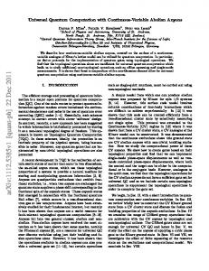
x+

BS

xt

x− XLO θ Figure 2.3: Schematic of an ideal homodyne detection. The quantum target mode (t) is combined with the local oscillator (LO) at a balanced beam splitter (BS). The phase θ of the local oscilator determines the measured quadrature. output modes of the beam splitter read √ x ˆ+ = (ˆ xt + XLO )/ 2, √ pˆ+ = pˆt / 2, √ x ˆ− = (ˆ xt − XLO )/ 2, √ pˆ− = pˆt / 2.

(2.98)

Second, the intensities of these two modes are measured using two photodiodes I± ∝ x ˆ2± + pˆ2±

2 ∝x ˆ2t + XLO + pˆ2t ± 2XLO x ˆt ,

(2.99)

and the two photocurrents are subtracted and amplified with a low noise amplifier. On can easily check that the difference gives an estimation of the measured quadrature I+ − I− ∝ XLO x ˆt .

(2.100)

In order to measure the conjugate quadrature pˆt of the target mode, one simply needs to apply a π/2 phase shift to the local oscillator. In full generality, one can measure a quadrature x ˆθ = cos θˆ xt + sin θ pˆt by shifting the phase of the local oscillator by θ, using for example a piezoelectric transducer (PZT). Although technically challenging, the efficiency of a good homodyne detection scheme can easily reach 90% [57, 66]. 32

2.3. Information Theory

2.3

Information Theory

Finally, one cannot be called a quantum information scientist without basic knowledge of information theory. As mentionned in the introduction, information theory is a mathematical theory developed by Claude Shannon in 1948 to address the problem of the transmission of information over noisy channels. The most fundamental results of the theory are known as Shannon’s source coding theorem and Shannon’s channel coding theorem. The first of these theorems states that, on average, the number of bits needed to represent the result of an uncertain event is given by a quantity called the entropy, while the second guarantees that reliable communication is possible over noisy channels provided that the rate of communication is below a certain threshold called the channel capacity. Remarkably, the concepts introduced by Shannon for the manipulation of classical objects can be adapted to the manipulation of quantum states, which gives rise to the theory of quantum information and communication. Quantities such as the entropy or the capacity have their quantum counterpart known as the von Neumann entropy and the quantum channel capacity respectively. The following section will introduce these basic notions, emphasizing on the parallel between the classical versus the quantum version. Let us mention that most of these quantities will not be used directly in the following chapters, but underly the concepts and challenges of quantum information science as a whole.

2.3.1

Classical Information Theory

Suppose that a source emits a sequence of random variables X1 , X2 , . . . whose values belong to a finite alphabet A = {0, 1, . . . , d}. If the variables are independent and identically distributed according to the probability distribution p(x) = P r{X = x}, x ∈ A, the entropy of the source is defined as X H(X) = − p(x) log p(x) , (2.101) x∈A

where the logarithm is taken in base 2. The entropy gives a useful measure of the uncertainty one has about X before learning its value. Interestingly, it can also be interpreted as the amount of information one gains by learning the value of X. Similarly, one can define the joint entropy H(X, Y ) of a pair of discrete variables (X, Y ) which take values in A1 = {0, 1, . . . , d1 } and A2 = {0, 1, . . . , d2 }, namely X X p(x, y) log p(x, y), (2.102) H(X, Y ) = − x∈A1 y∈A2

33

CHAPTER 2. All you Need to Know About... where p(x, y) = P r{X = x, Y = y}, x ∈ A1 , y ∈ A2 , is their joint probability distribution. Sometimes, the knowledge of the value taken by the variable X provides some information about the possible values of Y and reduces the uncertainty on Y . The average uncertainty we have about Y when X is known is quantified by the conditional entropy H(Y |X) =

X

x∈A1

=−

p(x)H(Y |X = x)

X X

p(x, y) log p(y|x).

(2.103)

x∈A1 y∈A2

Another useful quantity is the relative entropy which quantifies the distance between the two probability distributions p(x) and q(x) on the alphabet A D(p k q) =

X

p(x) log

x∈A

p(x) . q(x)

(2.104)

Finally, the possibility for the entropy and the conditional entropy of the random variable Y to have different values, i.e. H(Y ) 6= H(Y |X), suggests that the variable X contains some information about Y . This common information shared by X and Y can be quantified by the difference H(Y ) − H(Y |X) and is known as the mutual information I(X : Y ) = −

X X

p(x, y) log

x∈A1 y∈A2

p(x, y) p(x)p(y)

= D(p(x, y) k p(x)p(y)).

(2.105) (2.106)

The mutual information measures in bits the amount of classical correlations between the variables X and Y . All the quantities introduced in this subsection are closely connected. One can easily verify that they satisfy H(X, Y ) = H(X) + H(Y |X)

(2.107)

= H(Y ) + H(X|Y ),

(2.108)

I(X : Y ) = H(X) − H(X|Y )

(2.109)

= H(Y ) − H(Y |X)

= H(X) + H(Y ) − H(X, Y ), as graphically illustrated in the Venn diagram of Fig.2.4. 34

(2.110) (2.111)

2.3. Information Theory

H(X)

H(Y)

H(X|Y)

I(X:Y) H(Y|X)

H(X,Y) Figure 2.4: Graphical representation of the various entropies The quantities introduced in this subsection can be easilly used to answer questions related to the transmission of information. For example, the maximal rate at which classical information can be reliably transmitted through a noisy channel T is known as the channel capacity C[T ], and is given by C[T ] = max I(X : Y ) p(x)

(2.112)

where the maximum is taken over all input distributions p(x) for X, for one use of the channel, and Y is the corresponding induced random variable at the output of the channel.

2.3.2

Quantum Information Theory

Suppose now that the source is no longer classical but emits quantum states chosen from an ensemble {|xi} with probability p(x). This can be denoted as {|xi , p(x)}. The state emitted by the source is described by the mixed state X p(x)|xihx|, (2.113) ρ= x

and we can introduce its quantum, or von Neumann, entropy S(ρ) = − Tr(ρ log ρ)

(2.114)

where the logarithm is again taken in base 2. If ρ is diagonal in some eigenbasis {|ii}, then the von Neumann entropy is the Shannon entropy of the eigenvalues λi , i.e. S(ρ) = H(λ). As a consequence, the von Neumann entropy of a pure state is null, while it is maximum for a maximally mixed state. This makes the von Neumann entropy an interesting tool for quantum information theory, and for the theory of entanglement in particular. 35

CHAPTER 2. All you Need to Know About... As an example, consider a bipartite pure state ρAB . If ρAB is maximally entangled, then the reduced state ρA = TrB ρAB is maximally mixed and S(ρA ) is maximum. If ρAB is a product state, however, ρA is a pure state and S(ρA ) = 0. As previously mentionned, the entanglement of a bipartite pure state is completely characterized by the von Neumann entropy of any one of its reduced state. Naturally, for a bipartite quantum system with density matrix ρAB , one can also define the joint entropy S(A, B) S(ρAB ) = − Tr(ρAB log ρAB ),

(2.115)

which enables the definition of the conditional entropy S(A|B) S(A|B) = S(A, B) − S(B).

(2.116)

In contrary to the classical case, the conditional entropy can be negative [22]. This indicates the presence of entanglement as for systems with S(A|B) < 0, the uncertainty about the whole system is less than the uncertainty of one of its constituents. In analogy with Eq. (2.111), the definition of the joint entropy provides a definition of the quantum mutual information [22] S(A : B) = S(A) + S(B) − S(A, B) ,

(2.117)

and we can also introduce the relative entropy D(ρ k σ) = Tr(ρ log ρ) − Tr(ρ log σ),

(2.118)

which provides a useful measure of the distance between the two quantum states ρ and σ. To conclude this section, we note that there exists various quantum capacities, depending on the information one tries to maximise and the ressources and protocols allowed for. For example, the classical information capacity C[T ] of a channel T is the asymptotically achievable number of classical bits that can be reliably transmitted per use of the quantum channel. One can also define the quantum capacity Q[T ], i.e., the number of qubits that can be reliably transmitted through the channel, or the entanglement-assisted classical and quantum capacities CE [T ] and QE [T ], i.e., the rate at which bits or qubits can be transmitted when an infinite amount of entanglement is shared between the sender and receiver [20].

36

3 Testing Quantum Nonlocality 3.1

Introduction

One of the principal features of quantum mechanics is the impossibility to know simultaneously the value of certain physical quantities with unlimited precision. This limitation does not result from our inability to measure these properties properly, because of the current state of technology for example, but is a consequence of the laws of quantum mechanics themselves. As demonstrated in Sec. 2.1.2, when two quantities are described by noncommuting observables, the perfect knowledge of one precludes the perfect knowledge of the other. Many physicists of the early days of quantum mechanics were greatly puzzled by such a counterintuitive aspect of the theory. Einstein, in particular, considered this as a witness of the incompleteness of the theory. In 1935, together with Podolski and Rosen, he advocated his point of view in a seminal paper entitled “Can Quantum Mechanical Description of Physical Reality Be Considered Complete?” [34]. Their argument, sometimes referred as the EPR paradox, was the following. In every complete theory, there should be a variable corresponding to an element of reality (a physical quantity that is possible to predict with certainty without disturbing the system). As mentionned above, quantum mechanics precludes the joint knowledge of two non-commuting observables such as the position and momentum of a particle. Hence, either the description of reality given by quantum theory is incomplete, or these two non-commuting observables cannot 37

CHAPTER 3. Testing Quantum Nonlocality have simultaneous reality. Considering a special bipartite entangled state known has an EPR pair (equivalent to the maximally entangled two-mode squeezed vacuum of Sec. 2.2.5), and the predictions one can make about the second system of this state based on the measurement of the first, they proved that assuming quantum theory to be complete, i.e., rejecting the first proposition, one could nevertheless assign elements of reality to both non-commuting observables, i.e., one must also reject the second proposition. Their conclusion is thus that one’s only choice is to accept the first proposition, and accept that the description of reality given by quantum theory is not complete. To solve the apparent incompleteness of quantum theory, Einstein, Podolski and Rosen introduced the idea of local hidden variables. Their interpretation of quantum mechanics, known as Local Realism or the Local Hidden Variable (LHV) model of quantum mechanics, assumes the existence of variables corresponding to all elements of reality, even if some of these variables are inaccessible to measurement. Interestingly, by reintroducing some classical intuition into the description of physical reality, they provided an explanation to the counterintuitive aspects of quantum mechanics such as entanglement and the probabilistic nature of the theory. For many years, depending on their philosophical background or personal beliefs, physicists around the globe argued about the Local Realistic Vs. Quantum Mechanical description of nature. In 1964, this debate and the EPR argument gained a renewed attention due to the work of John Bell. Assuming local realism to be true, Bell derived his now famous inequality which must be satisfied within the framework of any local realistic theory [7]. Interestingly, this inequality is a relation between conditional probabilities and therefore has a priori nothing to do with quantum mechanics. However, Bell predicted a violation of his inequality by considering the probabilities resulting from local measurements on a maximally entangled state. By doing so, he strikingly refuted the possibility to explain quantum mechanics in terms of a local hidden variable model. But the real merit of his work lied somewhere else. After 30 years of philosophical debate, Bell provided a definitive argument in favor of the nonlocal interpretation of quantum mechanics which could be tested in a laboratory. Ironically, Bell’s inequality was called ”the most profound discovery of science“ [94] although it is not obeyed by the experimental facts. Since 1972 and the first experimental violation of a Bell inequality [42], a great variety of Bell tests have been performed based on various quantum systems. In every experiment, a local realistic description of the experimental results is incompatible with the actual observations. Unfortunately, regardless of the success of these experiments, the local description of nature favored by Einstein has not yet been ruled out completely as all the experiments performed to date suffer from so-called loopholes. These conceptual loopholes, exploiting experimental limitations, force us to rely on supple38

3.2. Bell Tests and Related Loopholes mentary assumptions in order to reject local realism, thereby weakening the strength of Bell’s argument. The emergence of quantum information science, and the related discovery that entanglement and nonlocal correlations could be useful ressources [9, 31], naturally triggered the quest for a Bell test free of loopholes. Since Artur Ekert’s “Quantum Cryptography Based on Bell’s Theorem“ [31], rejecting local realism and understanding the nonlocal nature of physical reality has left the area of fundamental questions for theoretical physicists, to become an essential ingredient for the development of future technologies and applications. However, the lack of a true loophole free Bell test strongly questions the operational use of Bell inequalities in quantum information. If a set of experimental data violates a Bell inequality, can one really conclude that the state under measurement is non local when the detectors are inefficient? In this chapter, we will contribute to this fascinating quest by considering for the first time m-partite Bell inequalities based on quadrature measurements of the electromagnetic field. Due to the high performances of homodyne detection, such systems are known to possibly close two of the main loopholes simultaneously. In particular, we will prove that it is always possible to maximally violate the m-partite Mermin-Klyshko inequality based on such system, thereby opening a new road towards an experimental test of local realism that could tolerate the inevitable experimental imperfections.

3.2 3.2.1

Bell Tests and Related Loopholes The CHSH inequality

Let us first introduce an inequality which is, in its spirit, similar to the one initially derived by Bell. There exists infinitely many Bell inequalities, but the well-known CHSH inequality introduced by John Clauser, Michael Horne, Abner Shimony and Richard Holt in 1969 [24] is certainly the most intuitive one. To fix the rules of the game, consider the following experiment. Suppose that Alice and Bob, who are spatially separated, receive a box from their friend Charles. They can perform measurements on their box, and each must independently choose between two possible measurements, either A1 or A2 for Alice, and B1 or B2 for Bob. These measurements have only two possible outcomes ±1, which are denoted by a1 or a2 , and b1 or b2 respectively. Now assume, as Bell did, that the boxes obey to the local realism of Einstein, Podolski and Rosen. Realism means that the properties measured by Alice and Bob have definite values a1 , a2 , b1 and b2 which exist independently of the act of observation. Locality, on the other hand, imposes that Alice’s choice of measurement and outcome does not influence the result 39

CHAPTER 3. Testing Quantum Nonlocality of Bob’s measurement (and vice versa). It follows that the measurement results satisfy a1 (b1 + b2 ) + a2 (b1 − b2 ) = ±2

(3.1)

This is so because either b1 + b2 = 0 and b1 − b2 = ±2 or b1 − b2 = 0 and b1 + b2 = ±2. However, it is important to note that this identity corresponds to four different tests that cannot be performed simultaneously, some of them are counterfactual [84]. Nevertheless, the meaning of the identity is guaranteed by the assumptions of realism and locality; realism ensures that all the quantities involved in (3.1) have a simultaneous meaning, while locality is necessary to obtain the value of ±2 on the right hand side. If we now perform many runs of this experiment, we can compute the value of (3.1) on average, which easily leads to the well-known CHSH inequality |ha1 b1 i + ha1 b2 i + ha2 b1 i − ha2 b2 i| ≤ 2

(3.2)

where hai bj i = P (ai = bj ) − P (ai 6= bj ) is the average value, or the correlation coefficient, for the measurement of Ai by Alice and Bj by Bob. Recall that (3.2) was derived only assuming locality and realism, i.e., it has to be satisfied by any local realistic theory. Now suppose that the boxes given to Alice and Bob contain a quantum system. In particular, suppose that the boxes contain each one half of the maximally entangled singlet state 1 |Ψ− i = √ (|0iA |1iB − |1iA |0iB ) 2

(3.3)

and that the possible measurement settings available to Alice and Bob correspond to A1 = σx A2 = σz 1 B1 = √ (σx + σz ) 2 1 B2 = √ (σx − σz ) 2 where σx and σz are the standard Pauli operators [78], and |0i and |1i are the eigenvectors of σz . Quantum mechanics does not allow the simultaneous consideration of the results of measurements of non-commuting observables, hence for quantum mechanical boxes the identity (3.1) is meaningless. However, quantum mechanics allows the calculation of average values. In particular, we can calculate the average value of the Bell operator S = A1 ⊗ B1 + A1 ⊗ B2 + A2 ⊗ B1 − A2 ⊗ B2 40

(3.4)

3.2. Bell Tests and Related Loopholes

a1 (a2)

b1 (b2)

Alice

Bob

A1 (A2)

B1 (B2)

Figure 3.1: Schematic of a Bell test with two parties and two settings for a given quantum state. When the boxes are described by the state |Ψ− i, a few lines of calculation show that the Bell factor B = |hSi| = |hA1 ⊗ B1 i + hA1 ⊗ B2 i + hA2 ⊗ B1 i − hA2 ⊗ B2 i| √ (3.5) =2 2 which exceeds the maximum of 2 allowed by Eq. (3.2). Remarkably, quantum mechanics predicts a violation of the CHSH inequality of around 41%.

3.2.2

Detector Efficiency and Locality Loophole

One should not forget that quantum mechanics is a theory about experimental facts. Ultimately, rejecting local realism will have to be done based on experimental data gathered in a laboratory. But experiments are never perfect. They suffer from errors, imperfections, and technological limitations. In order to successfully show that the results of an experiment cannot be explained by a local hidden variable theory, one has to include all these experimental parameters in the local realistic model of the experiment. Following Freedman and Clauser remarkable experiment in 1972 [42], many Bell tests confirmed the violation of Bell inequalities by quantum mechanics (see e.g. Aspect’s experiments [3, 4, 5]). All these early attempts were based on the polarization degree of freedom of photons as it was, for many years, the only known way to generate the necessary entanglement between two distant location. Unfortunately, detecting a photon is a difficult task, and photon detectors are known to suffer from low efficiencies (today typically around 10% [63]). As first noted in [83], this low efficiency can be exploited to explain the observed violation of a Bell inequality with a local hidden variable model. To avoid this problem, one has to make an additional assumption; namely that the registered pairs of photons form a fair sample 41

CHAPTER 3. Testing Quantum Nonlocality of the emitted pairs. This is the so-called detector efficiency loophole. From a logical point of view, none of the experiments based on photon pairs have successfully succeeded in ruling out local realism. This loophole was finally closed a few years ago [90, 73], using an entangled pair of trapped ions. The benefit of this novel approach is the high efficiency of the ion state detection. Unfortunately again, entangling ions over large distances is extremely challenging. In the experiments mentioned above, the ions were maintained only several micrometers and one meter apart respectively. So close that the measurement events could not be considered truly space-like separated as required by a local realistic model. This is known as the locality loophole. So far, no experimental test has succeeded in closing both loopholes simultaneously.

3.3 3.3.1

Bell Tests and Continuous Variables Bell Tests Based on Quadrature Measurements

There is a large variety of quantum systems for which a test of local realism may be envisaged. However, the quest for a loophole free Bell test has recently focused the research towards experiments involving propagating light modes measured with homodyne detectors [76, 102, 44, 45, 77]. The advantage of this approach is twofold. On the one hand, light modes can easily be sent to space-like separated detectors thereby avoiding the locality loophole. On the other hand, the current technology of homodyne detectors achieves a degree of detection efficiency high enough to close the detection efficiency loophole. Unfortunately, the use of continuous variables with homodyne detection also implies drawbacks whose resolution is challenging. The main issue is that the homodyne measurement of a state with a positive Wigner function can always be described with a local hidden variable model. Thus, in order to avoid a local hidden variable description of the measured correlations, one has to perform the test with a state endowed with a non-positive Wigner function. In particular, the easily generated two-mode squeezed state of the EPR argument cannot be directly employed as its positive Wigner function provides a local realistic model explaining all correlations between quadrature measurements. Several theoretical work have recently demonstrated the possibility to violate a Bell inequality by measuring the quadratures of specifically tailored entangled non-Gaussian states of light. These tests generally involve the following scenario. Two parties perform spacelike separated homodyne measurements by randomly choosing between two settings, thus measuring two quadratures of the incoming electromagnetic fields. The collected data, which are distributed in a (approximately) continuous range, are discretized in a procedure called the binning process, and the violation of the CHSH 42

3.3. Bell Tests and Continuous Variables inequality is then tested [24]. Interestingly, these tests can be divided in two categories depending on the magnitude of the predicted violation and the feasibility of the envisioned experimental setup. Large violation: In [76], Munro identified what ideal correlated photon number state is required to maximally violate the CHSH inequality when homodyne detection is used in combination with a simple binning based on the sign of the measured quadrature. More specifically, he considers the state |Ψi =

∞ X

n=0

cn |ni |ni ,

(3.6)

where |ni is a Fock state, and optimizes over both the quadrature angles of the measurement and the coefficients cn of the state. This leads to a maximal violation of B ≈ 2.076 1 . Furthermore, it was later shown √ in [102] that one can even reach the maximal possible value of B = 2 2 by measuring conjugated quadratures of states of the form 1 |Ψi = √ (|f i |f i + eiθ |gi |gi) , 2

(3.7)

where f and g are appropriately chosen wave functions, and a special binning based on the roots of the f anf g functions is applied. This will be explained and further extended in Sec. 3.4.2. Unfortunately, the experimental generation of these two types of states is extremely challenging, clearly out of reach of present day technology. Experimentally feasible: Along a different line of thought, two recent proposals [44, 77] predicted the violation of local realism by considering a state closer to an experimental realization. The state in question is a twomode squeezed vacuum to which photons have been subtracted. Given the recent sucessful photon subtraction experiments [81, 82], this state is clearly within the reach of present technology. However, the achievable violation with such a photon subtracted squeezed vacuum is so low, around 2, 2%, that the inevitable experimental imperfections have so far been sufficient to discourage experimentalists from carrying out the experiment.

3.3.2

Multimode Nonlocality

The proposals for loophole free Bell tests relying on homodyne detection have, so far, considered only two parties and the CHSH inequality. This is 1

If we restrict to positive cn ’s as will be seen in Sec. 3.4.1

43

CHAPTER 3. Testing Quantum Nonlocality the simplest scenario, both conceptually and experimentally. However, there exist multipartite Bell inequalities testing the local realism of m-partite entangled states. One such inequality is the Mermin-Klyshko (MK) inequality [74, 67], a generalization to m parties of the CHSH inequality. Interestingly, quantum mechanics predicts an exponentially increasing violation of this inequality with the number of parties involved, i.e., for m parties the maximal violation is [49] Bm = 2(m+1)/2

(3.8)

while local realism remains bounded by 2. We note that multipartite settings with continuous variable states have already been considered, but relying on measurement strategies other than homodyne detection. In Ref. [97] for example, a test based on the measurement of the light field parity is envisaged. It is found that the violation does not increase exponentially, as one would have hoped, but this could be due to the fact that no optimization over the possible measurement settings was performed [37]. In Ref. [23] instead, a maximal violation of the Mermin-Klyshko inequality is found for continuous variable states, considering the measurement of a special class of operators which can be seen as the continuous-variable analogue of the spin operator. However, both of these approaches deal with non-Gaussian measurements described by a non-positive Wigner function. Such measurements are far from the reach of current detection technology. We note also that very recently, a new approach was introduced which does not rely on the use of inequalities for discrete outcomes, thus avoiding the need of a binning procedure [19]. The authors found that the violation of the local realistic bound is exponential in the number of parties involved, but a possible experimental implementation is still very challenging as it would require at least ten space-like separated homodyne measurements. It is then unclear if such a novel approach can give advantages, from a practical perspective, over the non-locality tests involving binning strategies presented in the next section.

3.4

Multimode Nonlocality using Homodyne Detection

Given this previous work, we ask the following question: Is it possible to have an exponential increase of the violation of local realism in a test involving quadrature measurements of m modes and considering Mermin-Klyshko inequalities? 44

3.4. Multimode Nonlocality using Homodyne Detection

3.4.1

Correlated Photon Number states

Before we start, let us recall the general form of the Mermin-Klyshko Bell inequalities. As for the CHSH inequality, we consider two dichotomic observables Ot and Ot′ for each party t. The Mermin-Klyshko inequalities are then based on the following recursive definition of the Bell operator: Bt ≡

1 1 ′ Ot + Ot′ ⊗ Bt−1 + Ot − Ot′ ⊗ Bt−1 , 2 2

(3.9)

where B1 = 2O1 , B1′ = 2O1′ , and Bt′ denotes the same expression as Bt but with all the Ot ’s and Ot′ ’s exchanged [49]. The Mermin-Klyshko inequality for m parties then reads Bm ≡ |hBm i| ≤ 2 .

(3.10)

Let us now consider a generic photon number correlated state of m bosonic modes ∞ X cn |ni1 |ni2 ... |nim , (3.11) |Ψi = n=0

P 2 with n |cn | = 1. This is the generalization to m modes of the state considered in Ref. [76]. There, two quadratures of the electromagnetic field X(θt ) and X(θt′ ) (corresponding to two angles θ and θ ′ ) are chosen as the two observable Ot and Ot′ to be measured. Recall that the quadrature X(θt ) of each mode t can be measured via homodyne detection. If we introduce the notation Xt (Xt′ ) for the quadrature X(θt ) (X(θt′ )), and xt (x′t ) for the outcome of its measurement, the joint probability to obtain the results x1 , ..., xm by measuring the quadratures X1 , ..., Xm is given by P(x1 , ..., xm ) = |1 hx1 | ... m hxm | Ψi|2 ∞ m X Y eiφ(n−s) 2 ∗ cn cs e−xt Hn (xt )Hs (xt ) , = × n+s m/2 (π2 n!s!) n,s=0 t=1 where φ = θ1 + ... + θm , Ht (x) is the t-th degree Hermite polynomial, |xt i are the eigenvectors of the quadrature operator Xt , and we have used the coordinate representation of the Fock states Eq. 2.57. Consider now a simple binning strategy, the so called sign binning: when the result of a quadrature measurement falls in the domain R+ 0 , we associate to it the value +1, when it is in R− , we give it the value −1. Based on this binning, we can calculate the probability P+1,...,+1 that a “+1” result is 45

CHAPTER 3. Testing Quantum Nonlocality observed in all the measuring sites: Z ∞ Z ∞ dxm P(x1 , ..., xm ) dx1 ... P+1,...,+1 = 0

0

∞ X

=

m

cn c∗s

n,s=0

Y eiφ(n−s) × n+s m/2 (π2 n!s!) t=1

Z

∞

2

dxt e−xt Hn (xt )Hs (xt ) .

0

(3.12)

The integrals above can be evaluated recalling the following properties of Hermite polynomials for n 6= s, Z ∞ π2n+s 2 [F (n, s) − F (s, n)] , (3.13) dxt e−xt Hn (xt )Hs (xt ) = n−s 0 where we defined F (n, s) as F (n, s)−1 = Γ

1 1 1 − n Γ − s , 2 2 2

with Γ being the gamma function. For n = s one has instead Z ∞ √ 2 dxt e−xt Hn2 (xt ) = 2n−1 n! π .

(3.14)

(3.15)

0

Defining the functions X G(φ, m) = 2Re(cn c∗s )gn,s (φ, m) , n>s

gn,s (φ, m) =

π2n+s n!s!

m/2

F (n, s) − F (s, n) n−s

m

× cos[φ(n − s)] ,

(3.16)

one obtains P+1,...,+1 =

1 + G(φ, m) . 2m

(3.17)

The other probabilities can be obtained in a similar way. Let us define the multi-index d = (d1 , ..., dm ), with dt = ±1 denoting the measurement result obtained for mode t after the binning. Then, the joint probability for a generic collection d of measurement results will be indicated by Pd and it can be obtained as above by recalling that an Hermite polynomial of even (odd) degree is an even (odd) function. An explicit formula for the generic probability Pd can then be calculated: Pd = where σ(d) =

Qm

1 + σ(d)G(φ, m) , 2m

t=1 dt .

46

(3.18)

3.4. Multimode Nonlocality using Homodyne Detection Now we are in the position to calculate the generic correlation function between the measurement results E(φ, m). Notice that the correlation depends only on the sum of the angles φ. By definition we have that X E(φ, m) = σ(d)Pd , (3.19) d

where the sum goes over all the possible collection of measurement results. Since the number of possible measurement results for which σ(d) = 1 is equal to that for which σ(d) = −1 one finally has, by substituting Eq. (3.18) into Eq. (3.19), that E(φ, m) = 2m G(φ, m) .

(3.20)

Let us show that we can reach an exponential violation with a simple analytical manageable example. For the simple case of three parties (m = 3), the Mermin-Klyshko inequality then reads B3 ≡ |hB3 i| ≤ 2, with B3 = O1 ⊗ O2 ⊗ O3′ + O1 ⊗ O2′ ⊗ O3 + O1′ ⊗ O2 ⊗ O3 − O1′ ⊗ O2′ ⊗ O3′ . (3.21) Considering a tripartite GHZ state [55], 1 |GHZ3 i = √ (|000i + |111i) , 2

(3.22)

we have c0 = c1 = 2−1/2 and cr≥2 = 0, so that G(φ, 3) = g1,0 (φ, 3) = (2π)−3/2 cos(φ) and Eq. (3.20) becomes 3/2 2 E(φ, 3) = 2 G(φ, 3) = cos(φ). π 3

(3.23)

The GHZ-like angles (θ1 = 0, θ2 = π/6, θ3 = 2π/6, and θi′ = θi + π/2), give the maximum violation of the inequality, namely B3 = |3 E(π, 3) − E(0, 3)| 3/2 2 =4 π ≃ 2.032 .

(3.24)

Now, consider the multipartite generalization of the GHZ state 1 |GHZm i = √ (|0...0i + |1...1i) , 2 47

(3.25)

CHAPTER 3. Testing Quantum Nonlocality

Figure 3.2: Coefficients cn for the optimal state |Ψi in the case of m = 3, d = 20 (with GHZ-like measurement angles). The Bell factor is B3 ≃ 2.204. and Eq. (3.20) becomes m/2 2 E(φ, m) = cos φ . π

(3.26)

The dependence on the angle φ of the above correlations is the same as the one appearing in a standard spin-like test for a multipartite GHZ state, namely E(φ) = cos(φ). In that case, it is known that the choice of GHZ-like angles θk = (−1)m+1 π(k − 1)/(2m) θk′

= θk + π/2,

(3.27) (3.28)

gives the highest value of the Bell factor, namely 2(m+1)/2 [49]. Therefore, using the same angles, the corresponding Bell factor reads Bm =

√

2

m/2 4 , π

(3.29)

giving rise to an exponential violation of local realism. Apart from this simple analytical example, one can use a numerical approach to show the exponential violation of local realism as the formula (3.20) is easily amenable to perform numerical calculations for a fixed number of parties m. In order to find the state |Ψi (coefficients cn ’s) that maximally violates the Mermin-Klyshko inequality, one has to evaluate the corresponding Bell factor Bm for a given configuration of measuring angles. 48

3.4. Multimode Nonlocality using Homodyne Detection

Figure 3.3: Coefficients cn for the optimal state |Ψi in the case of m = 2, d = 30. The Bell factor is B2 ≃ 2.1. The Bell factors are expressed in general by a linear combination of correlation functions given each by Eq. (3.20), with the prescription given in Eq. (3.9). Let us search the state which maximizes the violation of the MerminKlyshko inequality for the particular GHZ-like choice of angles. For three modes (m = 3), defining the (infinite dimensional) real symmetric matrix B3 as [B3 ]n,s = 23 (3gn,s (π, 3) − gn,s (0, 3)) , (3.30) where the diagonal elements are set to zero, we note that the Bell factor can be re-expressed as B3 = C † B3 C, where the elements of the vector C are given by the coefficients of the input state, i.e. [C]n = cn . Consequently, the maximal violation of the Mermin-Klyshko inequality is simply given by the maximal eigenvalue of the matrix B3 , while the optimal input state is determined by its corresponding eigenvector. In order to perform a numerical analysis, one has to truncate the Hilbert space dimension of |Ψi to some arbitrary d. For example, for d = 2 the optimal choice turns out to be the GHZ state (3.22), giving a violation of B3 = 2.032. By increasing the dimension d, the asymptotic violation is given by B3 ≃ 2.205. In Fig. 3.2, we show the coefficients cn for the optimal state |Ψi in the case d = 20, for which the Bell factor is B3 ≃ 2.204. The same procedure can be applied for any number of parties. In the case of two parties (m = 2), one recovers the results given by Munro in Ref. [76] provided that the constraint cn > 0 is taken into account, namely B2 ≃ 2.076. Interestingly, a higher violation can be achieved if we consider negative coefficients for |Ψi. As an example, we report in Fig. 3.3 the coefficients cn for the optimal state in the case d = 30, for which the Bell factor 49

CHAPTER 3. Testing Quantum Nonlocality rises up to B2 ≃ 2.100 (recall that the Bell factor can be written in this case as B2 = 3E(φ) − E(3φ), where we have chosen φ = π/4, as in [76]).

3.4.2

Maximal Violation

Let us now see whether we can find a class of states and a binning strategy that allows for a maximal violation of the Mermin-Klyshko inequality for any number of parties m. Recall that quantum mechanics is bounded by Eq. (3.8). Inspired by the results of Ref. [102], we introduce the state 1 |Ψi = √ (|f i⊗m + eiθ |gi⊗m ) , 2

(3.31)

where f is a real and even function of some quadrature x, while g is real and odd. The two functions are orthogonal and normalized to unity. Note that because f (x) is real and even, it has a real and even Fourier transform ˜ ˜ f˜(p), while g(x) has an imaginary Fourier transform ih(p), with h(p) real and odd. Suppose that each party t chooses to measure one of two conjugated quadrature via homodyne detection, either X(0) = X or X(π/2) = P , and obtains a continuous variable xt or pt depending on his choice of measurement setting. When the k first parties measure the X quadrature, while the remaining m − k measure the conjugate quadrature P , the joint probability that they obtain the results x1 , ..., xk , pk+1 , ..., pm is given by P(x1 , ..., xk , pk+1 , ..., pm ) = |hx1 |...hxk |hpk+1 |...hpm |Ψi|2 1 = f 2 (x1 )...f 2 (xk )f˜2 (pk+1 )...f˜2 (pm ) 2 ˜ 2 (pk+1 )...h ˜ 2 (pm ) + g2 (x1 )...g2 (xk )h π + 2 cos(θ + (m − k) ) × f (x1 )g(x1 )...f (xk )g(xk ) 2 ˜ ˜ ˜ ˜ m) . × f (pk+1 )h(pk+1 )...f (pm )h(p (3.32) To exploit the parity properties of f ang g, we introduce the root binning defined in Ref. [102]. This binning depends on the roots of the known functions f and g. If party t measures the X quadrature, the result will be interpreted as a “+1” if the measured value xt lies in the interval where f (xt ) and g(xt ) have the same sign, and “−1” if their signs are opposite, i.e., we consider the following domains Dx+ = {x ∈ R|f (x)g(x) ≥ 0}

Dx− = {x ∈ R|f (x)g(x) < 0} .

(3.33)

We can similarly define the domains Dp+ and Dp− associated to the measurement of the quadrature P . For the choice of measurement settings defined 50

3.4. Multimode Nonlocality using Homodyne Detection above, we can thus calculate 2m probabilities Pd corresponding to the observation of a given collection d of binary results. For example, the probability P+1,...,+1 that each party observes a “+1” result reads P+1,...,+1 =

Z

Dx+

dx1 ...

Z

Dx+

dxk

Z

Dp+

dpk+1 ...

Z

Dp+

× P(x1 , ..., xk , pk+1 , ..., pm ) .

dpm (3.34)

We are now in the position to calculate the correlation function ˜ are even and E(X1 , ..., Xk , Pk+1 , ..., Pm ). Note that since f and g (f˜ and h) 2 2 2 2 ˜ ˜ odd respectively, f and g (f and h ) are even functions. Hence the first two terms of the right hand side of (3.32) are even functions also, and their contribution to the correlation function will vanish. We thus obtain the remarkably simple expression h πi , (3.35) E(X1 , ..., Xk , Pk+1 , ..., Pm ) = V k W m−k cos θ + (m − k) 2 where V = W =

Z

∞

Z−∞ ∞ −∞

|f (x)g(x)|dx

(3.36)

˜ |f˜(p)h(p)|dp .

(3.37)

Interestingly, the correlation function (3.35) only depends on the number of sites where X and P are measured. One can easily check that all correlation functions corresponding to k measurements of the X quadrature and m − k measurements of the P quadrature are equal. We will denote them E(k, m− k) to emphasize this property. Let us illustrate the power of this compact notation with an example. For m = 3, the Bell factor reads B3 =|E(X1 , X2 , P3 ) + E(P1 , X2 , X3 ) + E(X1 , P2 , X3 ) − E(P1 , P2 , P3 )| =|3E(2, 1) − E(0, 3)| π π =|3V 2 W cos(θ + ) − W 3 cos(θ + 3 )| . 2 2

(3.38)

We see that the maximal violation, i.e. B3max = 4, can be reached with a state |Ψi such that sin(θ) = ±1 and V = W = 1. Although such a state is quite unrealistic, one can define a family of physical states that approximates it arbitrarily well. The corresponding f ang g functions are trains of gaussians, and V, W → 1 as the number of peaks goes to infinity. We refer the reader to Ref. [102] for their exact analytical expression.

51

CHAPTER 3. Testing Quantum Nonlocality Let us now try to generalize this result for an arbitrary m. First note that the Bell factor (3.10) can be written as 1 ′ ′ i − hPm Bm−1 i| , (3.39) Bm = |hXm Bm−1 i + hPm Bm−1 i + hXm Bm−1 2 with B1 = 2X1 and B1′ = 2P1 . In order to benefit from our compact ′ notation, we explicitly develop the expectation values of Bm−1 and Bm−1 in terms of correlation functions hBm−1 i = ′ hBm−1 i=

m−1 X

k=0 m−1 X k=0

αk E(k, m − 1 − k) αk E(m − 1 − k, k)

(3.40)

where the αk ’s are some known coefficients. When m − 1 = 3 for example, we have α1 = 3, α3 = −1, and α0 = α2 = 0. As the correlation functions only depend on the number of X and P measurements, the average values of the four operators of (3.39) can be easily calculated from hBm−1 i and ′ hBm−1 i. Suppose Bm−1 has a term proportional to the X1 ...Xk Pk+1 ...Pm−1 operator, which leads to the correlation function E(k, m − 1 − k). The operator Xm Bm−1 will thus have a term proportional to Xm X1 ...Xk Pk+1 ...Pm−1 leading to the correlation function E(k + 1, m − 1 − k), i.e. at the level of correlation functions we only need to replace k by k + 1 as the X quadrature is measured at one additional site. A similar argument for the expectation ′ ′ leads to and Pm Bm−1 values of Pm Bm−1 , Xm Bm−1 m−1

1 X αk E(k + 1, m − 1 − k) + E(k, m − k) Bm = | 2 k=0 +E(m − k, k) − E(m − k − 1, k + 1) |

(3.41)

To maximize this expression, we note that for two and three parties the maximum violation is reached for a state with V = W = 1. It is thus reasonable to assume that this property remains true for an arbitrary m. Recall that we know how to choose f and g such as to reach these values. When V = W = 1, we have h πi , (3.42) E(k, m − k) = cos θ + (m − k) 2 and (3.40) becomes hBm−1 i = ′ hBm−1 i=

m−1 X

k=0 m−1 X k=0

h πi αk cos θ + (m − 1 − k) 2

(3.43)

h πi αk cos θ + k 2

(3.44)

52

3.4. Multimode Nonlocality using Homodyne Detection Introducing Eq. (3.42) in Eq. (3.41), combined with some well known trigonometric formulas, the Bell factor simplifies to m−1

Bm

h X π πi π αk cos (m − 2k) | . (3.45) = | cos(θ + m ) + sin(θ + m )| × | 4 4 4 k=0

Maximizing the violation of local realism boils down to finding the optimal phase θm such that the first factor √ of the right hand side is maximum. This term achieves its maximum of 2 for a value of the phase θm = (1 − m)

π 4

(3.46)

We also note that (m − 2k)

π π = θm−1 + (m − 1 − k) 4 2

(3.47)

hence the maximum value of the Bell factor can be finally written as max Bm

= =

√ √

2| 2

m−1 X

h πi αk cos θm−1 + (m − 1 − k) | 2

k=0 max Bm−1

(3.48) (3.49)

where we have identified the summation of Eq. (3.48) with Eq. (3.43) at the optimal angle θm−1 . Introducing now the √ maximum value obtained in max Ref. [102] for the two party case, B2 = 2 2, we obtain by recursion max Bm = 2(m+1)/2

(3.50)

which is the known maximal bound imposed by quantum mechanics. Remarkably, the state |Ψi defined in (3.31) combined with homodyne detection and a binning strategy called root binning allows for a maximal violation of the MK inequality. This result shows that even if the binning process discretizing the result of the homodyne detection discards some information, it does not prevent to maximally violate tests of local realism based on discrete variables.

3.4.3

Noise Effects

As shown in the previous sections, the search of loophole-free Bell tests could benefit from an increased number of parties involved in the experiment. The signature of this improvement lies in the exponential increase of the Bell factor with the number of parties m. However, what makes a Bell test challenging in practice is not the magnitude of the violation, but rather the inevitable noise associated with any real experiment. In many cases, this noise is sufficient to hide the nonlocal correlations one tries to observe. 53

CHAPTER 3. Testing Quantum Nonlocality When the number of parties involved in a Bell test increases, so does the fragility of the state used in the experiment. The risk is thus to rescale the violation so that no benefit of a larger m is witnessed in practice. One can therefore correctly argue that an increased violation of local realism is only significant if accompanied by a comparable improvement of the robustness to noise of the test. After all, Bell tests have to be verified in a lab, not on paper. In a discrete variable setting, the question of the tolerance to noise of a Bell test is often investigated introducing the noise fraction [68]. The noise fraction quantifies the maximum amount of depolarizing noise one can add to an entangled state and still detect non-local correlations. The depolarizing noise is characterized by the state 1/d, where d is the dimension of the Hilbert space. However, in the continuous variable regime, the Hilbert space under consideration is infinite dimensional and the noise model underlying the noise fraction is irrelevant. Even if we deal with a finite number of photons, such as with the truncated photon number correlated states, the Hilbert space under consideration remains infinite dimensional. Hence the appropriate base is the infinite photon number base and operators proportional to the identity 1 have no physical meaning. To adopt an objective measure of the magnitude of the violation of local realism, one must thus introduce an appropriate CV noise model. The noise we will consider in this section is called probabilistic erasure 2 . Consider the following scenario: with a probability p, the system of a random party is erased, otherwise his state is untouched. This noise acts independently on each site and transforms an initial state |Ψi to m X Trt (|ΨihΨ|) ⊗ |0it h0|} ρ = (1 − p)m |ΨihΨ| + p(1 − p)m−1 { t=1

m

+ ... + p |0i1 h0| ⊗ ... ⊗ |0im h0| .

(3.51)

Probabilistic erasure is known to appear in, e.g. atmospheric transmissions, and has recently been studied in Ref. [104]. This noise will also be considered in Chapter 7. Let us first consider the photon number correlated states of subsection 3.4.1, and concentrate on the second term of Eq. (3.51). Each element of the sum corresponds to the erasures of one of the subsystems, so suppose for example that the state of party m has been erased and replaced by vacuum while distributing |Ψi. The corresponding state shared between the 2

Note that in a real experiment, the most probable sources of noise will be losses and the inefficiency of homodyne detection. Probabilistic erasure is chosen because it can be easily treated analytically.

54

3.5. A Three-Partite Candidate for a Loophole Free Bell Test m parties reads ρ1,m = Trm (|ΨihΨ|) ⊗ |0im h0| ∞ X |cn |2 |ni1 hn| ⊗ ... ⊗ |nim−1 hn| ⊗ |0im h0| . =

(3.52)

n=0

This state is diagonal in the photon number bases, hence the results of all possible measurements are equiprobable, i.e. ∀θ1 , ..., θm , P (x(θ1 ), ..., x(θm )) = cst, and all correlation coefficients vanish. This was to be expected from photon correlated states as their entanglement is truly m-partite; tracing out one subsystem makes the state become separable. Thus, this property also holds for the other noisy terms of (3.51), so that only the erasure-free |ΨihΨ| will contribute to the Bell factor. We obtain Bρ = (1 − p)m Bm

(3.53)

To illustrate this result, consider the m-partite GHZ state (3.25). The noisy Bell factor reads √ 4 (3.54) Bρ = (1 − p)m 2( )m/2 , π hence the maximum probability of erasure pmax such that nonlocal correlations can be detected is √ π 1/2m 2 . (3.55) pmax = 1 − 2 √ This value exponentially tends towards 1 − π/2 as m goes to infinity, and we observe the desired increased robustness to noise as m becomes large. Finally, consider now the states of Section 3.4.2. First note that hf |gi = 0, hence in the {|f i, |gi} bases, these states look like GHZ states. We thus expect their robustness to noise to behave like the photon correlated number states. Indeed, going through the calculation, one finds that for every noisy term of (3.51), and for every choice of measurement setting the probability is an even function of the results. For example, if party m looses its mode, the probability P (x1 , ..., xm ) to obtain x1 , ..., xm given that X1 , ..., Xm is measured is an even function. As a result, none of the noisy terms contribute to the correlation coefficients, and the noisy Bell factor is again given by (3.53) as expected. As a conclusion, with respect to probabilistic erasure, more parties means more robustness.

3.5

A Three-Partite Candidate for a Loophole Free Bell Test

Let us now see how the results of the previous section can be exploited to individuate multipartite states such that, on the one hand, they exhibit a 55

CHAPTER 3. Testing Quantum Nonlocality significantly high violation of local realism and, on the other hand, they may be generated with near future technology. In particular, we will focus on a class of three-party state whose generation involves four so-called optical “Schr¨ odinger-cat” states, that is four single mode superpositions of coherent states [81]. We note that a natural candidate to reach our goal could have been the generalization of the photon-subtracted state discussed in Refs. [44, 77]. However, due to symmetry reasons combined with the use of the sign binning, the generalization to three party (actually to any odd number of parties) of the strategy adopted in Refs. [44, 77] is not effective. In Ref. [102], the authors propose to use a superposition of Gaussians to implement the functions f and g of Eq. (3.31). In particular, in the case of only two Gaussians they considered the family of states defined by f (x) = hx| [c+ (|αi + |−αi)] , g(x) = hx| [c− (|αi − |−αi)] ,

(3.56a) (3.56b)

where 2

c2± = 1/[2(1 ± e−2|α| )].

(3.57)

Given these functions, one can then calculate the corresponding V and W coefficients using Eq. Eq. (3.36). For large amplitudes |α| → ∞, this gives V = 1 and W ≃ 0.64. As noticed in Ref. [102], with two parties no violation is possible, i.e B2 ≃ 1.90. However, as can be seen in Eq. (3.38), considering three parties already enables a violation as large as B3 ≃ 2.23. The corresponding state reads 1 |Ψ3 i = √ c3− (|αi − |−αi)⊗ 3 + c3+ (|αi + |−αi)⊗ 3 , 2

(3.58)

where we have put θ = 0. Since the maximum violation is achieved for large amplitudes, we consider the following simpler state: ′ Ψ = c′ [|α, α, αi + |α, −α, −αi + |−α, α, −αi + |−α, −α, αi] , (3.59) 3

where

2

c′2 = 1/[4(1 + 3e−4|α| )] .

(3.60)

Notice that |Ψ′3 i coincides with |Ψ3 i when |α| → ∞. In order to obtain the Bell factor B3 corresponding to such a state, we calculate the probabilities of the binned outcomes using Eq. (3.56) to define the roots, in combination 56

3.5. A Three-Partite Candidate for a Loophole Free Bell Test 2.4 2.2 2

B3

1.8 1.6 1.4 1.2 1

0.7

0.8

0.9

1

1.1

1.2 |α|

1.3

1.4

1.5

1.6

1.7

Figure 3.4: Bell factor B3 for the state |Ψ′3 i as a function of the amplitude |α|. with Eqs. (3.32) and (3.34). Specifically, we consider the domains Dx± and Dp± inherited by the state |Ψ3 i: Dx+ = {x ∈ R|x ≥ 0} Dx− Dp+ Dp−

(3.61a)

= {x ∈ R|x < 0}

(3.61b)

= {p ∈ R| − cos(pα) sin(pα) < 0} .

(3.61d)

= {p ∈ R| − cos(pα) sin(pα) ≥ 0}

(3.61c)

The Bell coefficient B3 calculated with such a procedure is shown in Fig. 3.4. One can see that for amplitudes as small as |α| ≃ 1.1, the state |Ψ′3 i already gives values above the local bound. We note that in this regime of small amplitudes, |Ψ′3 i = 6 |Ψ3 i and the domains defined in Eqs. (3.61) might be non-optimal. As α is increased, a violation around 10% of the MK inequality is rapidly achieved. Now let us describe how the state |Ψ′3 i may be conditionally generated by using linear optics and superpositions of coherent states (SCS) of the form: |SCSi = c+ (|αi + |−αi). (3.62)

Consider the scheme depicted in Fig. 3.5. Two copies of the state |SCSi in mode a0 and a1 are mixed in a balanced beam splitter. The same action is performed on modes a2 and a3 . Note that mixing two copies of |SCSi on a balanced beam splitter gives √ E √ E E √ E √ |SCSi |SCSi −→ c2+ [ 2α, 0 + 0, 2α + 0, − 2α + − 2α, 0 ] (3.63)

57


Figure 3.5: Schematic of a possible way to conditionally generate the state |Ψ′3 i of Eq. (3.59): (|SCSi) superposition of coherent states [see Eq. (3.62)]; (BS) balanced beam splitter; (D) homodyne detector. Then modes a′1 and a′2 , as well as a′0 and a′3 are respectively mixed by means of two other beam splitters. As a last step mode a′′0 is measured via a homodyne detector. One can easily show that when the measurement outcome −α is obtained, then the conditional state of the remaining modes coincides (approximately) with |Ψ′3 i. To conclude this section, let us note that generating four states |SCSi is experimentally demanding. However, the generation in traveling light modes of such Schr¨ odinger-cat state has been recently reported by many groups (see e.g.[81]). One may thus envisage the possibility to implement the whole scheme described in Fig.3.5 in the near future.

3.6

Conclusion

The developpement of QIS has seen an increasing interest towards the characterization and understanding of nonlocal correlations and entanglement. The main tool to verify the existence of such nonlocal correlations between space-like separated locations is to check that the collected data violate a Bell inequality. Unfortunately, technological limitations and imperfections open so-called loopholes, which have to be closed in order to satisfactorily establish the nonlocal nature of quantum mechanics. To date, no experimental Bell test has succeeded in closing these loopholes simultaneously. Optical continuous variables, combined with the fast and efficient homodyne detection, are an interesting candidate for the experimental implementation of a loophole free Bell test. In theory, they enable to close the detection and locality loophole simultaneously. However, the difficulty to generate non-Gaussian states efficiently makes this approach experimentally challenging, and the proposals closer to an experimental realization predict only a small violation of Bell inequalities, whereas the higher violations involve states whose generation is currently out of experimental reach. In this chapter, we opened a new road in this fascinating quest by in58

3.6. Conclusion vestigating the possibility to increase the number of parties involved in a Bell test based on such quadrature measurements of light modes. Our results show that the violation of the m-partite Mermin-Klyshko inequality grows exponentially with the number of parties involved in the test when one uses photon correlated number states combined with a simple binning strategy. Furthermore, by tailoring the state and the binning procedure appropriately, we have proven the possibility to reach maximal violation. The possibility to obtain a maximal violation of the Mermin-Klyshko inequality based on quadrature measurements is non-trivial, since (i) they represent a small subset of all possible measurements and (ii) the binning procedure may cause an irreversible loss of information. As we have shown, such a loss is not crucial if suitable binning procedures are used, properly adapted to the states under investigation. Our most promising result is illustrated by introducing a three-mode state example achieving 10% violation of the local bound while being, at the same time, implementable with near future technologies.

59


60

4 Nonlocality without Entanglement 4.1

Introduction

One of the most intriguing features of quantum mechanics is entanglement. As seen in the previous chapter, entanglement can give rise to nonlocal correlations (or nonlocality), namely the fact that spatially separated systems may behave in a way that cannot be explained by any local theory [34]. This nonlocality, although it does not violate causality, may nevertheless be verified experimentally as one can write a Bell inequality that must be obeyed by any local realistic model but is violated by quantum mechanics. Interestingly, there also exist other types of nonlocal behaviors which go beyond entanglement. In 1990, Peres and Wootters investigated a set of three correlated product states which required what they called a combined measurement, one that interacted with both particles together, to be optimally discriminated [86]. More precisely, they considered two noninteracting spin-1/2 particles prepared with the same polarization, either along the z direction, or in the x-z plane tilted at 120 or -120 degrees from the z axis. Surprisingly, they found that more information could be extracted from this set by considering it as a whole rather than acting on both systems separately, and this in spite of the fact that the systems are in a product state. Inspired by this nonlocal effect manifested by correlated but non-entangled states, Bennett et al. discovered in 1998 a set of nine orthogonal product states in 3⊗3 dimensions that could not be perfectly distinguished when the two parties are restricted to use a class of operations known as Local Op61

CHAPTER 4. Nonlocality without Entanglement erations and Classical Communications (LOCC) [11]. Yet, as the states are orthogonal and product, they can be perfectly discriminated by a separable operator. They named this bizarre phenomenon Nonlocality without Entanglement (NLWE) since it is a truly nonlocal behavior while entanglement is used neither in the preparation of the states, nor in the joint measurement that discriminates them perfectly. But in what sense exactly is this nonlocality without entanglement nonlocal? Clearly not in the usual sense of being incompatible with a local hidden variable (LHV) description. However, as noted in [11], an essential feature of classical mechanics, often omitted in LHV discussions, is the fact that variables corresponding to physical properties are not hidden, but in principle measurable. One could thus say that classical mechanical systems admit a description in terms of local unhidden variables. In this chapter, we will see that the sets exhibiting NLWE can be considered nonlocal in the sense that there is no local unhidden variable description of their behavior, i.e., a measurement of the whole reveals more than any sequence of measurement of their parts. Irrespective of these conceptual issues, the possibility to observe nonlocal effects without the use of entangled states raises some interesting questions. It is a new clear evidence of the nonequivalence between quantum entanglement and quantum nonlocality. Until recently, these two ressources, at the heart of quantum information for the last 25 years, where thought to be two different manifestations of a single characteristic of quantum mechanics. Werner strongly questionned this simple picture by showing that entanglement does not necessarily imply nonlocality in the sense of producing data that are incompatible with local realism [103]. This new type of nonlocality, that should be understood as the advantage of a joint measurement with respect to all LOCC strategies rather than as the incompatibility with local realism, implies that the converse does not hold either. But if Entanglement ; N onlocality Entanglement : N onlocality (4.1) what is then the nature of the relation between these two essential ressources? Furthermore, if an operation such as perfectly distinguishing a set of orthogonal product states proves to be impossible when restricted to LOCC, one may wonder what kind of global operations can or cannot be performed using LOCC operations only? This question has attracted a lot of attention over the recent years as it underpins the use of entanglement as a resource in QIS. In particular, this question arises naturally in the hot topic of entanglement distilation, where two parties try to extract a highly entangled state from a collection of weakly entangled mixed states by means of LOCC only (see Appendix E for an example). 62

4.2. The Domino States

4.2

The Domino States

Puzzled by the findings of Peres and Wootters [86], Bennett and co-workers began investigating the distinguishability of unentangled states. Interestingly, the discovery of the well known quantum teleportation [9] grew out of an attempt to identify what ressources, other than actually being in the same place, would enable two parties to make an optimal measurement of the Peres and Wootters states [11]. Besides this famous result, their work also led to the discovery of a set of 9 orthogonal states which exhibited a form of nonlocality qualitatively much stronger than that of Peres and Wootters. While the Peres-Wootters states need an entangled measurement to be optimally distinguished, the discovered set could be perfectly distinguished by a separable operator. They called this set the domino states because of its graphical representation as a set of dominoes (see Fig. 4.1). The domino states are the following 9 orthogonal product states in 3 ⊗ 3 dimension |Ψ1 i = |1ia |1ib

|Ψ2 i = |0ia |0 + 1ib

|Ψ3 i = |0ia |0 − 1ib

|Ψ4 i = |2ia |1 + 2ib

|Ψ5 i = |2ia |1 − 2ib

(4.2)

|Ψ6 i = |1 + 2ia |0ib

|Ψ7 i = |1 − 2ia |0ib

|Ψ8 i = |0 + 1ia |2ib

|Ψ9 i = |0 − 1ia |2ib

(4.3)

To gain some intuition on why this set is special, suppose Alice and Bob, located at A and B, receive one of these 9 states and must determine which one with certainty, i.e., they must return the value of the index i. If they try to achieve this goal using von Neumann (projective) measurements, they will never succeed with unit probability. This can be understood easily by looking at Fig. 4.1. Every measurement, represented by a dotted line, cuts a domino in two hence leaving two states of the set indistinguishable. Suppose for example that Alice tries to discriminate between {|0ia } and {|1ia , |2ia }. Her measurement cuts |Ψ8 i and |Ψ9 i, hence it makes these two states indistinguishable by randomly projecting them on either |0ia |2ib or |1ia |2ib . One could imagine that Bob makes a measurement first in order to warn Alice to discriminate rather between {|0ia , |1ia } and {|2ia } if, for example, he measures {|2ib }. But then his measurement will make |Ψ4 i and |Ψ5 i indistinguishable. 63

CHAPTER 4. Nonlocality without Entanglement

B

0

1

2

A 2,3

0

8,9 1

1 6,7 2

4,5

Figure 4.1: Graphical depiction of the domino states Going one step further, because Alice and Bob have access to the entire set of LOCC operations, they can use much more subtle strategies involving many rounds of measurements and POVMs. Nevertheless, as shown in [11], no such strategies will allow to discriminate between the states with certainty. In the language of quantum information theory, this translates into the impossibility to extract all the information from the set. As expected, Bennett and collaborators proved that the maximum mutual information attainable by LOCC was bounded, i.e. I(i : MLOCC ) ≤ I(i : Mjoint ) − ∆

(4.4)

where the deficit ∆ is small but finite (∆ = 0.00000531), and MLOCC and MJoint denote the optimal LOCC and joint strategy respectively.

4.3

The Asymmetry of Local Distinguishability

Even if the domino states are orthogonal, they do not appear orthogonal as seen from Alice and Bob alone. Could this simple fact be at the origin of their local indistinguishability? The question of the local distinguishability of a set of states has attracted a lot of attention since the discovery of NLWE. Remember that a set of states, shared between two parties, is exactly locally distinguishable if there exists some sequence of local operations and classical communications that will determine with certainty which state they own. In [100], Walgate et al. have shown that any two orthogonal quantum states, entangled or not, can be reliably distinguished using LOCC. Two years later, 64

4.4. The SHIFT Ensemble Walgate and Hardy [99] established the necessary and sufficient conditions for a general set of 2 ⊗ 2 quantum states to be locally distinguishable, and for a general set of 2 ⊗ n quantum states to be distinguished given that the qubit is measured first. All these results reveal a fundamental asymmetry inherent to local distinguishability. To illustrate the asymmetric behavior of local distinguishability, consider the following set |Ψ1 i = |0ia |0ib

|Ψ2 i = |0ia |1ib

|Ψ3 i = |1ia |0 + 1ib

(4.5)

|Ψ4 i = |1ia |0 − 1ib

where {|0i, |1i} is called the Computational Basis (CB) while {|0 ± 1i} = { √12 (|0i ± |1i)} stands for the Dual Basis (DB). This set of bipartite orthogonal product states cannot be reliably distinguished locally if Bob is to go first and only one-way communication from him to Alice is allowed. On the other hand, it can easily be distinguished if Alice performs the first measurement and shares her result with Bob. As conjectured by Groisman and Vaidman, this asymetry of local distinguishability is at the origin of NLWE. In [56], they studied the one-way indistinguishability exhibited by the simple set (4.5), and used it to construct an alternative proof of the NLWE of the domino states. Their key idea was to realize that what is really at issue with NLWE is not the kind of LOCC protocols employed by Alice and Bob, but rather the asymmetric properties of the subsets of the states as seen from Alice and Bob’s point of view. In the following section, we will further investigate this close connection between NLWE and one-way indistinguishability. For now, we only note that the set (4.5) can be easily constructed by applying a simple 2-qubit quantum gate to the four states of the computational basis. This quantum gate, called the control-Hadamard (control-H), applies a Hadamard transform to one of the qubits conditioned on the other qubit being in the appropriate state of the CB (in our case |1i). Interestingly, it transforms a locally distinguishable set to a one-way indistinguishable one, i.e., it creates asymmetric local indistinguishability.

4.4

The SHIFT Ensemble

4.4.1

A Circuit Based Picture

In addition to the domino states, Bennett and collaborators discovered another set of states conjectured to exhibit nonlocality without entanglement. This less-known set of 8 orthogonal three-qubit product states, called SHIFT, has some interesting features. In particular, it allows for an understanding in term of a simple quantum circuit. The SHIFT ensemble is the 65

CHAPTER 4. Nonlocality without Entanglement following set of states |Ψ1 i = |0ia |0ib |0ic

|Ψ2 i = |0 + 1ia |0ib |1ic

|Ψ3 i = |0ia |1ib |0 + 1ic

|Ψ4 i = |0ia |1ib |0 − 1ic

|Ψ5 i = |1ia |0 + 1ib |0ic

|Ψ6 i = |0 − 1ia |0ib |1ic

|Ψ7 i = |1ia |0 − 1ib |0ic

|Ψ8 i = |1ia |1ib |1ic

(4.6)

As often with distinguishability issues, the problem is best formulated as a simple game. Suppose an external party randomly chooses a number between 1 and 8, and accordingly prepares the corresponding quantum state |Ψi i. He then sends the shares of this state to Alice, Bob, and Charles, who are located at A, B, and C respectively. The challenge for them is to identify the state they have received with certainty, i.e. to perfectly determine the value of the label i. Recall that Alice, Bob, and Charles know the precise form of the states of the set but ignore which one has been prepared, and are restricted to LOCC, i.e., they are only allowed to perform sequences of local operations on their respective shares of the state and communicate their results to the other players through a classical channel. In particular, they cannot perform a joint measurement or communicate through a quantum channel. As for the domino states, in such a scenario the players are never able to perfectly distinguish between the 8 possible states [11]. Although the set is made of orthogonal product states, which are distinguishable and can be prepared locally, it has the unexpected property of being locally indistinguishable1 . It is interesting to investigate the implementation of the joint measurement which perfectly discriminates between the states of the set. Formally, it is a projective measurement based on the 8 separable projectors Πi = |Ψi ihΨi |. Consider the 3-qubit unitary operation U , which transforms the 8 states of the CB onto the SHIFT ensemble {|Ψi i}. The knowledge of this joint unitary operation U gives a simple strategy to perform the joint measurement: first apply the joint unitary operation U † followed by a local measurement by Alice, Bob, and Charles in the computational basis. Interestingly, the unitary U can be implemented by a simple quantum circuit made of 3 identical control-Hadamard gates. As seen in Fig. 4.2, this gate is a tripartite gate which applies a Hadamard transform onto one of the qubits 1

Throughout this chapter, indistinguishable will mean not perfectly distinguishable. It should not be confused with “indistinguishable” used in the sense that no information at all on the identity of the state can be extracted.

66

4.4. The SHIFT Ensemble

A

H H

B C

H

Figure 4.2: Quantum circuit generating the SHIFT ensemble from the computational basis. The empty and filled circles correspond to a control condition of |0i and |1i, respectively. For example, the first gate applies a Hadamard to Charles’ qubit if Alice’s qubit is |0i and Bob’s qubit is |1i. conditioned on the other two being in the appropriate product state |0i|1i. More precisely, in case the Hadamard acts on Charles’ qubit, this control-H gate performs the operation |iia |jib H|kic if i = 0 ∧ j = 1 |iia |jib |kic −→ |iia |jib |kic otherwise with H|0i = |0 + 1i and H|1i = |0 − 1i. Because of the cyclic control conditions, the 3 gates appearing in the circuit U are exclusive, i.e., one can easily check that if the control conditions are satisfied for one of the gates, they cannot be satisfied for the two others. A direct consequence of this exclusivity property is that the gates are commuting. Consider the first and second gates of the circuit for example. Expressing the Hadamard as H = exp(iG) with G = (π/2)(1 − H), these two gates can be written respectively as exp(iA) and exp(iB) with A = B =

1 (1 + σz ) ⊗ (1 − σz ) ⊗ G 4 1 (1 − σz ) ⊗ G ⊗ (1 + σz ) 4

We deduce from these expressions that AB = BA = 0 since it contains the product (1 + σz )(1 − σz ) = 0, which translates the exclusivity property. Hence, [A, B] = 0, and the Baker-Campbell-Hausdorff formula gives eiA eiB = ei(A+B) e−[A,B]/2 = ei(A+B) e[A,B]/2 = eiB eiA 67

CHAPTER 4. Nonlocality without Entanglement which proves the commutation between the first and second gates of the circuit. The same reasoning trivially holds for any pair of gates.

4.4.2

Understanding the Circuit

Consider first the ensemble constructed by applying only the first control-H (the one that acts on Charles’ qubit) on the states of the CB. As shown in [99, 56], this ensemble is indistinguishable if Charles is forced to perform the first non-trivial step of the measurement strategy, or equivalently if he is restricted to one-way classical communication towards Alice and Bob. This is obvious as his share of the state could either be in the computational or in the dual basis, and any non-trivial measurement (one that will gain some information about one of these basis) will always irreversibly loose some information about the conjugate basis. Of course, if Alice and Bob start while Charles is allowed to delay his measurement, then the set appears perfectly distinguishable. Alice and Bob should simply measure in the CB and then inform Charles about the basis he should use. This is the asymmetry of local distinguishability introduced in Sec. 4.3. Next, let us play the same game but using a quantum circuit made of the first two control-H gates (those acting on Charles’ and Bob’s qubits). The fact that the two gates are commuting (or exclusive) guarantees that no entanglement will be created when the 8 sates of the CB are processed, i.e., the product states of the CB transform into another set of product states. This time, the ensemble appears indistinguishable to both Charles and Bob as their shares of the states are made of non-orthogonal, hence indistinguishable, states. This is obvious if we adopt a measurement point of view. The second gate tells us that Bob cannot start. But, since the gates commute, the second gate can be interchanged with the first, leading to the similar conclusion that Charles cannot start. Thus, in order to perfectly distinguish the states locally, neither Bob nor Charles may start. Again, if it is Alice who goes first, then the ensemble becomes locally distinguishable. She simply measures her share of the state in the CB: if she gets a |0i she knows that Bob’s share should be measured in the CB, and the outcome of Bob’s measurement determines which basis Charles should use. A |1i simply interchanges Charles’ and Bob’s roles. In short, this ensemble is locally indistinguishable if Charles or Bob are forced to start, but distinguishable if Alice goes first. Finally, consider the entire circuit of Fig. 4.2, that is, the circuit made of the 3 control-H gates and the SHIFT ensemble that it generates. According to the two previous examples, each player now sees an indistinguishable subset created by the Hadamard gate acting on his qubit (this gate can be placed last in the circuit). Consequently, in this last scenario nobody wants to start. Because in every LOCC strategy, someone has to start, 68

4.5. Multipartite NLWE in arbitrary dimension

A B

A C

B

A C

B

C

Figure 4.3: In the first game (left), Charles needs information from both Alice and Bob to make the set distinguishable. In the second game (middle), Bob needs to receive information from Alice and transmit information to Charles, or the reverse, depending on Alice’s measurement. In the third scenario (right), even if the players have access to all possible classical communication protocols, the set remains locally indistinguishable (NLWE). the ensemble is locally indistinguishable. This simple understanding of the NLWE of the SHIFT ensemble can be summarized as follows: 1. In every LOCC strategy, someone has to start 2. The last gate implies that Alice cannot start 3. The gates commute and can thus be interchanged 4. By (2) and (3), nobody wants to start 5. (1) and (4) are incompatible The three scenarios presented above and their corresponding LOCC strategies can be nicely illustrated with the diagrams of Fig. 4.3. The arrows represent the minimum amount of communication required to make the ensemble locally distinguishable. This intuitive picture will be translated into a rigorous proof in the next section.

4.5 4.5.1

Multipartite Nonlocality Without Entanglement in Arbitrary Dimension More Parties and More Dimensions

The intuition gained from the circuit clearly shows that what is really at issue in NLWE is not the kind of LOCC protocols employed by the parties, nor the content of their communication, but rather the asymmetry of local distinguishability encapsulated in the states themselves. Indeed, it is because each player does not know which of the two conjugated basis he should use to measure his share of the state (the set is indistinguishable from his point 69

CHAPTER 4. Nonlocality without Entanglement of view) and because all players are in this same situation (the gates commute) that the ensemble is locally indistinguishable as a whole. Note that, so far, all we have used is the possibility, for each player, to have a state belonging to two conjugate basis. We may therefore extend our construction to systems of arbitrary dimension instead of qubits. Given the central role played by the control-H gate, which creates this local indistinguishability, we may replace it with a d-dimensional quantum Discrete Fourier Transform (DFTd ). This yields a simple strategy to construct an ensemble made of orthogonal tripartite product states of arbitrary dimensions that exhibits NLWE. Note that by changing the control conditions of the gates while maintaining their exclusivity, we can define a whole family of NLWE ensembles with equivalent properties. Furthermore, there is no need to restrict the circuit to a tripartite scenario. Knowing that the key ingredient is a sequence of control-DFT gates that are exclusive (hence commuting), we can further generalize the method and increase the number of parties. The quantum circuit will now be made of n control-DFT gates, one acting on each player, and we require these gates to be exclusive to make sure that the resulting ensemble is made of product states. This imposes some constraint on the dimensions of the players’ shares. A simple way to satisfy this exclusivity condition is to require that each player has a Hilbert space large enough to accommodate n − 1 gates with a different control state. We can therefore state the following sufficient condition dj ≥ n − 1 ,

(4.7)

where dj is the dimension of Hj , the Hilbert space of player j, and n is the total number of players. We thus have established a generic method to construct some n-partite ensembles of product states exhibiting NLWE using systems of arbitrary dimension. These ideas can be formalized with the following lemma: Lemma 4.5.1 If we have n ≥ 3 parties working in respective Hilbert spaces Hj of dimension dj ≥ n − 1, a quantum circuit can be defined, based on n Q control-DFT gates, which generatesN a set {|Ψi i} made of j dj orthogonal product states that form a basis of j Hj and exhibit Nonlocality Without Entanglement.

4.5.2

A Lengthy but Generic Proof

Let us denote the CB of player j by {|0i, · · · |dj − 1i}. We consider the ensemble generated from the CB of all players by applying the unitary U=

n Y

j=1

70

eiAj

(4.8)

4.5. Multipartite NLWE in arbitrary dimension

11 00 00 11

DFT3

11 00 00 11 00 11 00 11

DFT3 111 000 000 111 000 111

DFT3 111 000 000 111 000 111 000 111

DFT3

Figure 4.4: Nonlocality without entanglement in 3 ⊗ 3 ⊗ 3 ⊗ 3. The first gate applies a Discrete Fourier Transform in dimension 3 to Damian’s qutrit if Alice’s state is a |0i, Bob’s state a |1i and Charles’ state a |2i. Nn−1 with A1 = j=1 |j − 1ihj − 1| ⊗ G, A2,3,···n are cyclic permutations of A1 , and G is defined so that exp[iG] applies a Discrete Fourier transform. In the simplest case, each party has a dimension dj = n − 1, saturating relation (4.7), but this is not necessary for the proof to hold. As an example, we show in Fig. 4.4 the circuit generating the simplest ensemble exhibiting NLWE for a quadripartite scenario in which all parties hold a qutrit, i.e., in a Hilbert space of total dimension 3 ⊗ 3 ⊗ 3 ⊗ 3. Let us prove now that the ensemble generated by the unitary (4.8) exhibits NLWE. Suppose Alice has a share of dimension d and performs the first step of the measurement procedure. We will show that, under the simple constraint of not allowing her operation to lead to a situation in which it has become impossible in principle to perfectly distinguish between the initial states |Ψi i, then she cannot gain any information. First, let us rewrite the states of the ensemble as |Ψi i = |φi iA ⊗ |ϕi iB where |φi i is Alice’s share and |ϕi iB is the state held by all the other players. We describe Alice’s measurement in two stages: first, her share of the state and the measuring device evolve unitarily under the action of some unitary operator UA ; second, some outcome k is read out. The unitary evolution of Alice’s share and the measuring device can be described by: X UA : |φi iA |Ai −→ αik |ωik i (4.9) k

where |Ai is the initial state of the measuring device, and |ωik i is the joint state of Alice’s share and the measuring device corresponding to a particular outcome k. Without restriction, we can choose αik to be real and nonnegative. Importantly, the states |ωik i with different k must be orthogonal as they correspond to different outcomes of the macroscopic measuring device. 71

CHAPTER 4. Nonlocality without Entanglement Note that Alice only sees 2d distinct states |φi iA , the d states of the CB and the d states of the DB. Thus, for each k, it is sufficient to introduce 2d couples {αik , |ωik i}, and we can write the action of the unitary operation UA on these 2d different states |φi iA as X UA |miA ⊗ |Ai −→ αmk |ωmk i k

UA

kmiA ⊗ |Ai −→

X k

′ α′mk |ωmk i

(4.10)

with k labeling the different outcomes, m = 0, . . . , d − 1, and kmi denoting the states of the DB. Next, we must impose some constraints on Alice’s possible operations. On the one hand, she has to distinguish between the d states that are in the DB at her side since these states appear identical to the other parties. On the other hand, there are also states that are in the CB but are only distinguishable by Alice as they appear nonorthogonal to the other parties [e.g., the states |Ψ3 i and |Ψ8 i of the ensemble (4.6), or the states |0iA |2iB |2iC |2iD and |1iA |2iB |2iC |2iD in the example of Fig. 4.4]. For those states, which she sees as orthogonal, she must maintain perfect distinguishability whatever action she performs and for every value of the outcome k. In other words, her measurement must either distinguish these states outright or leave them orthogonal, i.e., we must impose for every k and for all m 6= n = 0, 1, ..., d−1 αmk αnk hωmk |ωnk i = 0

′ ′ α′mk α′nk hωmk |ωnk i

= 0

(4.11a) .

(4.11b)

In addition to these d(d−1) constraints, we also need to consider the relations between the possible initial states at Alice’s site. More precisely, we know that the CB and DB are related by the quantum Fourier Transform : d−1 2π 1 X exp i nl |li kni = √ d d l=0 d−1 2π 1 X exp −i ml kli . |mi = √ (4.12) d d l=0 The unitary evolution UA must conserve these relations, and, since |ωmk i with different k are orthogonal, we can write 2d relations of the form d−1 1 X 2π ′ ′ (4.13) αlk |ωlk i = √ exp i jl αjk |ωjk i d d j=0

αlk |ωlk i =

d−1 2π 1 X ′ √ i, exp −i jl α′jk |ωjk d d j=0 72

(4.14)

4.5. Multipartite NLWE in arbitrary dimension for each outcome k, with l = 0, . . . , d − 1. Consider the d relations of (4.14). If we take the scalar product of two of them and reorganize appropriately the different terms of the sums, we obtain d−1 2π ′2 1 X exp −i j(l − l′ ) αjk αlk αl′ k hωlk |ωl′ k i = d d j=0

+2

d−1 X j=0

X

cos

j ′ >j

2π ′ (lj − l′ j ′ ) α′jk α′j ′ k hωj′ ′ k |ωjk i d

(4.15)

If we now choose l = l′ , it follows d−1

α2lk =

1 X ′2 αjk d

(4.16)

j=0

+ 2

d−1 X X

j=0 j ′ >j

2π ′ ′ cos l(j − j ) α′jk α′j ′ k hωj′ ′ k |ωjk i . d

By the second condition of (4.11), all the terms of the second sum of the right-hand side are trivially equal to zero. Since the remaining term does not depend on the value of l, we conclude that, for each value of the outcome k, all the αlk ’s are equal. Similarly, from the d relations of (4.13), we conclude that for all k the α′lk ’s must be equal and equal to the αlk ’s. It follows that if k is a possible outcome for one particular initial state |ψi i , then k is a possible outcome for all the initial states (with the same probability). In addition, for all such outcomes k the distinguishability condition (4.11) becomes the true orthogonality condition hωmk |ωnk i = 0 ′ ′ i |ωnk hωmk

= 0

∀m 6= n ∈ {0, 1, · · · d − 1}

∀m 6= n ∈ {0, 1, · · · d − 1}

(4.17a) (4.17b)

To summarize, after a measurement procedure which produced the outcome k, the set of possible initial states of Alice’s share together with the measuring device have evolved into a set of states which is isomorphic to the initial set, i.e., no information can be gained and communicated to the other players from the value of k. Thus, in order to perfectly distinguish between the states, Alice cannot start. In view of the commutation of the gates, similar arguments can be used to show that the other players face the same dilemma of either gaining some useful information at the cost of irreversibly loosing perfect distinguishability, or not gaining any information at all. This completes the proof.

4.5.3

Concluding Remark

First, let us note that the sets we have constructed so far are not the most general ones. Indeed, for d > 2 the size of the local Hilbert space allows for 73


11 00 00 11 00 11 1 0 0 1

111 000 000 111 000 111

DFT3

DFT3

DFT3 111 000 000 111 000 111

DFT3

Figure 4.5: By concatenating this circuit to the one of Fig. 4.4, one gets another ensemble exhibiting NLWE in dimension 3 ⊗ 3 ⊗ 3 ⊗ 3. The first gate applies a Discrete Fourier Transform in dimension 3 to Damian’s qutrit if Alice’s state is a |0i, Bob’s state a |2i and Charles’ state a |1i. the introduction of more gates without loosing the exclusivity (or commutation) condition. For instance, a gate triggered by |0iA |2iB |1iC and acting on Damian’s qutrit can be added at the end of the circuit of Fig. 4.4 while conserving the commutation condition. The set constructed with the circuit of Fig. 4.4 supplemented with this gate and its 3 cyclic permutations (as shown on Fig. 4.5) exhibits NLWE while it is qualitatively distinct from the set of Fig. 4.4. In particular, it has more shares in the dual bases, so we conjecture that it should be “more nonlocal” in this respect. Finally, note also that although our method as it is fails to create bipartite NLWE, the 9 bipartite domino states of [11] do fit into our picture of commuting control gates. We can associate to this set a quantum circuit made of 4 controlgates, two for each player, where the exclusivity of the gates requires the Fourier Transform to act on 2-dimensional subspaces of HA and HB .

4.6

From Discrete to Continuous Variables

This dissertation is mainly concerned with continuous variables. After all, the reason we investigated the SHIFT ensemble was to understand and extract the mechanisms underlying NLWE, hoping that they could be translated to infinite dimensional Hilbert spaces. This fruitful approach resulted in a simple recipe to create sets of arbitrary dimension exhibiting NLWE. We thus ask the following question: can our recipe be adapted to construct sets of continuous variable product states exhibiting nonlocality without entanglement? We will answer this question by the affirmative, and give the explicit construction of a set of continuous variable product states with the 74

4.6. From Discrete to Continuous Variables desired property. However, the states of this set are unphysical as they are the eigenstates of the position and momentum operators. We nevertheless recall that they can be approximated as perfectly as needed by the family of squeezed states with finite squeezing (see 2.2.3), and we will briefly discuss the issue of a physical realization of this ensemble at the end of the section.

4.6.1

Unphysical Proof of Principle

The recipe introduced in Sec. 4.5 takes the form of a simple quantum circuit acting on a base of locally distinguishable product states. This circuit has two essential features, or two ingredients: first it creates for each party locally indistinguishable subsets of the states, and second it ensures that no entanglement is produced during this process. Let us now see how these properties translate in the language of continuous variables. To have indistinguishable subsets, we can choose the states to be locally eigenstates of two canonically conjugated observables such as x ˆ and pˆ. In analogy with the discrete case, we thus choose our input set to be products of the eigenstates of the position operator x ˆ. Now that we have the structure of the states, we must determine the number of players involved in the game. Our recipe tells us that we can create a set exhibiting NLWE with n players, provided that the local Hilbert space of each party Hi is large enough to satisfy the exclusivity condition di ≥ n − 1 (with n greater or equal to 3). With continuous variables, this condition is always satisfied, hence simplicity suggests to choose n = 3. The quantum circuit will therefore be made of three gates, each gate applying a Fourier Transform to one of the modes, locally turning eigenstates of the position operator |xi into eigenstates of the momentum operator |pi. Finally, we need to condition this local transformation on the other modes. Because we want a condition which has at least two outcomes, we will locally rotate the states of one mode according to the sign of the other two modes. Let us summarize our protocol. We have a circuit that takes as input three position eigenstates |xa iA , |xb iB and |xc iC , and the circuit applies a Fourier Transform (rotation of π/2 in phase space) to one of these modes according to the following rules: xa ≥ 0, xb < 0 ⇒ π/2 rotation of xc

xb ≥ 0, xc < 0 ⇒ π/2 rotation of xa

(4.18)

xc ≥ 0, xa < 0 ⇒ π/2 rotation of xb This joint operation can be associated to the unitary operator U

= Ua Ub Uc 75

(4.19)

CHAPTER 4. Nonlocality without Entanglement where i h π ˆ j θ(xk ) θ(−xl ) Uj = exp i n 2

{j, k, l} = {a, b, c} (4.20)

and θ is the Heaviside step function, which is 1 if the argument is positive and null elsewhere. To emphasize the analogy with the SHIFT ensemble of 2 ⊗ 2 ⊗ 2, the set constructed by acting with U on the eigenstates of x Â x ˆB x ˆC can be structured in the following 8 different classes: ψ1 ψ2 ψ3 ψ4 ψ5 ψ6 ψ7 ψ8

|x+ a iA

|x+ b iB

|x+ c iC

|x+ a iA

|x− b iB

|p+ c iC

|x+ a iA

|x− b iB

|x− a iA

|x− b iB

|x− a iA

|p+ b iB

|x− a iA

|p− a iA

|p+ a iA

|p− b iB

|x+ b iB

|x+ b iB

|p− c iC

|x− c iC

|x+ c iC

|x+ c iC

|x− c iC

|x− c iC

where |x+ i (|x− i) denotes an eigenstate of the position operator with positive (negative) eigenvalue, and similarly for |p± i. To prove that this set exhibits NLWE, we use the same reasoning as in the discrete case, i.e., we show that if we impose on Alice’s measurement the constraint that it cannot lead into some irreversible loss of information, then her measurement cannot gain any information at all. Note that this argument strongly relies on the notion of perfect distinguishability which is relevant for the unphysical eigenstates of x ˆ and pˆ, but not for their physical approximation the squeezed state of finite variance. The main steps of the argument are the following: define again Alice’s measurement procedure as a unitary evolution U of her state and measuring device followed by a “collapse” (real or virtual) after which an outcome x′ is read: Z U : |φi (x)i|Ai −→ dx′ fi (x, x′ )|ωi (x, x′ )i i = x, p (4.21)

where |Ai is the initial state of Alice’s measuring device, |ωi (x, x′ )i is the quantum state of Alice’s particle and measuring devices corresponding to a particular outcome x′ , the coefficients fi are chosen to be real and nonnegatives and we integrate over all possible outcomes x′ . Impose the constraint that the measurement must either distinguish outright the states that she is the only one able to perfectly distinguish, or if it doesn’t then it must leave them orthogonal, i.e., fx (x, x′ )fx (y, x′ )hωx (x, x′ )|ωx (y, x′ )i = fx2 (x, x′ )δ(x − y)

fp (x, x′ )fp (y, x′ )hωp (x, x′ )|ωp (y, x′ )i = fp2 (x, x′ )δ(x − y) . 76

(4.22)

4.6. From Discrete to Continuous Variables Remember that the two types of states, (infinitely) squeezed in x and (infinitely) squeezed in p, are related by a Fourier Transform and that the unitary evolution U keeps these relations, in particular for every value of the outcome x′ . For example, we can write Z 1 ′ ′ dze−ixz fx (z, x′ )|ωx (z, x′ )i . (4.23) fp (x, x )|ωp (x, x )i = √ 2π We have a set of similar conjugated relations linking the x and the p bases. If we take the norm of all such relations we get Z Z 1 ′ 2 ′ fp (x, x ) = dzdz ′ e−ix(z−z ) fx (z, x′ )fx (z ′ , x′ )hωx (z ′ , x′ )|ωx (z, x′ )i 2π Z 1 dzfx2 (z, x′ ) (4.24) = 2π where we have introduced the constraint (4.22) to get the second relation. Because the right hand side is independent of the value of x, it follows that all the fp coefficients are equal for a given outcome x′ . A similar calculation for the conjugated relation imposes that all the fx coefficients are equal and equal to the fp coefficients. Hence, as in the case of qudits, we conclude that under the constraint (4.22), no information can be gained by Alice and transmitted to the other players.

4.6.2

Unproved Physical Example

Let us conclude this section by briefly discussing a possible physical realization of the set considered above. The eigenstates of the position and momentum operators can be physically approximated by squeezed states along the x and p quadratures with a finite variance σ 2 . The input set will thus be made of product of squeezed states in x whose center are distributed according to a Gaussian distribution of variance Σ2 = σ12 − σ 2 . This latter condition ensures that each party sees locally a thermal state of variance 1 . Note that because finitely squeezed states are not orthogonal to each σ2 other, our input set is not perfectly distinguishable to start with. It follows that imposing constraints such as (4.22) does not make any sense. On the other hand, those relations reflect some general principle that still applies when the squeezing is finite. What (4.22) really says is that Alice’s operations must either gain some information about the x quadrature, or leave the states squeezed in the x quadrature as distinguishable as they where before her measurement. The second relation says the same about the p quadrature. Hence, we could restate these distinguishability conditions as ”the measurement performed by Alice must either gain some information about the x quadrature or leave the accessible information in that quadrature 77

CHAPTER 4. Nonlocality without Entanglement unaltered, and either gain some information about the p quadrature or leave the accessible information in that quadrature unaltered”. Because x and p do not commute, the only way for Alice to fulfil both requirements simultaneously is by not gaining any information at all. This argument is quite general and suggests that this physically relevant set does exhibit NLWE. However, although intuitive, the argument does not replace a quantitative proof 2 . Finally, we note that even if we turn to physical states with finite squeezing, the unitary operator (4.19) needed to make (or measure) the states requires an Hamiltonian that is cubic in the quadratures, making an experimental realization quite challenging.

4.7

Conclusions

Nonlocality without entanglement is a fascinating phenomenon. It is a striking evidence of the many mysteries quantum mechanics still has to reveal. Our investigation of this recently discovered peculiarity of the quantum theory highlighted the essential role played by a simple quantum gate, the control-Hadamard, as a source of local indistinguishability. The introduction of this gate enables a circuit-based approach of this new form of nonlocality, easily generalizable both in the number of parties and in the dimension of their respective spaces. We therefore presented the first method to construct n-partite d-dimensional product bases which cannot be perfectly distinguished by LOCC. For example, in Fig. 4.4 we display a quantum circuit generating nonlocality without entanglement with 4 qutrits. To our knowledge, this is the first example of this nonlocality in 3 ⊗ 3 ⊗ 3 ⊗ 3. Adapting our method to the regime of continuous variables, we derived an infinite set of 3-modal states with the desired behavior. However, this set is unrealistic as it relies on infinitely squeezed states of the position and momentum quadratures. It is nevertheless a valid set, and it can therefore be considered as a proof of principle of the existence of nonlocality without entanglement in the continuous variable regime. The approach developed in this chapter shed some light on the mechanisms underlying the origin of nonlocality without entanglement, and we believe that it is a new tool to improve our understanding of the complex relation between nonlocality and entanglement. However, the benefits of our work go beyond the sole understanding of this new type of nonlocality. It is known for example that nonlocality without entanglement is connected to other recently discovered peculiarities of the quantum world known as unextendible product bases (UPB) and bound entanglement (BE). Understanding and characterizing the latter has been at the center of attention 2

Note that in the spirit of Bennnett et.al. original paper, we have tried to place a bound on the mutual information obtainable by LOCC but did not succeed.

78

4.7. Conclusions for the past 5 years, and we show in Appendix A and B that our circuit based approach enables the first generic construction of a large family of unextendible product bases and their related bound entangled states. Finally, we note that contrary to the original work on the domino states [11], we did not place a bound on the mutual information attainable through LOCC. Instead, we adopted a simpler strategy and proved that such a nontrivial bound necessarily exists3 . Nonetheless, a method to calculate this bound for a given set is highly desirable as it would enable a quantitative comparison of nonlocality without entanglement.

3 Strictly speaking, we did not ruled out the possibility that the resulting gap becomes infinitely small as the number of LOCC rounds goes to infinity. However, various reasons suggest that, as proved in [11] for the domino states and the SHIFT ensemble, it is not the case and this gap is always finite.

79


80

5 Nonlocality Without Squeezing

5.1

Introduction

Nonlocality is a versatile ressource. One can for example establish useful nonlocal correlations between two distant locations by distributing entangled states. In such a scenario, the nonlocality arises when one performs local measurement on both parts of an entangled state. This is the nonlocality considered in Chapter 3. But nonlocality goes beyond entanglement. The nonlocality without entanglement investigated in Chapter 4 shows that one can also witness a truly nonlocal behavior from a set of orthogonal product states. This weaker form of nonlocality arises when one applies a joint, yet not entangled, measurement to a set of product states. But is this picture complete? Have we characterized all possible manifestations of nonlocality yet? Clearly, these two different types of nonlocal behavior suggest a third and intermediary form of nonlocality, one that would arise from a joint and entangled measurement performed on a set of product states (note that by an entangled measurement, we mean a measurement whose eigenvectors are entangled). Remarkably, this is the nonlocality that was conjectured by Peres and Wootters in [86], and led to the discovery of nonlocality without entanglement. This unexpected property, exhibited by identical particles, has now been rigorously demonstrated. In [72], Massar and Popescu considered a set of N identically prepared spin-1/2 particles pointing in an arbitrary direction, and showed that the optimal strategy to identify that 81

CHAPTER 5. Nonlocality Without Squeezing direction required an entangled measurement. In a sense, this third kind of nonlocal behavior can be considered as the dual of that manifested by entangled systems: entangled states must be prepared jointly but exhibit anomalous correlations when measured locally; these sets of identical states can be prepared locally but exhibit anomalous properties when measured jointly with an entangled measurement. Interestingly, both of these nonlocality illustrate the rich nature of entanglement. In the first one, entanglement, in the form of a state, is used as a medium to establish nonlocal correlations. In the second, entanglement, in the form of a measurement, takes profit of purely classical correlations to provide a better access to the information encoded in a product state. Puzzled by this latter ability of entanglement to exploit classical correlations, Gisin and Popescu discovered yet another surprising property of quantum mechanics. In [50], they surprisingly proved that more information could be extracted from a pair of anti-parallel spins than from a pair of identical ones. Unexpectedly, some classical correlations perform better than others when one uses entanglement to extract information from a set of classically correlated product states. For us, interested in continuous variables, it is naturally tempting to ask whether similar quantum effects may be observed with CV product states. Although not complete, the previous chapter demonstrated the existence of nonlocality without entanglement in the continuous regime. We are thus tempted to conjecture the existence of nonlocal effects when product states are detected with an entangled measurement. This conjecture will be proven in the following sections. First, we will understand that the difference between pairs of parallel and antiparallel spins observed by Gisin and Popescu lies in an impossibility of quantum mechanics called spin-flipping. The existence of an analog impossibility in the continuous regime, called phase conjugation, will guide us towards the discovery of an ensemble of classically correlated product coherent states that can be better discriminated with an entangled measurement than separately (LOCC). This may be viewed as a nonlocal effect without squeezing, and is in a sense the continuous variable analog of the nonlocality conjectured by Peres and Wootters. We will call this property Nonlocality Without Squeezing in reference to the well-known nonlocality without entanglement of Chapter 4. Remarkably, our findings can be experimentally demonstrated, and at the end of this chapter we will briefly report on an experiment performed in collaboration with the group of U.L. Andersen of the Technical University of Denmark1 .

1

Part of this experimental work was performed at the Max-Planck Institute for Optics, Information and Photonics of the University of Erlangen.

82

5.2. Parallel and Antiparallel Spins

5.2

Parallel and Antiparallel Spins

Consider the following problem. Suppose Alice wants to communicate a → direction − n to Bob, and she can send him two (unentangled) spin-1/2 particles. She has to choose between two possible strategies, she can either → send two identical particles polarized along the direction − n or two particles − → → → polarized along the opposite directions ± n , i.e., she sends the states |− n,− ni − → − → or | n , − n i where → |− n i = cos(θ/2)|0i + eiφ sin(θ/2)|1i

→ |−− n i = sin(θ/2)|0i − eiφ cos(θ/2)|1i . (5.1) → Bob’s task is to measure the two spins and make a guess − n g of the direction he believes Alice is trying to communicate. Depending on the situation, he has access to two different measuring strategies. He can either measure the two particles separately (the local strategy), or he can act on both particles jointly (the joint strategy). We thus consider four different protocols, i.e., two encoding strategies for Alice and two measuring strategies for Bob. To compare the performances of these protocols, we introduce the average fidelity Z → → X 1+− n− ng → → → → , (5.2) F = d− n p(− n) P (− n g |− n) 2 g → → where − n− n g is the scalar product between the true and the guessed direction, → → → → p(− n ) is the probability that Alice chooses the direction − n and P (− n g |− n) − → − → is the probability that Bob guesses n g when the true direction is n . Note → that we assume the direction − n to be chosen at random and uniformly distributed over the unit sphere.

When Alice prepares identical spins, the optimal measurement was found by Massar and Popescu [72]. It is an entangled measurement described by an operator A whose four eigenvectors |φj i are √ 1 3 − → |→ n j, − n j i + Ψ− , (5.3) |φj i = 2 2 where |Ψ− i is the maximally entangled singlet state defined in Eq. (3.3), → and the vectors − n j point to the vertices of the tetrahedron − → n 1 = (0, 0, 1), √ 1 8 − → n2 = , 0, − , 3 3 √ r 2 1 − 2 − → n3 = , ,− , (5.4) 3 3 3 r √ 2 1 − 2 − → ,− ,− . n4 = 3 3 3 83

CHAPTER 5. Nonlocality Without Squeezing → Note that the phase used in the definition of |− n j i is such that the four states → |φj i are orthogonal. When Bob measures |φj i, he guesses the direction − nj and this optimal strategy leads to a fidelity of ⇈ = FJoint

3 4

(5.5)

Finally, one can prove that no local strategy can reach this value, which is sufficient to prove the conjecture of Peres and Wooters. Note that when AlN +1 ice sends N identical particles, the optimal joint strategy leads to F = N +2 . When Alice sends antiparallel spins however, Gisin and Popescu proved that the joint measurement whose four eigenvectors are X → → → → |ϕj i = α |− n j , −− n ji − β |− n k , −− n ki , (5.6) k6=j

√ √ √ √ √ with α = 13/(6 6 − 2 2) and β = (5 − 2 3)/(6 6 − 2 2), leads to a fidelity of [50] √ 5 3 + 33 ⊥ √ ≈ 0.789 . (5.7) FJoint = 3(3 3 − 1)2 This fidelity was later shown to be optimal in connection with cloning transformations [38]. Surprisingly, parallel and antiparallel spins are not equivalent. To conclude this section, let us note that when Bob is restricted to local operations, both parallel and antiparallel spins will lead to the same optimal → → fidelity. This is so because for every optimal strategy for |− n,− n i, there is → → a corresponding optimal strategy for |− n , −− n i. One can thus summarize these results as ⇈ ⇈ ⊥ ⊥ < FJoint < FJoint FLocal = FLocal

5.3

(5.8)

Spin Flipping and Phase Conjugation

How does quantum mechanics make pairs of parallel and antiparallel spins behave differently? At first sight, it seems that by simply flipping the second spin, we should be able to go from one situation to the other. If, for example, Bob knows how to optimally measure identical particles but receives antiparallel ones, he should just flip the second qubit and then applies his optimal measurement. One would expect these two strategies to give exactly the same fidelity. And indeed, they would... except that quantum mechanics precludes the perfect flipping of an unknown particle [18]. That is, there is no physical operator Θ such that → → Θ |− n i = |−− ni 84

(5.9)

5.3. Spin Flipping and Phase Conjugation

p p

x

x

−p

Figure 5.1: The Phase conjugation operator flips the sign of the pˆ quadrature while keeping quadrature x ˆ unchanged The reason behind such an impossibility lies at the very heart of quantum mechanics; the flipping operator Θ is antiunitary while quantum mechanics only allows unitary operations. Remarkably, this simple impossibility enables the existence of the peculiar effect witnessed by Gisin and Popescu. However, while it explains why parallel and antiparallel particles are not equivalent, it does not give an explanation for the superiority of the antiparallel case. The reason for this superiority can be found by considering the Hilbert spaces in which these two sets belong. Parallel spins lie in the 3-dimensional subspace of symmetric states, while antiparallel spins span the entire 4-dimensional Hilbert space of spin-1/2 particles. One can thus exploit this additional dimension by tuning the measurement and improving the fidelity. Interestingly, there is a well-known continuous analog of the spin flipping operation, called phase conjugation. The phase conjugation operator flips the sign of the pˆ quadrature while keeping quadrature x ˆ unchanged. It therefore sends a coherent state centered on α = √12 (x + ip) to a coherent state centered on α∗ =

√1 (x 2

− ip), that is

x − ip x + ip ∗ −→ |α i = √ |αi = √ 2 2

(5.10)

Like the spin flip for spin-1/2 particles, the phase conjugation operator is antiunitary. One can easily check that it does not preserve the commutator of the creation and anihiliation operators a ˆ and a ˆ† . If ˆb = a ˆ† is the resulting 85

CHAPTER 5. Nonlocality Without Squeezing mode of the conjugation, the new commutator is [ˆb, ˆb† ] = [ˆ a† , a ˆ] = −[ˆ a, a ˆ† ]

= −1

(5.11) (5.12) (5.13)

instead of 1 as required by quantum mechanics. Nevertheless, one can always approximate the conjugation of coherent states. Interestingly, the corresponding optimal protocol is classical as one has to classically conjugate the result of an optimal heterodyne measurement of the x ˆ and pˆ quadrature [21]. This strategy yields a fidelity of 1/2, which is equal to the fidelity of the optimal discrimination of coherent states with an heterodyne measurement.

5.4

Superiority of Entangled Measurement over All Local Strategies for the Estimation of Product Coherent States

We now turn to the main result of this chapter. Inspired by the impossibility to perfectly conjugate an unknown coherent state, we introduce the following two ensembles: according to a bivariate Gaussian probability distribution P (α), a preparator draws a random complex number α and prepares one of two states, either |αi |αi or |αi |α∗ i. Depending on the scenario, he thus prepares one of two ensembles denoted by E(α,α) = {P (α), |αi|αi} or E(α,α∗ ) = {P (α), |αi|α∗ i}. This latter ensemble was first introduced in the context of the optimal phase-conjugation transformation [21]. Alice and Bob, who receive the unknown state, agree on some measurement protocol and must return a state ρ as close as possible to |αihα|. Their action is called a measure-and-prepare strategy, and the relevant figure of merit, used to estimate the quality of a particular scenario, is therefore the average fidelity. When the state prepared is drawn from E(α,α∗ ) for example, this fidelity reads XZ F = sup sup dα P (α) hα| hα∗ | Ey |αi |α∗ i hα| ρy |αi , (5.14) My

ρy

y

where Ey are thePpositive operators defining the measurement applied by Alice and Bob, y Ey = 1, and ρy are states prepared according to the measurement results y. Our aim is to show that Alice and Bob can better discriminate between the states of E(α,α∗ ) when they have access to joint, or global, operations ∗ < than when they are restricted to LOCC, i.e., we want to prove that FLocal ∗ ∗ ∗ FJoint when FLocal and FJoint denote the optimal fidelities for local and joint measurement on |αi|α∗ i respectively. The proof can be decomposed in three 86

5.4. Superiority of Entangled Measurement over All Local Strategies steps. We will first show that the optimal LOCC strategies on |αi|α∗ i and |αi|αi yield equal fidelities. We will next prove that the optimal measureand-prepare strategy on identical copies of |αi is achieved by a local strategy. Note that this result shows that identical copies of a coherent state do not show any nonlocality, in contrast with the situation for identical copies of a qubit. Finally, we will exhibit a joint measurement on phase-conjugate states, conjectured to be optimal, which gives a higher fidelity than the optimal strategy on two identical copies. We will thus prove that ∗ ∗ FLocal = FLocal = FJoint < FJoint ,

(5.15)

∗ ∗ ) denote the optimal fidelities for where FJoint and FJoint (FLocal and FLocal global (local) measurements on |αi|αi and |αi|α∗ i respectively.

5.4.1

The Optimal Local Fidelity for |αi |α∗ i and |αi |αi Are Equal

First recall that any LOCC strategy consists of a sequence of correlated measurements plus a decision strategy depending on the observed statistics. The relevant probabilities after n round of measurements can be written as P r(β) = Tr{(Aβ ⊗ Bβ ) |αihα| ⊗ |α∗ ihα∗ |} ,

(5.16)

with the positive operators Aβ and Bβ defined as Aβ = Anrn (r1 , r2 , . . . , rn−1 ) × . . . × A3r3 (r1 , r2 ) × A1r1

Bβ = Brn−1 (r1 , r2 , . . . , rn−2 ) × . . . × Br22 (r1 ) n−1

In this expression, ri is the outcome of the i-th measurement, and the upper index stands for its order in the sequence of measurements. These operators depend on the decision strategy, and are constrained by the measurement normalization conditions X Airi (ri−1 , . . . , r1 ) = 1 ri

X

Bri i (ri−1 , . . . , r1 ) = 1

(5.17)

ri

Now, suppose that a particular LOCC strategy is optimal for |αi|α∗ i and ∗ gives the fidelity FLocal . We can easily map this optimal strategy into an optimal LOCC strategy for |αi|αi. Because the trace of Hermitian operators is invariant under complex conjugation, we note that Tr{Aβ |αihα| ⊗ Bβ |α∗ ihα∗ |} = Tr{Aβ |αihα| ⊗ Bβ∗ |αihα|}, hence replacing Bβ by Bβ∗ one defines another LOCC sequence of measure∗ ∗ = FLocal . for |αi|αi, i.e. FLocal ments that achieves the same fidelity FLocal 87

CHAPTER 5. Nonlocality Without Squeezing

5.4.2

The Optimal Measure-and-Prepare Strategy on |αi|αi is Local

Next, let us prove that the optimal measure-and-prepare strategy on |αi|αi is a local strategy, i.e., FJoint = FLocal . We note that this result is already known for a distribution of infinite width [95], using the variances of the estimated quadratures as a figure of merit. Here, however, we prove a much more powerful result: we consider the realistic case of finite distributions, and do not make any assumption on the measurement nor the reconstruction. Actually, we prove the more general result that the optimal measure-and-prepare strategy for the discrimination of N copies of a coherent state distributed according to a Gaussian of variance 1/λ yields a fidelity F N satisfying N +λ . (5.18) FN ≤ N +λ+1 This upper bound is exactly the fidelity achieved by N independent heterodyne measurements and preparation of a coherent state centered on 1 PN i=1 αi (with αi being the result of the i-th measurement), hence the N +λ optimal strategy is local. Before we carry on with proving this statement, we may reformulate and simplify the problem. The first simplification comes from noting that without loss of generality, we can restrict our optimization to measurements consisting of projectors |Φy ihΦy | and preparation of pure states |χy i. This is easily P seen by noting that we can always decompose the POVM elements as P Ey = a |my,a ihmy,a | and the states as ρy = b λ2y,b |ry,b ihry,b |. Absorbing the redundant parameter a and b into y, and identifying λy,b |my,a i and |ry,a i with |Φy i and |χy i respectively, one can check that the value of the average fidelity does not change while the strategy has the desired properties. For ⊗N distributed with the Gaussian distribution P (α) = the input states |αi λ 2 π exp −λ|α| , the fidelity we want to optimize therefore reads F =

XZ y

dα P (α)|hα⊗N |Φy i|2 |hα|χy i|2 .

(5.19)

We can further simplify the problem by noting that the √ N modes in state ⊗N |αi can be concentrated into one single mode in state | N αi by mean of beam splitters. This operation is unitary and completely reversible, hence will not change the fidelity. We write F =

XZ y

√ dαP (α)|h N α|φy i|2 |hα|χy i|2 . 88

(5.20)

5.4. Superiority of Entangled Measurement over All Local Strategies This expression can be bounded and rewritten more compactly as X hχy |Aφy |χy i Fmax ≤ sup φy , χ y

= sup φy

(5.21)

y

X y

kAφy k∞

after introduction of the operators Z √ Aφy = dαP (α)|h N α|φy i|2 |αihα|

(5.22)

(5.23)

The last equality (5.22) is trivial as it is indeed best to prepare the eigenstate of Aφy associated to the largest eigenvalue for a given outcome y. We can now turn to the core of the optimization. The method exploits a trick introduced in the context of the additivity of output purities of bosonic channels [48]. This trick was later used in [58] to calculate the optimal fidelity of all measure-and-prepare strategies on a single copy of a coherent state |αi distributed according to P (α). First, we prove the following theorem for the operator Aφy : Theorem 5.4.1 For all states |φi and all p-norms kAφ kp = (Tr{|Aφ |p })1/p , kAφ kp ≤

N +λ kAφ k1 . [(N + λ + 1)p − 1]1/p

(5.24)

Proof The properties of the Trace allow us to write ZZ kAφ kpp = Tr{Apφ } = dα1 . . . dαp P (α1 ) . . . P (αp ) √ √ × |hφ| N α1 i|2 . . . |hφ| N αp i|2

× Tr{|α1 ihα1 |α2 i . . . hαp−1 |αp ihαp |}

= Tr{|φihφ|⊗p B}, kAφ kp1

p

⊗p

= Tr{Aφ } = Tr{|φihφ|

C},

where we have defined the operators B and C has ZZ B= dα1 . . . dαp P (α1 ) . . . P (αp )hα1 |α2 i . . . hαp |α1 i √ √ √ √ × | N α1 ih N α1 | ⊗ . . . ⊗ | N αp ih Nαp | , p Z O √ √ C= dαi P (αi )| N αi ih N αi | .

(5.25) (5.26)

(5.27)

i=1

These two operators commute and can be diagonalized in the same basis. A unitary transformation turns them into tensor product of unnormalized 89

CHAPTER 5. Nonlocality Without Squeezing thermal states, which are diagonal in the corresponding Fock state basis. One finds n i p X ∞ O N λp |ni ihni | B= (N + λ + 1)p − 1 N + λ + 1 − di i=1 ni =0 n i p X ∞ O N λp |ni ihni | , (5.28) C= (N + λ)p N +λ n =0 i=1

i

where di are the eigenvalues of a unitary matrix with |di | = 1. Next ⊗p ⊗p we P express the product state |φi in this Fock state basis, i.e., |φi = {nj } c{nj } |n1 , . . . , np i, and introduce this expression into the traces (5.25) and (5.26). Remembering that Tr{|φihφ|⊗p B} ≥ 0, one finds that ∞ n i p p Y X λ N Tr{|φihφ|⊗p B} = × |cn1 ,...,np |2 p (N + λ + 1) − 1 N + λ + 1 − di i=1 {nj }=0 p ∞ Y X ni N λp 2 |c | × ≤ n1 ,...,np N + λ + 1 − di (N + λ + 1)p − 1 {nj }=0

i=1

{nj }=0

i=1

ni p ∞ Y X N λp 2 |cn1 ,...,np | × ≤ (N + λ + 1)p − 1 N +λ

≤

(N + λ)p × Tr{|φihφ|⊗p C} (N + λ + 1)p − 1

(5.29)

The p-th root of this expression directly gives relation (5.24). Proving Eq. (5.18) is now really easy. First consider the limiting case p → ∞ of Theorem 5.4.1. Next sum over all possible Presults y and remember that the measurement normalization condition y |φy ihφy | = 1 implies P k = 1. kA φy 1 y

5.4.3

A Better Measurement on Phase-Conjugate Coherent States

To conclude this section, let us prove the existence of a joint measurement on phase-conjugate coherent states that yields a higher fidelity than (5.18) for N = 2. One such measurement is already known and was introduced in [21], where it is shown that the |αi|α∗ i encoding outperforms |αi|αi in the case λ = 0. The measurement strategy is the following. First, the two modes are sent on a Beam Splitter (BS), which outputs two coherent states displaced along the x and p axis respectively, i.e., |αi|α∗ i → |xα i|ipα i, 90

(5.30)

5.4. Superiority of Entangled Measurement over All Local Strategies

X

P

α

α

α*

X

P

α

Figure 5.2: Measurement scheme of the optimal measure-and-prepare strategy for the discrimination of |αi |αi (left) and |αi |α∗ i (right). √ Recall that α = (xα + ipα )/ 2. Next, the appropriate quadratures are measured on the two output ports, and some state |fβ i is reconstructed according to the measurement outcomes (see Fig. 5.2 right). That this strategy outperforms the optimal measurement on identical copies has an intuitive explanation. Suppose we apply this BS strategy to the |αi|αi case. Then, the two modes are concentrated on one output port, so that only heterodyning can extract information about x and p simultaneously, that is, we need to combine the state with vacuum at another BS, introducing extra noise. Nevertheless, according to the previous section, this strategy is optimal. Applying this same strategy to the |αi|α∗ i state, we can directly access the entire information by homodyning each of the two output modes of the BS. Since we do not introduce vacuum in this setup while detecting the same mean signal, we have less noise and can therefore expect a greater fidelity (see Fig. 5.2). In order to calculate this fidelity and easily compare it with Eq. (5.18), suppose that we have at our disposal states made of N/2 pairs p p N coherent |αi|α∗ i, or equivalently one pair | N/2 αi| N/2 α∗ i. The corresponding fidelity reads ZZ ∗N FBS = dx dp dαP (α) P x, p|xα , pα |hfβ |αi|2 , where

P (x, p|xα , pα ) =

√ √ 1 exp − (x − N xα )2 − (p − N pα )2 π 91

(5.31)

CHAPTER 5. Nonlocality Without Squeezing p p is the probability to measure √ (x, p) by homodyning on | N/2 xα i| N/2 pα i. Introducing β = (x + ip)/ 2 and the positive semi-definite Hermitian operator Z √ ˆ Oβ = dα exp − (2N + λ)|α|2 + 4 N ℜ(β ∗ α) |αihα| (5.32) the fidelity simplifies to

∗N FBS =2

λ π2

Z

2

ˆβ |fβ i . dβe−2|β| hfβ |O

(5.33)

Optimization of this fidelity with respect to the reconstructed state boils ˆβ ) of this operator O ˆβ . To caldown to finding the largest eigenvalue µ1 (O culate this value, consider the following positive operator and its expansion in the Fock state basis [15] Z 2 (5.34) Pˆ = dαe−(2N +λ)|α| |αihα| =π

∞ X

(2N + λ + 1)−n−1 |nihn| .

(5.35)

n=0

Clearly

π . 2N + λ + 1 Now consider the displaced operator ! ! √ √ 2 N N 2 ˆ† ˆβ = D ˆ β Pˆ D β Q 2N + λ 2N + λ µ1 (Pˆ ) =

= exp[−

4N ˆβ , |β|2 ] O 2N + λ

(5.36)

(5.37)

ˆ is the displacement operator introduced in 2.2.3, from which we where D deduce ˆβ |fβ i ≤ exp[+ hfβ |O

4N π |β|2 ] . 2N + λ 2N + λ + 1

(5.38)

Introducing this value in the fidelity, one finds after integration ∗N FBS ≤

2N + λ . 2N + λ + 1

(5.39)

Equality is achieved and the fidelity is optimized by reconstructing the state ! √ √ 2 N 2 N ˆ β |0i = | βi. (5.40) |fβ i = D 2N + λ 2N + λ 92

5.5. Experimental Demonstration Clearly, (5.39) is larger than (5.18) for any N . Because the optimal global ∗N ≤ F ∗N , strategy can only improve this fidelity, we conclude that F N < FBS where F ∗N is the optimal fidelity of a global strategy on N/2 phase-conjugate pairs2 . ∗N = F 2N , that is, this global strategy on |αi|α∗ i is Interestingly, FBS exactly as efficient as the optimal strategy on 4 copies of the coherent state |αi. Again, this has an intuitive explanation. Consider the√ input state |αi⊗4 . It can be concentrated√using√two BS, namely, |αi⊗4 → | 2αi⊗2 . Because dual homodyning on | 2αi| 2αi or |xα i|pα i gives identical statistics, the corresponding fidelities are equal.

5.5

Experimental Demonstration

Remarkably, the measurement strategies described in the previous sections can be implemented experimentaly. It follows that the nonlocality without squeezing exhibited by the ensemble {P (α), |αi|α∗ i} can be demonstrated in the lab. The experiment was performed in 2006 at the Technical University of Denmark in collaboration with the group of Professor Ulrik L. Andersen.

5.5.1

Sideband Encoding

In the following experiment, the information will be encoded at a frequency sideband of a carrier frequency. In addition to a high degree of purity, this sideband encoding also holds the advantage of allowing for easy low-voltage control of the amplitudes via simple electro-optic modulators operating at the sideband frequency [1]. The sideband model works as follows. The field mode a ˆ under consideration is decomposed into a bright carrier component at frequency ω and two sideband modes placed symmetrically around the carrier at frequencies ω + Ω and ω − Ω respectively, i.e., a ˆ = α exp[iωt] + δˆ a+ exp[i(ω + Ω)t] + δˆ a− exp[i(ω − Ω)t] ,

(5.41)

where the amplitude of the carrier α is assumed to be real, and δˆ a± are the single-mode field operators at the frequencies ω ± Ω. It follows that the only significant contribution to the signal at frequency Ω comes from the beating of these three modes. In particular, if we perform a direct photodetection of mode a ˆ n ˆ=a ˆ† a ˆ a†− exp[iΩt]) = α2 + α(δˆ a+ exp[iΩt] + δˆ a− exp[−iΩt] + δˆ a†+ exp[−iΩt] + δˆ + (|δˆ a+ |2 + |δˆ a− |2 + 2ℜ(δˆ a+ δˆ a†− exp[2iΩt])),

(5.42)

Note that if we consider the optimal measurement of |αiN |α∗ iN with respect to the noise variance, instead of the fidelity, this strategy can be shown to be optimal [21]. 2

93

CHAPTER 5. Nonlocality Without Squeezing a spectral analysis of the resultant photocurrent at the sideband frequency Ω will give information about the amplitude quadrature ˆ aΩ = δˆ δX a+ exp[iΩt] + δˆ a− exp[−iΩt] + δˆ a†+ exp[−iΩt] + δˆ a†− exp[iΩt]. (5.43) âΩ contains contributions from both sidebands. As the characNote that δX terization of an optical CV system requires a pair of canonically conjugated variables, one may also define a phase quadrature by introducing a phase shift of π/2 between the carrier and the sidebands a ˆ = α exp[iωt + π/2] + δˆ a+ exp[i(ω + Ω)t] + δˆ a− exp[i(ω − Ω)t].

(5.44)

Direct photodetection will then provide information about the phase quadrature a+ exp[iΩt] − δˆ a− exp[−iΩt] + δˆ a†+ exp[−iΩt] + δˆ a†− exp[iΩt]. δYâΩ = −δˆ (5.45)

5.5.2

The Setup

The laser used in the experiment is a monolithic Nd:YAG laser producing a field at 1064 nm, which is split into two parts and subsequently directed into the coherent state preparation stage (see Fig. 5.3). To ensure that the information is encoded as pure coherent states, the states are assumed to be residing at a radio frequency sideband defined within a certain bandwidth of the laser beam. Note therefore that the two beams are bright although the particular sidebands in question are vacuum states before the encoding. The production of the two phase conjugate coherent states, |αi and |α∗ i, is then performed by displacing the vacuum sidebands using an amplitude modulator (AM) and a phase modulator (PM) in each arm as shown in Fig. 5.3. The two states are prepared by using the same signal generator, that is by communicating classically correlated information between the two preparation stations. The relative phase shift of π between the phase quadratures was established by adjusting the cable lengths appropriately. First, the prepared states are characterized by measuring the two copies individually. This is done by successive use of a heterodyne detector yielding information about the amplitude and phase quadratures simultaneously. The coherent state is combined with a phase stabilized auxiliary beam at a 50:50 beam splitter with a π/2 relative phase shift and balanced intensities. They interfere with a contrast of 99% and the two output beams are detected with high quantum efficiency (95%) photodiodes. Subsequently the photocurrents are subtracted and added which provides information about the phase and amplitude quadratures, respectively. Finally the spectral densities of the quadratures are recorded on a spectrum analyzer. Using the fact 94

5.5. Experimental Demonstration Local preparation

a) Local measurements (times two)

p

Aux osc

x {|a>}

{|0>}

PM

AM

Classical communication p {|0>}

{|a*>}

PM

AM p

+/-

}

{|a>} or {|a*>} b) Global measurements {|a>}

+/-

x {|a*>}

Figure 5.3: Schematic of the experimental setup. The diagrams show the phase space contours of |αi (upper diagram) and |α∗ i (lower diagram). The states are measured using a) a local strategy and b) a joint or global strategy. AM: Amplitude modulator, PM: Phase modulator. that the heterodyne detector projects the signal under investigation onto a vacuum state, the spectral densities of the prepared copies is easily infered. Furthermore the measurements have also been corrected to account for the detection losses and electronic dark noise in order to avoid an erroneous underestimation. The inferred results for the spectral densities are shown by the solid horizontal lines in Fig. 5.4.

5.5.3

Local Measurement Strategy

These measurements for characterization of the prepared copies are in fact identical to the measurements associated with an optimal local estimation strategy. However, in contrast to the characterization, for the estimation of unknown coherent states the results are not corrected for detector losses and electronic dark noise. The individual spectral densities for local measurements of |αi and |α∗i are shown in column a) and c) of Fig. 5.4. From these measurements the added noise is found to be ∆x = ∆p = 1.12 ± 0.04 for the amplitude and phase quadratures. Assuming a flat distribution of coherent states, the fidelity is given by

and calculated to

F =p

2 (2 + ∆x )(2 + ∆p )

FLocal = 64.0 ± 1 This is close to the theoretical maximum of 2/3. 95

(5.46)

(5.47)

CHAPTER 5. Nonlocality Without Squeezing Amplitude a) Local

Phase

b) Global

c) Local

17

17

15

15

13

13

d) Global

Signal power / dB

Input level Input level

11

11 9

9

17.4dB

14.9dB

7

7 11.4dB

5

5

8.9dB 3

3

1

1 -1

-1

0

0.5 1

1.5

0.5 1

1.5 2

0

0.5 1

1.5

0.5 1

1.5 2

Time / Sec.

Time / Sec.

Figure 5.4: Spectral power densities (normalized to the quantum noise level) of the local and joint strategies. The resolution bandwidth is 100kHz and the video bandwidth is 30Hz.

5.5.4

Joint Measurement Strategy

Recall that this strategy is to combine the two copies at a 50:50 beam splitter and subsequently measure the amplitude quadrature in one output and the phase quadrature in the other output port of the beam splitter. Such a strategy measures the combinations x ˆ1 + x ˆ2 and pˆ1 − pˆ2 where the indices refer to the two input modes. This combination can, however, be accessed using an experimentally simpler approach since the information is encoded onto sidebands of two equally intense bright beams (with the power 60 µW ). The two classically correlated copies are carefully mode-matched (∼99%) at a 50:50 beam splitter and actively locked to have balanced intensities at the outputs of the beam splitter. Directly measuring the two outputs yield the quadrature combinations î1 = (ˆ x1 + x ˆ2 + pˆ1 − pˆ2 )/2 and î2 = (ˆ x1 + x ˆ2 − pˆ1 + pˆ2 )/2, and by adding and subtracting these two contributions we obtain the required combinations x ˆ1 + x ˆ2 and pˆ1 − pˆ2 . The spectral densities of these measurements are shown in column b) and d) of Fig. 5.4. The upper traces in Fig. 5.4 correspond to the coherent amplitudes of the input states and of the joint estimates, whereas the lower traces are the powers associated with the noise levels, all of which are at the shot noise level. The signal-to-noise ratio of the estimate is clearly larger than that of the prepared states; the coherent amplitudes of the amplitude and phase quadratures are increased by 3.0 dB and 2.9 dB, respectively, which effectively correspond to noise equivalent power of ∆x = 0.51 ± 0.02 and ∆p = 0.52 ± 0.02 shot noise units. Using Eq. (5.46), the fidelity is calculated 96

5.6. Conclusion to be ∗ FBS = 79.5 ± 0.7

(5.48)

thus clearly surpassing the classical local fidelity of 2/3 and close to the theoretical value 4/5.

5.6

Conclusion

In this chapter, we have successfuly investigated a peculiar form of nonlocality which arises when classically correlated product states are measured with an entangled measurement. In particular, we have proven that a set of phase-conjugated pairs of coherent states can be better discriminated with an entangled measurement than with any sequence of local operations and classical communications. This is, to our knowledge, the first example of such a nonlocal behavior based on continuous variables. Remarkably, the relative simplicity of the preparation and manipulation of coherent states enabled an experimental demonstration of this peculiar property based on the side-band encoding of a modulated laser beam. Because our experimental setup is free of squeezing, we called this nonlocal property of continuous variable product states Nonlocality Without Squeezing. Like nonlocality without entanglement, this new form of nonlocality should not be understood as an incompatibility with local-hidden-variable models (unlike the case of Bell tests), but rather as the manifestation of an inherently global property. We note that the performed experiment nicely illustrates the power of continuous variables when it comes to physically verifying theoretical ideas. Although Peres and Wootters conjectured the existence of a similar nonlocal behavior for qubits in 1991, the superior discrimination of product states of two photons via entangled measurements was verified experimentally only very recently [88, 65]. To conclude this chapter, it is interesting to make a parallel between the different relations proved in Section 5.4 for coherent states, and their counterpart for spin-1/2 particles. For discrete and continuous variables respectively, these relations read ⇈ ⇈ ⊥ ⊥ FLocal = FLocal < FJoint < FJoint ∗ ∗ = FLocal = FJoint < FJoint FLocal

Surprisingly, these two chains of relations are not equivalent. The main difference lies in whether a joint strategy is necessary to optimally discriminate pairs of identical states. While for qubits the optimal strategy is joint and entangled as demonstrated by Massar and Popescu, for coherent states the optimal strategy is local and classical as demonstrated by Eq. (5.18). In a sense, one can thus say that pairs of identical coherent states do not show 97

CHAPTER 5. Nonlocality Without Squeezing any quantumness. However, introduce a more powerful correlation, such as phase conjugation, and the quantumness of product coherent states is strikingly revealed again. This is a nice illustration of the particular nature of coherent states that lie at the border of the classical and the quantum world, and justifies their appellation of quasi-classical states.

98

6 Gaussian Error Correction 6.1

Introduction

Quantum information processing based on continuous variables offers many interesting possibilities. One can for example use continuous variables to investigate fundamental issues of the quantum theory. This was the focus of the first part of this dissertation. In Chapters 4 and 5 for example, we considered two special nonlocal effects known for discrete variables and proved their existence in the continuous regime. Interestingly enough, continuous variables are not just a mere equivalent of discrete variables; they are often much easier to implement. This is particularly true when the quadratures of the electromagnetic field are used to carry the information. In Chapter 3 we took advantage of optical continuous variables to derive experimentally feasible loophole free Bell tests. However, the benefit of this experimental simplicity was made strikingly obvious with the nonlocality without squeezing addressed in Chapter 5. While the Peres-Wootters nonlocality waited 14 years for an experimental demonstration, our continuous counterpart could be tested almost immediately! Interestingly, the reason of this latter success can be summed up in a single word: Gaussian. Among all the operations one can apply to an optical CV state, a large class of operations, known as the Gaussian operations, maintain the Gaussian character of Gaussian states. Remarkably, they can all be implemented by combining passive and active linear optical components such as beam splitters, phase shifters and squeezers, supple99

CHAPTER 6. Gaussian Error Correction mented with homodyne detection followed by classical communications, i.e., all elements that are, up to some degree of accuracy, readily accessible in today’s optical labs! Recalling that basic Gaussian states can be easily generated with a laser, one notes that Gaussian protocols (Gaussian states + Gaussian operations) are approximately those that can be relatively easily implemented in an optical lab. Indeed, the experiment described in Chapter 5, which involved two coherent states, a beam splitter and homodyne detection, is nothing but a Gaussian protocol. This combination of Gaussian states and Gaussian operations has recently enabled many important quantum information primitives such as teleportation [43], quantum key distribution [57] and quantum cloning [1]. However, manipulating Gaussian states with Gaussian operations has also some theoretical limitations. Probably the most significant is the known impossibility to distill entanglement from Gaussian entangled states with local Gaussian operations and classical communications [35, 39, 46]. It follows that some important quantum primitives, such as quantum repeaters for example, cannot be implemented within the easily accessible Gaussian regime but require the use of hard to achieve non-Gaussian ressources like photon-subtracted states [81] or de-gaussification operations [36]. One may therefore question what are the other tasks central to QIS that are not achievable with Gaussian operations only. Identifying these limitations of the Gaussian regime is of great importance as it underpins the use of optical continuous variables in short term quantum communication and quantum information protocols. In the remaining part of this dissertation, we will consider one such important primitive called error correction. Clearly, the ability to transmit, store and manipulate quantum information without errors is prerequisite for the realization of most quantum information protocols. However, errors are inherent to any realistic implementation, and Gaussian errors in particular model many physical processes such as the transmission of light through a lossy optical fiber. In this chapter, we will thus try to answer the following question: Can we detect and correct Gaussian errors with Gaussian operations only?

6.2

Preliminaries

Gaussian Error Correction Building a quantum computer or a quantum communication network is a difficult task. The main obstacle is the coupling of the information carrier with the environment. These effects, known as decoherence or noise, rapidly destroy quantum superpositions and cause information losses. Error correction is therefore a protocol used to suppress and undo the effect of these errors. In classical information theory, the main tool is redundancy 100

6.2. Preliminaries

ρin

1

T

ρout

|0 > 2 |0 > 3 |0 >

n

D

E n

T

Figure 6.1: Schematic of a Gaussian error correction protocol G(n, E, D) for a Gaussian channel T . E and D are n-mode unitary Gaussian operations. as one can copy the information and transmit a sufficiently large number of copies to enable successful majority voting. In quantum information theory, however, information cannot be copied (see Sec. 2.1.2) but states can be entangled. By cleverly distributing the information over a multipartite entangled state, one can send quantum information “nonlocaly” and protect it from local errors. Error correction is generally achieved in two steps. An encoding step where the input state is converted into a multipartite entangled state, and a decoding step where the output state is extracted from the received noisy entangled state. In this chapter, we will particularly focus on Gaussian error correction. This means that the coupling to the environment, known as the channel, the encoding and the decoding steps are modeled by Gaussian operations. In particular, we define a Gaussian Error Correcting Code (GECC) for the Gaussian channel T as a finite number n − 1 of ancillaes in a known quantum state |0i, two Gaussian unitary operations E and D acting on n modes, and n use of the channel T as depicted in Fig. 6.1. We denote this code by G(n, E, D) to emphasize its characteristics, and note that its overall effect is to turn the Gaussian channel T with matrices M and N into the Gaussian channel TGC with matrices MGC and NGC . The Gaussian Formalism As already mentionned in Chapter 2, Gaussian states and Gaussian operations are not only (relatively) simple to manipulate experimentally, they also benefit from an attractive mathematical framework known as the Gaussian formalism. This formalism is essential for the following sections, hence we briefly recall some of its main elements. 101

CHAPTER 6. Gaussian Error Correction A single-mode Gaussian state ρ with vector of quadratures rˆ = (ˆ x, pˆ) is fully characterized by its vector of mean values dj = hˆ rj i and the 2 × 2 covariance matrix γij = hˆ ri rˆj + rˆj rî i − 2di dj . A Gaussian channel, on the other hand, is a trace-preserving completely positive map T : ρin → ρout = T [ρin ] ,

(6.1)

which transforms Gaussian states into Gaussian states. It is completely characterized by its action on d and γ, and at the level of covariance matrices, the channel is represented by two matrices M and N γ → M γM T + N ,

(6.2)

where M is real and N is real and symmetric. In this chapter, we will only consider single-mode channels. In such cases, the condition of complete positivity (2.97) simplifies to det N ≥ (det M − 1)2 ,

(6.3)

i.e., any map γ → M γM T can be approximately realized provided that sufficient noise is added.

6.3

On the Impossibility of Gaussian Error Correction

The main result of this chapter takes the form of a no-go theorem. More precisely, we will prove in the following section that a new intrinsic property of Gaussian channels, named the Entanglement Degradation, cannot be reduced by Gaussian operations only. Although quite simple, the proof of our theorem is greatly simplified by introducing two convenient lemmas.

6.3.1

Error Correction and Entanglement Distillation

For discrete systems, there is an interesting known connection between error correction and entanglement distillation. In particular, it is proven in [13] that every error correcting code is equivalent to a one-way entanglement distillation protocol. The link between these two protocols is provided by quantum teleportation (see Sec. 2.1.3). Distillation means that one can use the resulting maximally entangled state to perfectly teleport an unknown input state, i.e., effectively accomplishing error correction. Error correction means that one can perfectly distribute a maximally entangled state, i.e., effectively realizing entanglement distillation. For continuous variables on the other hand, the relation is not as straightforward. The main reason being that CV maximally entangled states are an 102

6.3. On the Impossibility of Gaussian Error Correction

❊

1 m

EPR

χ

|0 > 2 |0 > 3

❊

d

E

D n

|0 > n

m

χ

d

Figure 6.2: From a GECC to a Gaussian Entanglement Distillation protocol. m: Bell measurement, d: displacement unphysical ressource, hence one needs to quantify the entanglement of the physical states involved in the distillation process. Nevertheless, one can use a similar argument to prove the following lemma:

Lemma 6.3.1 If |φr i is a two-mode squeezed vacuum with squeezing parameter r, the Gaussian error correcting code G(n, E, D) transforming the Gaussian channel T into the Gaussian channel TGC is equivalent to a oneway protocol transforming n copies of the state χ = limr→∞ 1 ⊗ T (|φr ihφr |) into one copy of the state ρd = limr→∞ 1 ⊗ TGC (|φr ihφr |) by local Gaussian operations only. Proof Our main tool is the well-known isomorphism between CP maps and positive operators [64]. In particular, to any Gaussian CP map T acting on a one mode Hilbert space H, we can associate a Gaussian positive operator χ on H ⊗ H defined as χ = lim

r→∞

where |φr i =

q

1 ⊗ T (|φr ihφr |),

1 − tanh2 (r)

X

(6.4)

tanhn (r)|n, ni

n

is a two mode squeezed vacuum. Acting with map T on a Gaussian state ρ can now be seen as teleporting ρ through the quantum gate defined by the ressource state χ [46]. It follows that the n uses of the channel involved in the GECC can be replaced by n teleportations through the quantum channel χ. Note that the operations involved in the teleportation, that 103

CHAPTER 6. Gaussian Error Correction is Bell measurement, one-way classical communications and displacement maintain the overall Gaussian character of the scheme. If the input of the GECC is now chosen to be one-half of a two mode squeezed vacuum, the GECC is turned into a one-way local Gaussian protocol which transforms n copies of the (Gaussian) state χ into one copy of the Gaussian state ρd = 1 ⊗ TGC (|φr ihφr |). The protocol is the following: Alice prepares the state |φr i and n−1 ancillae, then applies the Gaussian operation E on the ancillae and one half of the entangled state. She next performs n Bell measurements using the n copies of the ressource state χ, and communicates the results to Bob. Bob displaces his n shares of the ressource state accordingly, and applies the Gaussian operation D. Alice and Bob now share one copy of the state ρd . In particular, if Alice prepares the maximally entangled state limr→∞ |φr ihφr |, the state they share is ρd = limr→∞ 1 ⊗ TGC (|φr ihφr |).

6.3.2

Entanglement Degradation of a Channel

The preceding lemma does not say anything about the entanglement of the ressource sate χ and the transformed state ρd . This is the reason why we referred to a one-way local protocol and not to a one-way entanglement distillation protocol. For the protocol to truly distill entanglement, one has to show that it increases the entanglement, i.e., that E[ρd ] > E[χ] for some entanglement measure E. This is addressed in the following lemma.

Lemma 6.3.2 Given a Gaussian channel T of matrices M and N , acting on one-half of the maximally entangled state ρin = limr→∞ |φr ihφr |, the entanglement of the output state ρout = limr→∞ 1 ⊗ T (|φr ihφr |) is completely characterized by the Entanglement Degradation of the channel ED [T ] = min{

det N , 1}. (1 + det M )2

(6.5)

In particular, the logarithmic negativity of ρout is the decreasing function of ED 1 EN [ρout ] = − log ED [T ]. 2

(6.6)

Proof Let us first assume that det M ≥ 0. Without restriction, we can choose M = η 1 with η real. This is so because the channel can always be transformed into another Gaussian channel with M ′ = SV M U and N ′ = SV N V T S by adding two phase shifts of symplectic matrices U and V at the input and output respectively, followed by a single mode squeezer of matrix S at the end. Note that these operations are local, hence they do not change the entanglement properties of the channel. By the Singular Value Decomposition, U and V can be chosen such that V M U is diagonal, 104

6.3. On the Impossibility of Gaussian Error Correction and tuning the squeezing appropriately will make M ′ proportional to the identity, i.e., M ′ = η 1. Importantly, the determinant of symplectic matrices being equal to unity, we have det M ′ = det M and det N ′ = det N . Let us now consider the action of the channel T on one-half of a two(r) mode squeezed vacuum |φr ihφr | with covariance matrix γin . Recall that covariance matrices of two-mode Gaussian states can be decomposed in four 2 × 2 blocks. Introducing this decomposition, we easily find the input and output covariance matrices to be (r)

γin =

Ar Cr Cr Ar

(r)

−→ γout =

Ar ηCr ηCr η 2 Ar + N

(6.7)

with Ar = cosh(2r)

1 0 0 1

Cr = sinh(2r)

1 0 0 −1

.

Interestingly, the entanglement of a two-mode Gaussian state ρ with covariance matrix γ=

A BT

B C

is fully characterized by the smallest symplectic eigenvalue ν− of the partial transposed state ρ˜ [20]. In particular, the logarithmic negativity is the decreasing function EN = max{0, − log ν− },

(6.8)

and ν− can be calculated from γ according to 2 ˜− 2ν− =∆

q

˜ 2 − 4 det γ , ∆

(6.9)

where ˜ = det A + det C − 2 det B. ∆ (r)

For the output state ρout =

(6.10)

(r) , the 1 ⊗ T (|φr ihφr |) of covariance matrix γout

105

CHAPTER 6. Gaussian Error Correction ˜ and det γ (r) read two symplectic invariants ∆ out ˜ = det Ar + det(η 2 Ar + N ) − 2 det ηCr ∆

= cosh2 (2r) + (η 4 cosh2 (2r) + η 2 cosh(2r) Tr N + det N )

+ 2η 2 sinh2 (2r) = cosh2 (2r)(1 + η 2 )2 + cosh(2r)η 2 Tr N + (det N − 2η 2 ) (6.11) (r)

det γout = det Ar det(η 2 Ar + N − η 2 Cr A−1 r Cr )

η2 1) cosh(2r) η4 η2 Tr N + det N ) = cosh2 (2r)( + cosh2 (2r) cosh(2r) = cosh2 (2r) det(N +

= cosh2 (2r) det N + cosh(2r)η 2 Tr N + η 4

(6.12)

where we have used some known rules for the determinant of block matrices, and the relation det(A + λ1) = det A + λ Tr A + λ2 which is valid for 2 × 2 matrices. We are now in the position to characterize the entanglement of ρout = limr→∞ 1 ⊗ T (|φr ihφr |). We first calculate q 2 ˜ 2 − 4 det γ (r) ˜ lim 2ν− = lim ∆ − ∆ out r→∞ r→∞ s (r) ˜ 1 − 1 − 4 det γout = lim ∆ 2 ˜ r→∞ ∆ (r) ˜ 1 − (1 − 2 det γout ) = lim ∆ ˜2 r→∞ ∆ (r)

det γout ˜ r→∞ ∆ det N =2 (1 + η 2 )2 = lim 2

(6.13)

√ by introduction of (6.11) and (6.12), and using 1 − x ≈ 1 − x/2 when x ≪ 1. Next we recall that det M = η 2 and obtain the logarithmic negativity of ρout det N 1 , 1} . EN [ρout ] = − log min{ 2 (1 + det M )2

(6.14)

To conclude this proof, we must also consider channels characterized by det M < 0. An example of such channel is the approximated unphysical phase conjugation map used in Chapter 5. Using the same arguments as 106

6.3. On the Impossibility of Gaussian Error Correction before, it is easy to show that we can restrict our attention to M = ηΛ, where 1 0 Λ= . (6.15) 0 −1 The two symplectic invariants can again be easily calculated, and while ˜ = cosh2 (2r)(1 − η 2 )2 + O(cosh(2r)). det γout is the same as in (6.12), now ∆ 2 Remembering that det M = −η , the symplectic eigenvalue reads again 2 lim 2ν− =2

r→∞

det N . (1 + det M )2

(6.16)

However, combining this expression with the condition of complete positivity (6.3), one finds that for channels with det M < 0, the output state ρout can never be entangled, i.e., det M < 0 ⇒ ν− ≥ 1

⇒ EN [ρout ] = 0.

(6.17)

These channels are called entanglement breaking channels as it is impossible to use them to distribute entanglement. Let us briefly comment this second Lemma. First, we note that ρout is entangled provided that ED < 1, i.e., EN [ρout ] > 0 ⇔

det N < 1. (1 + det M )2

(6.18)

For example, if we consider an attenuating channel (η < 1), one realizes that for fixed attenuation the noise cannot be too large, while for fixed noise the attenuation cannot be too strong in order to distribute entanglement across the channel. However, for a purely lossy fiber (M = η 1, N = (1 − η 2 )1), ED is always less than one and the entanglement never vanishes, i.e. it is always possible to distribute some entanglement across a lossy fiber. Second, ED is an intrinsic property of channels which can be used to compare their entanglement properties. As an example, consider two channels T1 and T2 . The entanglement of their output states ρiout = limr→∞ 1 ⊗ Ti (|φr ihφr |) with i = 1, 2 relate as EN [ρ1out ] ≥ EN [ρ2out ] ⇔ ED [T1 ] ≤ ED [T2 ].

(6.19)

The latter property will prove very useful in the demonstration of the next theorem. 107

CHAPTER 6. Gaussian Error Correction

6.3.3

A No-Go theorem

Theorem 6.3.3 Given a Gaussian channel T of matrices M and N , it is impossible to find a GECC that will transform T into a Gaussian channel TGC of matrices MGC and NGC with smaller Entanglement Degradation, i.e., such that det N det NGC < min{ , 1} . (1 + det MGC )2 (1 + det M )2

(6.20)

Proof We will prove the theorem by contradiction. Suppose that there exists the GECC of Fig. 6.1 whose overall effect is to transform T into TGC , and such that the corrected channel satisfies (6.20). By Lemma 6.3.1, there exists the one-way local Gaussian protocol of Fig. 6.2 which transforms n copy of the state χ into the state ρd = limr→∞ 1 ⊗ TGC (|φr ihφr |). Lemma 6.3.2 combined with condition (6.20) shows that E[ρd ] > E[χ], hence the one-way local protocol is a true entanglement distillation protocol based on Gaussian operations only. This is in clear contradiction with the known impossibility to distill entanglement from Gaussian states with Gaussian operations. We conclude that such a GECC does not exist.

6.4 6.4.1

Applications Important Examples of Gaussian Channels

Lossy channel The lossy channel Tη is characterized by M = η 1 and N = (1 − η 2 )1 with η < 1. It is the prototype for optical communication through a lossy fiber, and can be modelled by a beam splitter of transmittance η. For a given channel, the entanglement degradation ED [Tη ] =

(1 − η 2 )2 1. In particular, (6.21) holds, but now ED is an increasing function of η, i.e., it 108

6.4. Applications is impossible to make ηGC < η. Again, one can reduce the amplification, for example by combining the amplification channel with a lossy channel, at the expense of an increased noise. Classical noise channel The classical noise channel TN only adds Gaussian classical noise to a state, i.e., M = 1 and N > 0. Its entanglement degradation is ED [TN ] = min{

det N , 1}, 4

(6.23)

and our theorem states that det NGC ≥ min{det N, 4}, i.e. it is impossible to reduce the noise when det N < 4, or it is impossible to reduce the noise under 4 when det N > 4. Note that this limit of 4 can always be reached as the number of ancilae goes to infinity. The protocol is the following: Alice measures the input state and prepares an infinite number of copies that she sends to Bob. Bob measures the received states and prepares a state centered on the average value of his measurement. This strategy is equivalent to a measure-and-prepare (MP) strategy with det NM P = 4. Arbitrary channel Consider a Gaussian channel T with matrices M and N , and entanglement degradation ED [T ] < 1. Furthermore, suppose that we wish to transform this channel into a classical noise channel TGC , i.e., we would like MGC = 1. The corrected channel will be characterized by a noise matrix NGC satisfying det NGC ≥

4 det N, (1 + det M )2

(6.24)

and our criteria provides a lower bound on the noise of the accessible channels.

6.4.2

Quantum Capacity

Interestingly, the entanglement degradation is connected to the quantum capacity. Let us recall that the quantum capacity of a channel is defined as the rate at which quantum states, qubits in particular, can be perfectly transmitted through the channel (see 2.3.2). More precisely, the quantum capacity Q[T ] of a channel T is the supremum c ≥ 0 such that for all ǫ, δ > 0 there exist n, m, encoding E and decoding D with n ⊗m Ekcb < ǫ , (6.25) − c < δ, k1⊗n 2 − DT m

where the norm of complete boundness k.kcb is defined as kT kcb = supn k1n ⊗ T k 109

(6.26)

CHAPTER 6. Gaussian Error Correction with kT k = supX kT (X)k1 /kXk1 . Although the quantum capacity is hard to compute for most channels, Werner and Holevo introduced in [60] a computable upper-bound known as QΘ . This capacity-like quantity, defined in terms of the transpose operation, has some remarkable properties. In particular, it is known that QΘ [T ] can equivalently be defined as the maximal entanglement, as measured by the logarithmic negativity, of states transmitted through the channel T [60], i.e., states of the form 1 ⊗ T [ρ]. If T is a single-mode Gaussian channel, we therefore deduce the following property of the entanglement degradation Corollary 6.4.1 Given a Gaussian channel T with entanglement degradation ED [T ], the quantum capacity Q[T ] of the channel is bounded by 1 Q[T ] ≤ − log ED [T ] . 2

(6.27)

Proof This result directly follows from the definition of QΘ and ED . Given how closely connected ED and Q are, the hope is now to use Theorem 6.3.3 to prove a similar theorem for the quantum capacity. Such a theorem would, in essence, state that the quantum capacity of a Gaussian channel can never increase by means of Gaussian encoding and decoding operations only. Although we have not succeeded yet, let us note the following interesting comment. Intuitively, the quantum capacity of a channel T gives the maximal rate at which T can be used to simulate the ideal channel 1. In particular, if T can never approximate 1, i.e., even if an infinite number of instances of T , plus arbitrary encoding and decoding, does not simulate 1, the quantum capacity Q[T ] is zero. Now, noting that ED [1] = 0, and recalling that Theorem 6.3.3 states that ED can never be decreased by Gaussian error-correction, one concludes that for a Gaussian channel T with ED [T ] > 0, one will never find a GECC such as to approximate the ideal channel, i.e., the encoding (E) and decoding (D) used in the definition of the quantum capacity Eq. (6.25) are necessarily non-Gaussian.

6.5

Conclusion

The entire set of Gaussian operations can be implemented by combining passive and active linear optical components such as beam splitters, phase shifters and squeezers, with homodyne detection followed by classical communications. This makes the Gaussian operations very attractive, since all these elements can be found in most optical labs. In this chapter, we investigated the feasibility of Gaussian error-correction, i.e., the possibility to correct Gaussian errors on Gaussian states with Gaussian operations only. Exploiting a connection between error-correction and 110

6.5. Conclusion entanglement distillation, we have proven that an intrinsic quantity of Gaussian channels, called the entanglement degradation, could never be reduced by Gaussian operations only. As a consequence, the encoder and decoder of any efficient error correction scheme must be non-Gaussian when Gaussian states are transmitted through a Gaussian channel. This result, combined with the known impossibility to distil entanglement from Gaussian states with Gaussian operations, shows the limitations of the experimentally feasible Gaussian operations. Finally, the entanglement degradation is shown to be related to the quantum capacity. In particular, it can be used to easily compute a simple upperbound for the quantum capacity of a single-mode Gaussian channel. This connection, combined with the demonstrated no-go theorem for the entanglement degradation, opens the possibility of a similar no-go theorem for the quantum capacity of Gaussian channels.

111

CHAPTER 6. Gaussian Error Correction

112

7 Experimentally Feasible Quantum Erasure-Correcting Code 7.1

Introduction

Transmitting, storing or manipulating quantum information without errors is prerequisite to the realization of most quantum information protocols. As seen in the previous chapter, when Gaussian errors affect Gaussian states, the easily accessible Gaussian toolbox made of beam splitters, phase shifters, squeezers and homodyne detection is not sufficient to enable successful error correction. This important result unfortunately shows that one needs nonGaussian operations to efficiently detect and correct Gaussian errors. These non-Gaussian operations, such as photon subtraction for example [81], are typically hard to achieve experimentally. Are the perspectives of experimental continuous variable error correction doomed yet? Clearly not as one can always escape the Gaussian paradigm of Gaussian error and Gaussian correction by considering non-Gaussian errors corrected by Gaussian operations. Recently, this approach attracted a lot of attention and resulted in the development of several methods to fight non-Gaussian noises in the transmission of continuous variable Gaussian states. These schemes include the purification of coherent states [2] and squeezed states [59, 41] from single or several noisy copies, or the filtering of vacuum noise from an arbitrary set of coherent states [104]. In this chapter, we will attack this problem from a slightly different 113

CHAPTER 7. Experimentally Feasible Quantum ECC perspective, considering schemes to eliminate losses instead of noise. More presicely, we will consider the transmission of coherent states through a channel, known as the erasure channel, which either transmits the information perfectly, or erases it completely with a given probability pe , i.e., the channel acts on a coherent state as |αi → T [|αi] = (1 − pe )|αihα| + pe |0ih0|.

(7.1)

This non-Gaussian channel is known to occur in realistic situations, e.g., resulting from time jitter or beam pointing noise in atmospheric transmissions [104]. As we will see, if one can detect whether an erasure has occurred, the Gaussian toolbox (beam splitters and a feedforward loop based on homodyne detection in this case) allows one to transmit Gaussian information almost perfectly. Furthermore, we will show that even when errors cannot be probed, replacing feedforward by postselection enables one to filter errors efficiently. The experimental feasibility of the proposed protocols will be addressed at the end of the chapter.

7.2

An Erasure Correcting Code for Discrete Variables

For qubits, the erasure channel was first considered by Grassl, Beth and Pelizzari. In [54], they show how to protect one qubit from erasure by encoding in a four-qubit entangled state. Although the corresponding code is of minimal length, i.e., at least a four-qubit entangled state is needed to efficiently fight one erasure, their code can tolerate an extra input qubit at no cost. The encoding of their two-to-four one-error correcting code is √ |00i → (|0000i + |1111i)/ 2 √ |01i → (|0110i + |1001i)/ 2 √ (7.2) |10i → (|1010i + |0101i)/ 2 √ |11i → (|0011i + |1100i)/ 2, and it has since then been used in various schemes such as the proposal for an all-optical quantum memory [47]. This encoding can be achieved by the simple circuit depicted in Fig. 7.1, where √ + φ = (|00i + |11i)/ 2 (7.3)

is a maximally entangled state, and the control-Not (CNOT) gate is a quantum gate that flips the target qubit if the control qubit is one, i.e., |iic |jit → |iic |j ⊕ iit , 114

(7.4)

7.3. A Deterministic Protocol: Erasure Correction

|a > |b >

φ+ Figure 7.1: Encoding circuit for the qubit erasure-correcting code. |ai, |bi: input qubit, |φ+ i: maximally entangled state used as ressource with i, j = 0, 1 and addition is modulo 2. Notice that the main ressource of the code is a maximally entangled state used to delocalize the quantum information.

7.3 7.3.1

A Deterministic Protocol: Erasure Correction The Optical Setup

Protecting the information: the Encoder Can we adapt the circuit of Fig. 7.1 to the transmission of, e.g., coherent sates? This circuit uses two different elements; a maximally entangled state and four CNOT gates. Clearly, |φ+ i has a direct continuous analog, namely the EPR pair (a two-mode squeezed vacuum in practice). Furthermore, the CNOT gate can be easily translated to the continuous variable regime. In [6], its action on the canonical position and momentum operators is defined as x ˆt = x ˆt + x ˆc

x ˆc = x ˆc

pˆt = pˆt

pˆc = pˆc − pˆt ,

(7.5)

where the indices c and t denote the control and target modes respectively. However, in the continuous regime the CNOT gate is not its own inverse, hence we must also introduce the CNOT† gate x ˆt = x ˆt − x ˆc

x ˆc = x ˆc

pˆt = pˆt

pˆc = pˆc + pˆt .

(7.6)

Combining all these elements leads to the quantum circuit depicted in Fig. 7.2a. Remarkably, one can protect two coherent states from erasure by 115

CHAPTER 7. Experimentally Feasible Quantum ECC

a)

b) +

|α > +

In1

A

E3

B

E4

C

In2

D

EPR

EPR

|β >

|α >

|β >

Figure 7.2: a) Encoding circuit for the CV quantum erasure-correcting code; b) Optical implementation of the encoder using a two-mode squeezed vacuum as ressource (EPR) mixing them with an EPR pair through a quantum circuit made of two CNOT and two CNOT† gates. Unfortunately, there is no physical interaction between light modes which is described by Eqs. (7.5) and (7.6). As a consequence, these two gates cannot be easily implemented optically (see e.g. [106]), and the circuit of Fig. 7.2.a cannot be realized directly. Nevertheless, this circuit can be translated into an experimentally feasible optical setup using Bloch-Messiah reduction theorem. This well known theorem of quantum optics states that a multimode evolution with linear Bogoliubov transformation X ˆbj = (Ajk a ˆk + Bjk a ˆ†k ) + βj , (7.7) k

where a ˆj , ˆbj are bosonic annihilation operators, may be decomposed into a multi-port linear interferometer, followed by the parallel application of a set of single mode squeezers, followed yet by another multi-port linear interferometer [17]. Recalling that any linear interferometer can be realized as an array of beam splitters and phase shifters [89], one concludes that the encoder of Fig. 7.2.a can be implemented by combining passive and active linear optical components only, i.e. it is a Gaussian operation. A few simplifications leads to the circuit depicted in Fig. 7.2.b. Protecting two coherent states from erasure simply boils down to mixing the two input states with a two-mode squeezed vacuum at two balanced beam splitters. We note that a subpart of this circuit, where a coherent state is mixed with one-half of an EPR pair, has been introduced in the context of CV 116

7.3. A Deterministic Protocol: Erasure Correction quantum secret sharing. This connection between erasure-correction and secret sharing is further explored in Appendix C. Recovering the information: the Decoder Let us now prove that we can correct losses provided that we monitor the occurrence of erasures. Depending on the channel, this monitoring may be achieved, e.g., by sending a probe pulse in an orthogonal mode, like another polarization, another spatial, or another frequency mode. Suppose for example that we loose mode A during the transmission (see Fig. 7.2.b). We can recover the input coherent state |βi by mixing modes C and D on a balanced beam splitter, thus effectively completing a MachZehnder interferometer. The other output port of the interferometer yields one half of the EPR pair. The recovery of the other state |αi is a little more demanding as the information has been attenuated and polluted by quantum noise. However, this noise is exactly correlated with the other half of the EPR pair, so that one can partly recover |αi by amplifying mode B in a phase-insensitive amplifier of gain 2, using the second output port of the Mach-Zehnder interferometer as the idler input of the amplifier. Remarkably, such an optical amplifier can be implemented using only linear optics, homodyne detection, and feedforward, as demonstrated in [66]. The decoder that corrects the loss of A based on this amplifier without nonlinearity is depicted in Fig. 7.3.a. However, to have a practical protocol, the decoding should work regardless the location of the erasure. This is made possible by noticing first that the amplifier of Fig. 7.3.a treats both input ports of BS1 on the same footing. Thus, if we connect A to the empty input of BS1 and adapt the sign of the electronic gains of the feedforward, the circuit can correct both erasures of A or B. Next, notice that BS1 now plays the same role for A and B as BS2 does for C and D. We thus find the decoding optical circuit shown in Fig. 7.3.b.

7.3.2

Performances

Let us characterize our erasure-correction protocol. For two input modes characterized by the conjugate quadrature operators (ˆ xin1 , pîn1 ) and (ˆ xin2 , pîn2 ), and an EPR pair corresponding to pÊ3 + pÊ4 x Ê3 − x Ê4 √ √ =∆ = e−2r , (7.8) ∆ 2 2 the two output modes can be written as x x ôut1(2) = x ˆ1(2) + g1(2) x ˆm , p pˆm , pôut1(2) = pˆ1(2) + g1(2)

117

(7.9)


a)

b) 1 Amplifier (G=2)

B BS1

C

BS1

pm 3

D(xm,pm) pm

BSM

4

xm

BS2

D

gx1 gp1

xm

gx gp

BSM BS2

D1(x m,pm ) Out1

2

gp2 gx2 D2(x m,pm ) Out2

Figure 7.3: a) Correction of an erasure of mode A via the phase-insensitive amplification of mode B realized with homodyne detection and feedforward; b) Decoding circuit correcting an erasure of any of the four modes. where (ˆ x1 , pˆ1 ) and (ˆ x2 , pˆ2 ) are the upper and lower output modes just before displacement, (ˆ xm , pˆm ) are the measured quadratures, and the gains are given in Table 7.1.

loss loss loss loss

of of of of

A B C D

(g1x ,g1p ) √ √ (−√2,− √ 2) ( 2, 2) (0,0) (0,0)

(g2x ,g2p ) (0,0) √(0,0)√ ( √ 2,−√2) (− 2, 2)

Table 7.1: Electronic gains for different loss locations. To verify these relations, suppose that mode A is lost during the transmission. The upper mode before displacement is given by 1 1 1 în1 − x Ê3 , ˆv + x x ˆ1 = √ x 2 2 2 1 1 1 pˆ1 = √ pˆv + pîn1 − pÊ3 , (7.10) 2 2 2 where (ˆ xv , pˆv ) refers to the vacuum mode introduced by the loss of A. The measured quadratures are given by 1 1 1 1 x ˆm = x ˆv − √ x în1 + √ x Ê3 − √ x Ê4 , 2 2 2 2 2 2 1 1 1 1 (7.11) pˆm = pˆv − √ pîn1 + √ pÊ3 + √ pÊ4 , 2 2 2 2 2 2 118

7.3. A Deterministic Protocol: Erasure Correction 1

0.9

F

0.8

0.7

0.6

0.5 0

1

2 r

3

4

Figure 7.4: Fidelity of the erasure correcting code as a function of the squeezing factor of the two-mode squeezed state. so that Eq. 7.9 yields √ 2x ˆm = x în1 − (ˆ xE3 − x Ê4 ) , √ pE3 + pÊ4 ) . = pˆ1 − 2 pˆm = pîn1 − (ˆ

x ôut1 = x ˆ1 − pôut1

(7.12)

The performances of the protocol can now be easily evaluated using the fidelity. While the lower input is perfectly recovered, i.e., Fβ = 1,

(7.13)

the upper input will be recovered with the fidelity Fα =

7.3.3

1 . 1 + e−2r

(7.14)

Comments

To conclude this section, let us first note that the two fidelities can be symmetrized by mixing the input modes entering the encoder and unmixing them at the output of the decoder. This will effectively distribute the added noise on both output modes, leading to Fα = Fβ =

1

1+

119

1 −2r . 2e

(7.15)

CHAPTER 7. Experimentally Feasible Quantum ECC Second, the fidelity (7.14) – or its symmetrized version – is independent of the input coherent states, hence our erasure-correcting scheme is universal. Finally, as seen on Fig. 7.4, the decoder becomes perfect at the limit of infinite squeezing (r → ∞), and our protocol enables perfect transmission of coherent states over the erasure channel.

7.4 7.4.1

A Probabilistic Protocol: Erasure Filtration From Feedforward to Postselection

In a realistic experiment, probing erasure without loosing information, a protocol known as a Quantum Non-Demolition (QND) measurement, is a difficult task. While such QND measurement exist for single photons [47], none is explicitly known for optical continuous variable states1 . Unfortunately, when erasure cannot be probed, we no longer know which set of gains to choose from Table 7.1 and cannot correct errors. In addition, we must consider multiple erasures, a possibility that was implicitly ignored in the previous section. In such a realistic scenario, can we nevertheless use our protocol to improve the transmission of coherent states over the erasure channel? Surprisingly, the answer turns out to be yes and can be summarized in a single word: postselection. The key idea is to note that if the measured quadratures are close to zero, then the output states do not need to be displaced regardless of the location of the erasure, i.e., all 4 lines of Table 7.1 imply the same action. If they are far from zero, we discard the output states, effectively replacing the feedforward loop by postselection. The scheme is depicted in Fig. 7.5, and its underlying mechanism can be easily understood. Suppose for example that no erasure occurs during the transmission. The two detectors will receive squeezed states centered on zero whose variances depend on the squeezing of the EPR pair, i.e., measuring the appropriate quadrature will give zero on average. In the case of an erasure, however, these squeezed states will be polluted and displaced according to the intensity of the input states, i.e., the measured values will no longer be centered around zero and the error can be detected. This probabilistic protocol can thus be viewed as an erasure filter [51], which excludes the output states that have been affected by an erasure during transmission.

1

We note that a CV QND measurement was experimentally demonstrated very recently [106].

120

7.4. A Probabilistic Protocol: Erasure Filtration

|α >

1

A

In1

Out1

BS1

E3

pm

B

EPR

3 BSM

E4

xm

C

4 BS2

|β >

2

D

In2

Out2

Figure 7.5: Schematic of the Erasure Filter.

7.4.2

Evaluating the Performances

In order to investigate our erasure filter, we introduce the Wigner function of the two input modes together with the two modes of the EPR pair, Win (r) =

1 −1 √ (r − din )] , exp[−(r − din )γin π 4 detγin

(7.16)

where r = (x1 , p1 , ..., x4 , p4 ) is the vector of quadrature components, din is the vector of first moments, and γin is the covariance matrix. According to our protocol, this 4-mode state is processed through two parallel (lossy) Mach-Zehnder interferometers, then modes 3 and 4 are mixed on a balanced beam splitter and measured. Just before measurement, the 4-mode state will have evolved into a non-Gaussian mixture of Gaussian states, whose Wigner function can be written as Wout (r) =

16 X

(i)

pi Wout (r) ,

(7.17)

i=1

(i)

where Wout is the output Wigner function corresponding to one of the sixteen events that can occur during transmission. These events range from no erasure, with a probability of (1− pe )4 , to the erasure of all four modes, with a probability of p4e . Next, the p quadrature of mode 3 and x quadrature of mode 4 are measured. If the outcomes are (xm , pm ), the Wigner function of the remaining modes reads Z Z −∞ ′ dx3 dp4 Wout (r ′ , x3 , pm , xm , p4 ) Wout (r |xm , pm ) = =

−∞ 16 X i=1

(i)

pi Wout (r ′ |xm , pm ) , 121

(7.18)

CHAPTER 7. Experimentally Feasible Quantum ECC with r ′ = (x1 , p1 , x2 , p2 ). To calculate these sixteen Wigner functions, we first partition each covariance matrix γ (i) , i = 1, .., 16, of the output Wigner (i) functions Wout before the measurement (see e.g. [46]) ′ γ A (i) γ = (7.19) AT B where B is the covariance matrix of the (traced over) quadratures x3 and p4 . We further partition the inverse of the covariance submatrix γ ′ as ′′ −1 (γ ) E ′ −1 (γ ) = , (7.20) ET D so that its block γ ′′ contains the second moments of the remaining modes after measurement. After some calculations (see Appendix D for more details), we obtain (i)

Wout (r ′ |xm , pm ) =

π3

1 √ exp[−δT F δ] × exp[−(r ′ − d′ )T γ ′′−1 (r ′ − d′ )] detγ ′ (7.21)

where δ is the vector of difference between the measured values (xm , pm ) in modes 3 and 4 and the corresponding mean values before measurement, dr is the coherent vector of modes 1 and 2 before displacement, and F = D − E T γ ′′ E ′

(7.22)

′′

d = dr − γ Eδ.

(7.23)

We now introduce the threshold condition. If we decide to keep the output states provided that |xm | ≤ Xth

|pm | ≤ Pth ,

(7.24)

the resulting unnormalized Wigner function reads ′

Wth (r ) =

16 X i=1

pi

Z

(i)

th

dxm dpm Wout (r ′ |xm , pm ) ,

and the probability to keep the output state is Z Ps = d4 r ′ Wth (r ′ ) ,

(7.25)

(7.26)

where the integration runs over the entire phase space of the two output modes.

122

7.4. A Probabilistic Protocol: Erasure Filtration 1

0.8 0.7

0.9

0.6 9dB

0.7

0.5 Ps

F

0.8

6dB 3dB

0.6 0.5

0.1

0.2

pe

0.3

0.4

0.3

3dB

0.2

6dB 9dB

0.1

0dB 0.4 0

0dB 0.4

0.5

0 0

0.1

0.2

pe

0.3

0.4

0.5

Figure 7.6: Fidelity F (left) and success probability Ps (right) versus the era√ i|0i. sure probability pe for various degrees of squeezing r and |Ψin i = | 4+i4 2 The dashed line is the fidelity without erasure filtration. All curves are plotted with Xth = Pth = e−r , ηHD = 0.9 and ne = 0. To evaluate the quality of the protocol, we calculate the fidelity of one of the output mode, say for example mode 1, Z 1 (r1′ ) Wα (r1′ ) , (7.27) Fps = (2π/Ps ) d2 r1′ Wth where Wα is the Wigner function of the coherent state at input 1 and Z 1 ′ Wth (r1 ) = d2 r2′ Wth (r ′ ). (7.28) We then compare this fidelity to that resulting from the same state being sent directly to the erasure channel, i.e., Z (7.29) Fref = (1 − pe ) + pe × 2π d2 r1′ W0 (r1′ ) Wα (r1′ ) where W0 is the Wigner function of the vacuum.

7.4.3

Results

The formulas introduced in the previous section, (7.26) (7.27) and (7.29) in particular, can be evaluated numerically with mathematical softwares like Matlab. In order to properly simulate the results of an experiment, one has to model imperfect homodyne detectors. This is achieved by adding a beam 123

CHAPTER 7. Experimentally Feasible Quantum ECC splitter with the desired transmitivity in front of a perfect detector. The performances of the protocol are illustrated in Fig. 7.6 for the input state 4 + i4 |ψin i = | √ i|0i 2

(7.30)

and various degrees of squeezing. As expected, the fidelity improves with squeezing, and we can achieve high fidelities while maintaining acceptable probabilities of success. For example, with 6dB of squeezing (r = 0.69) and an erasure probability of 0.2, we observe a fidelity of 0.97 and a success probability above 33%. We note that there is a trade-off between the fidelity and the probability of success, tuned by the chosen threshold window. Indeed, a tight condition will filter most errors but also discards acceptable output states, i.e. the fidelity is high but the probability of success is low, while a loose condition will keep most output states but tolerate a large number of errors, i.e. the probability of success is high but the fidelity is low. Numerical simulations suggest to choose Xth = Pth ≃ e−r , which corresponds to one standarddeviation of the Gaussian squeezed state that should be detected in the case of no errors. With perfect detectors and an erasure-free channel, this condition already reject around 30% of the output states. However, in contrary to the deterministic protocol, the probabilistic error filter is state-dependent since the ability of the protocol to detect an erasure depends on the intensity of the input states. We note that it is also affected by the squeezing parameter r (available entanglement and threshold condition), but in practical applications r will be fixed as one will always chose the maximum available entanglement. The dependence of the fidelity with respect to the input intensities is investigated in Fig. 7.7 for a fixed squeezing parameter. We note that this dependence is only significant at low intensities and the protocol can be considered almost universal otherwise. Note that the definition of “low” depends of the chosen r. For example, with 6dB of squeezing and an erasure probability of 0.2 as above, increasing √ i|0i does not change the intensity of the first and/or second input of | 4+i4 2 the fidelity by more than 1% (see Fig. 7.7).

124

7.4. A Probabilistic Protocol: Erasure Filtration

Figure 7.7: Left: Fidelity F versus the erasure probability pe for various intensity of the r = 6dB, i.e. |ψin i = |αi √ |0i with √ first input state and √ α = (2 + i2)/ 2(lower dash), (4 + i4)/ 2 (solid), and (100 + i100)/ 2 (upper dash). Right: Fidelity F versus the erasure probability p e for various √ intensity of the second input state and r = 6dB, i.e. |ψin i = (4 + i4)/ 2 |βi √ √ with β = 0 (solid), (4 + i4)/ 2 (lower dash), and (100 + i100)/ 2 (upper dash).

125


|α >

Figure 7.8: Simple setup to improve the transmission of coherent states over the erasure channel.

7.4.4

A Simpler Setup

Interestingly, when no squeezing is used and one of the input state is the vacuum, i.e., r = 0 and |βi = |0i, our scheme boils down to a very simple setup: the input coherent state is split on a balanced beam splitter, the two resulting modes are sent through the channel and interfere at the reception station. One of the two output beams is then heterodyne measured, and the other is kept conditionally on the outcomes being close to zero (see Fig. 7.8). As shown by the 0dB curve of Fig. 7.6, and further detailed in Fig. 7.9, this strikingly simple protocol is sufficient to improve the transmission of coherent states over the erasure channel.

7.5

Experimental Realization

Remarkably, the simplicity of our protocols allows for an experimental test. This test is currently being implemented by the group of Dr. Ulrik L. Andersen of the Technical University of Denmark, and the first results are expected for september 2008. In the following section, we will briefly foresee this experimental realization and address its feasibility. The efficiency of our protocols basically falls back on the quality of the entanglement source. Gaussian entanglement can be produced through the interference of two Gaussian, single-mode squeezed states generated either using optical parametric oscillators [14] or single-mode fibers [52]. To enable high efficiency and self-locked interference between the two modes, a system where the two squeezed modes are produced in the same squeezing device but in orthogonal polarization modes is envisaged. By using two orthogonally orientated nonlinear crystals inside a single cavity, the two polarization modes will be independently squeezed, have a relative phase which is inher126

7.5. Experimental Realization 1

0.75 0.7

0.9

0.65

s

0.6

0.7

P

F

0.8

0.55 0.5

0.6

0.45 0.5 0.4 0

0.4 0.1

0.2

pe

0.3

0.4

0.35 0

0.5

0.1

0.2

pe

0.3

0.4

0.5

Figure 7.9: Fidelity F (left) and success probability Ps (right) versus the erasure probability√ pe for various√intensity of the input state, i.e. |ψin i = |αi √ with α = (3 + i3)/ 2, (4 + i4)/ 2, and (5 + i5)/ 2. The dashed line is the fidelity without erasure filtration. ently stable, and excite the same spatial mode as supported by the cavity [71]. Using such a scheme, 6dB two-mode squeezing should be feasible. The outputs of the entanglement source must then interfere with two coherent states that can be defined as frequency sideband modes in a frequency range in which the entanglement is most pronounced (see Sec. 5.5.1 for more details about the sideband encoding). The resulting four beams are then mixed on three beam splitters. The spatial and temporal mode overlap at these beam splitters can be almost ideal by using a continuous-wave light source in a single spatial mode and a cavity based squeezing source. For the measurement of modes 3 and 4, one should use high efficiency and low noise homodyne detectors. To avoid the use of two separate local oscillators (one for each homodyne detector) a simpler scheme relying solely on two high sensitivity detectors can be employed, as discussed in [66]. The measurement efficiency ηHD can then easily exceed 90%. Furthermore, the electronic noise ne of the detectors and the associated feedforward electronics should be kept low. Electronic noise 2-3 orders of magnitude smaller than the shot noise is attainable [66]. In the deterministic scheme, the photocurrents must drive modulators traversed by auxiliary beams which subsequently are mixed with the output states 1 and 2 at very asymmetric beam splitters, thereby accomplishing a clean and near loss free displacement [43, 96, 66]. In the probabilistic scheme, the analog outputs of the measurement devices should be digitized with a 127

CHAPTER 7. Experimentally Feasible Quantum ECC high-resolution analog-digital converter, providing fast measurements even when the success rate is low. The resulting outcome (xm , pm ) is compared with the threshold values and the two output states are either selected or discarded. This selection process can be done electro-optically requiring fast real-time feedforward and fast amplitude modulators or, alternatively, pure electronically by selecting the digitized outcomes of the homodyne detectors used to characterize the scheme.

7.6

Conclusion

In this chapter, we have shown how to exploit the feasible Gaussian operations in order to protect Gaussian states from non-Gaussian errors. In particular, we considered the transmission of coherent states through the erasure channel, and designed a deterministic protocol based on feedforward enabling a recovery of the input states with very high fidelities. The main ingredient of this erasure-correcting code is an entangled state which permits a “nonlocal” transmission of information robust to local erasures. The quality of the scheme only depends on the quality of the entangled ressource. In particular, when highly entangled states are available, our protocol enables the perfect transmission of coherent states over the non-Gaussian erasure channel. When errors cannot be probed, our erasure-correcting code can be transformed into an efficient probabilistic error filter. To do so, we simply replaced the feedforward loop by postselection. The resulting protocol enables a transmission of coherent states through the erasure channel with high fidelities and at an acceptable rate. Remarkably, entanglement is no longer necessary, and our filter is shown to work when entanglement is not available. The strength of our two protocols lies in the extreme simplicity of the corresponding optical setup. A few beam splitters, a two-mode squeezed vacuum, and two homodyne detectors are sufficient to implement the entire scheme, thanks to the experimental simplicity of Gaussian operations with optical continuous variables. Our proposed setup is currently being demonstrated experimentally by the group of Dr. Ulrik L. Andersen. We note that the protocols presented in this chapter are not restricted to complete losses and coherent states. Partial losses can be corrected or filtered as well, and the scheme applies to other Gaussian states, e.g. to the transmission of squeezed states over the erasure channel. Finally, erasure-correction is connected to other interesting primitives of quantum information theory such as secret sharing and entanglement distillation. In Appendix C, we show how to understand our scheme as the first (3,4)-threshold CV quantum secret sharing protocol, and in Appendix E, we investigate the possibility to use our simple optical setup to distil CV 128

7.6. Conclusion entanglement. We therefore expect our protocol to play an important role in the rapidly developing field of continuous variable quantum information and communication.

129


130

8 Conclusion Nearly a century after its discovery, quantum mechanics continues to be a fascinating theory. Thanks to the introduction of information theoretic aspects, the advent of quantum information science has seen our view of some of the most controversial aspects of quantum mechanics change from bizarre properties of the theory to cherished ressources enabling a variety of protocols. Quantum entanglement and quantum nonlocality are, unarguably, the most emblematic symbols of this renewal. Understanding, characterizing, and, most importantly, exploiting them to achieve e.g. secure communications or efficient computation has been at the center of quantum information science for the past 25 years. In this dissertation, we investigated the possibilities offered by a novel approach of quantum information based on continuous variables of the electromagnetic field. The high performances of homodyne detection, combined with the tractability of the generation of Gaussian states, makes the use of such optical continuous variables particularly suitable for practical applications. Our work can be divided in two complementary parts. In Chapters 3, 4, and 5, oriented towards fundamental issues, we investigated the peculiar relation between entanglement and nonlocality. In Chapters 6 and 7, oriented towards practical applications, we focused on an important primitive of quantum communications, namely quantum error-correction. Entanglement can give rise to nonlocal correlations. The main tool to verify the existence of such nonlocal correlations between space-like sepa131

CHAPTER 8. Conclusion rated locations is to check that the collected data violate a Bell inequality. In Chapter 3, we advantageously exploited optical continuous variables in order to design proposals for loophole-free Bell tests. Our main contribution is the proof that it is always possible to maximally violate the multipartie Mermin-Klyshko inequality based on quadrature measurements of light modes. This result is highly non-trivial since the Mermin-Klyshko inequality is in essence discrete. It follows that a Bell test of this kind based on continuous variables requires one to discretize the continuous outcome of the quadrature measurements, thereby discarding some information. Our result shows that this loss is not crucial if one uses a suitable binning procedure, properly adapted to the states under investigation. Furthermore, by allowing for a greater freedom in the search for a feasible multipartite state that can tolerate experimental noise, our work confirms optical continuous variables as a strong candidate for the experimental loophole-free Bell test that physicists have long waited for. However, even if it was proven to be unnecessary in theory, a truly continuous Bell test, i.e., one that does not require a binning process, remains desirable as it would probably enable to fully exploit the potential of optical continuous variables. So far, all proposed Bell tests relying on quadrature measurements of the field suffer from a tradeoff between the magnitude of the violation and the experimental feasibility of the test. One can hope that such a novel approach will not suffer from the same limitations, thereby enabling larger violations with experimentally feasible states. While some preliminary results in that direction have been recently obtained [19], we nevertheless note that, in the present state of knowledge, our proposed noise-resistant multipartite Bell test is probably the best candidate for an experiment based on homodyne detection. The relation between entanglement and nonlocality is known to be of a complex nature. However, the relative simplicity, both theoretically and experimentally, of the optical continuous variable approach makes it an interesting framework to obtain new insight into these two essential ressources of quantum information. In Chapters 4 and 5, we investigated the possibility to witness nonlocal effects based on continuous-variable product states. In Chapter 4, in particular, we focused on nonlocality without entanglement, namely the local indistinguishability that can be sometimes exhibited by a set of locally prepared orthogonal product states. By introducing a circuit-based picture of the phenomenon, we discovered a simple method to generate this peculiar nonlocal effect from the computational basis of a given multipartite d-dimensional Hilbert space. Increasing the dimension towards infinity naturally led to the discovery of a set of continuous variable product states exhibiting the desired behavior. However, the discovered set is unrealistic as it relies on infinitely squeezed states of the electromagnetic field. It is nevertheless a valid set, and can be considered as a proof of 132

principle of the existence of nonlocality without entanglement in the continuous variable regime. In order to show that the sets considered in Chapter 4 exhibit nonlocality without entanglement, we used a practical approach, i.e., we simply proved that they could not be perfectly distinguished locally. We note that a method to compute by how much these states fail to be locally distinguishable, according to some figure of merit such as the mutual information used in [11], is still missing. Such a method would enable an interesting quantitative characterization of nonlocality without entanglement. One could for example rank different sets of product states according to their degree of this new nonlocality. Nonetheless, our work provides new tools to tackle the questions raised by nonlocality without entanglement. For example, one may wonder if this subtle nonlocal effect can be tested in the laboratory, using some operational witness similar to the Bell inequalities for standard nonlocality. Furthermore, since entanglement cannot increase by LOCC, but nonlocality without entanglement proves that some separable superoperators cannot be implemented by LOCC, one can ask whether some separable superoperators can increase entanglement? We believe that our work will help answer these questions in the near future. As an example, in Appendices A and B we show how our results can be exploited to tackle the related problems of unextendible product basis and bound entanglement in arbitrary dimensions. In Chapter 5, we considered another peculiar nonlocal behavior exhibited by sets of classically correlated product states. Again, the nonlocality of the states is revealed by the measurement which discriminates them best; although the states are product, this measurement is joint and entangled. This is yet another illustration of the richness of entanglement, as it can be used to efficiently extract information from purely classical correlations. The main result of this chapter is the proof that such a nonlocal effect can be witnessed in the continuous variable regime. The states considered are coherent states of the electromagnetic field, and the classical correlation used is phase-conjugation, i.e., our ensemble is made of pairs of phase-conjugated coherent states. We called this new phenomenon nonlocality without squeezing. Surprisingly, identical copies of coherent states do not exhibit this nonlocality, which is in clear opposition with the similar effect known for discrete variables. Furthermore, since the considered states and the optimal local and joint measurement strategies are all Gaussian, the nonlocality without squeezing exhibited by our product coherent states could be successfully demonstrated experimentally. This nicely illustrates the power of optical continuous variables. While the discrete counterpart of our nonlocality waited 14 years for an experimental demonstration [72, 88], nonlocality without squeezing could be tested immediately. However, we must note that the experiment performed was only a confirmation of the theoretical predictions, not an operational test of nonlocality without 133

CHAPTER 8. Conclusion squeezing. The existence of such a test remains an interesting open question. Finally, the first part of the dissertation can be concluded by the following comment. The nonlocal behaviors investigated in Chapters 4 and 5 show that the information-theoretic content of some ensembles of product states is larger when considered jointly than locally. Can this benefit be exploited advantageously? Can we, for example, improve quantum communications by using the domino states, or phase-conjugated coherent states? While we do not have the answer, we note that such an application would make our understanding of these two peculiar nonlocal effects change from bizarre properties of quantum mechanics to true ressources that can be used efficiently... a little like entanglement and nonlocality did 40 years ago. The second part of this dissertation aimed at exploiting the experimental advantages of the optical continuous variable approach. The problem we considered specifically is that of quantum error correction. In Chapter 6, we investigated error correction from a Gaussian perspective since, on the one hand many quantum channels can be modeled by a Gaussian operation, and on the other hand the states and the operations that are experimentally feasible are mostly Gaussian. The main result of this chapter, which takes the form of a no-go theorem, is the proof that Gaussian errorcorrection is, unfortunately, strongly limited. In particular, we introduced a new intrinsic quantity of (single-mode) Gaussian channels, called the Entanglement Degradation, and proved that this quantity can never decrease if one is restricted to Gaussian operations. As a consequence, the encoder and decoder of any efficient error correction scheme must be non-Gaussian when Gaussian states are transmitted through a Gaussian channel. Our new theorem, which nicely complements the known impossibility to distil entanglement from a Gaussian state using local Gaussian operations only, shows the need for efficient and reliable non-Gaussian operations. One such operation has already been experimentally demonstrated, namely photonsubtraction, but remains technically challenging. Although Gaussian operations (beam splitters, phase shifters, squeezers, etc) enable many quantum information protocols such as quantum key distribution, teleportation, or cloning, the future of optical continuous variables strongly relies on our ability to masterize some non-Gaussian operations and their related nonGaussian states. To conclude, we note that our theorem is based on the newly introduced entanglement degradation. However, a related impossibility based on a well-known quantity could make our theorem a key tool in the study of (single-mode) Gaussian channels. Interestingly, the entanglement degradation can easily be related to the quantum capacity, hence we believe that our theorem can be extended to this widely used quantity. Some preliminary results have already been obtained in this direction. Despite the limitations demonstrated in the previous chapter, we proved 134

in Chapter 7 that it is nevertheless possible to exploit the feasibility of optical Gaussian operations in order to achieve efficient error-correction. The trick we used to avoid the necessary non-Gaussian step is to consider the transmission of Gaussian states through a non-Gaussian channel, i.e., the non-Gaussian operation is accomplished by the noisy channel himself. In particular, we considered the erasure channel which either transmits information perfectly or erases it with a given probability. Remarkably, we have shown that coherent states can be perfectly protected from such errors provided that the occurrence of erasure can be probed and highly entangled two-mode squeezed vacuum can be prepared. These two requirements being experimentally challenging, we have also shown how to transform this erasure-correcting code into an erasure-filter based on postselection. Our filter can efficiently detect and discard polluted output states, and is shown to be very performant with currently available two-mode squeezed vacuum. Furthermore, since error-correction is known to be connected with entanglement distillation, we explored in Appendix E the possibility to convert our error-filter into an experimentally feasible distillation protocol. The preliminary results are very encouraging, but we have yet to rigorously prove that our proposed protocol increases entanglement. Nevertheless, the introduction of feasible protocols to distribute continuous-variable entanglement over (large) distances, using either error-correction or entanglement distillation, is an important step towards the realization of an efficient quantum communication network based on optical continuous variables. Our results demonstrate that such network can greatly benefit from the experimental simplicity of Gaussian operations. However, many natural decoherence processes are Gaussian, hence restricting communications to non-Gaussian channels is a strong limitation. We thus conclude this second part by noting that the great potential of optical continuous variables will only be fully realized the day we masterize efficiently (and at a low cost) a few key nonGaussian operations.

135

CHAPTER 8. Conclusion

136

Appendices

137

A N-Partite Unextendible Product Bases A.1

From Nonlocality Without Entanglement to Unextendible Product Bases

Consider a n-partite quantum system belonging to H = ⊗ni=1 Hi , with the local Hilbert spaces of respective dimensions di . An Unextendible Product Basis, or UPB in short, is an incomplete orthogonal product basis whose complementary subspace contains no product state (see Fig. A.1). Interestingly, Unextendible Product Bases are closely connected to nonlocality without entanglement. More precisely, it is shown in [12, 27] that the members of a UPB cannot be perfectly distinguished if one is restricted to LOCC only, i.e. they exhibit nonlocality without entanglement. On the other hand, a necessary and sufficient condition for the extendibility of a product basis is also known, and this condition can be used to construct a UPB from a complete product basis exhibiting NLWE. Starting from the SHIFT ensemble (4.6) for example, one can use this method to construct the following UPB [12, 29] |Ψ4 i = |0ia |1ib |0 − 1ic

|Ψ6 i = |0 − 1ia |0ib |1ic

|Ψ7 i = |1ia |0 − 1ib |0ic

|Ψst i = |0 + 1ia |0 + 1ib |0 + 1ic 139

(A.1)

CHAPTER A. N-Partite Unextendible Product Bases

H ρ

UPB

no product states Figure A.1: Representation of an unextendible product bases in a Hilbert space H, and the associated bound entangled state ρ.

where the extra state |Ψst i is the stopper state whose role will be explained later on. Interestingly, our systematic method of creating product bases exhibiting NLWE can be easily transformed into a systematic construction of UPBs based on the quantum circuits introduced in Sec. 4.5. This circuit based approach probably does not account for the construction of all possible UPB, but it nevertheless enables the construction of a large family of UPBs in a variety of scenarios.

A.2

Examples

Let us illustrate this construction with a simple example. Consider the quadripartite circuit of Fig. 4.4 and suppose Alice, Bob, Charles, and Damian hold systems of dimension da , db , dc , and dd , respectively. This circuit generates an ensemble {|Ψi i} made of da db dc dd orthogonal product states exhibiting NLWE. To construct an UPB out of {|Ψi i}, we extract the da − 1 states in which Alice’s share is any state of the DB except the last one, the db − 1 states in which Bob’s share is any state of the DB except the last one, the dc − 1 states in which Charles’ share is any state of the DB except the last one, and the dd − 1 states in which Damian’s share is any state of the P DB except the last one. We complete these 4i=1 (di − 1) states by adding a proper stopper state, so as to force the unextendibility of the set. Note that the number of states m in a UPB is known to verify [12]

n X (di − 1) + 1 m≥ i=1

140

(A.2)

A.2. Examples so that the above construction yields a minimal UPB. More specifically, the UPB consists of the following states |Ψ01 i = |0ia |1ib |2ic F |0id .. . |Ψ1dd −2 i = |0ia |1ib |2ic F |dd − 2id |Ψ02 i = |1ia |2ib F |0ic |0id .. . |Ψ2dc −2 i = |1ia |2ib F |dc − 2ic |0id 0i

|Ψ3

= |2ia F |0ib |0ic |1id .. .

|Ψ3db −2 i = |2ia F |db − 2ib |0ic |1id |Ψ04 i = F |0ia |0ib |1ic |2id .. .

(A.3)

|Ψd4a −2 i = F |da − 2ia |0ib |1ic |2id |Ψst i = F |da − 1ia F |db − 1ib F |dc − 1iF |dd − 1i where F |ii is the Discrete Fourier Transform of |ii. To understand why this set is unextendible, suppose we want to add a new product state that is orthogonal to it. Clearly, because of the da − 1 states that are in the DB for Alice together with the stopper sate, we cannot find a state orthogonal to Alice’s share (this subset of da states span her entire subspace). So, we should try to look for a product state that is orthogonal to this set within Bob’s, Charles’ or Damian’s subspaces. But the same argument holds for their subspaces too, hence no product state can be found that is orthogonal to all the states, i.e. the set is unextendible.

141

CHAPTER A. N-Partite Unextendible Product Bases

142

B N-partite Bound Entangled States Interestingly, unextendible product bases are connected to another important quantum property called Bound Entanglement. A Bound Entangled (BE) state is an entangled mixed state from which no pure entanglement can be distilled [61, 62]. The role of bound entanglement in nature, and its yet-to-find possible use for quantum information processing has attracted a lot of attention lately. Although the construction of bound entangled states has proven to be a difficult task, it was recently realized that the state corresponding to the uniform mixture on the subspace orthogonal to an UPB {|ψ˜i i, i = 1, · · · m}, namely m X 1 |ψ˜i ihψ˜i | 1− ρˆ = D−m

(B.1)

i=1

is a bound entangled state [12], where D is the total dimension of the Hilbert space. This is one of the only known generic method to construct bound entangled states. The quantum circuit formalism introduced in Chapter 4 provides a simple strategy to construct a large number of UPBs, hence it also provides a simple method to construct a large number of BE states. As an example, consider the quadripartite UPB defined in Appendix A (Eq. (A.3)). By definition, the space complementary to this UPB contains no product states, hence ρˆ is entangled. We can use the partial transposition to show that every partitioning of the parties is PPT: indeed, the identity is invariant under partial transposition and the product states |ψ˜i i of the UPB are 143

CHAPTER B. N-partite Bound Entangled States mapped onto other product states. Thus, no entanglement can be distilled across any bipartite cut. In addition, note that if some pure global entanglement could nevertheless be distilled, it could be used to create entanglement across a bipartite cut; hence no entanglement at all can be distilled and the state is indeed bound entangled. In the special case where the exclusivity condition Eq. (4.7) is saturated, i.e., when n = d + 1 parties hold each a system of dimension d, we can prove the following theorem: Theorem B.0.1 When d+1 parties each hold a system of dimension d, the BE state produced by our method has zero entanglement across any d ⊗ dd cut. Note that this result, already known for the special case of the SHIFT ensemble [12], is stronger than the nondistillability of bipartite entanglement across any d ⊗ dd cut. Proof We first explicitly separate Alice from the other parties and rewrite the d2 states of the UPB as |Ψ1,i i = |0i|ai i, |Ψ2,i i = |1i|bi i, .. .

|Ψd,i i = |d − 1i|ei i,

|Ψd+1,i i = |F (i)i|f i,

|ai i = |1, 2, . . . , d − 2, F (i)i |bi i = |2, . . . , d − 2, F (i), 0i |ei i = |F (i), 0, . . . , d − 3i |f i = |0, . . . , d − 1i

|Ψst i = |F (d − 1)i|gi, |gi = |F (d − 1), . . . , F (d − 1)i

where i = 0, . . . , d − 2, and F (i) means F |ii. Next, we note that |f i and |gi span a Hilbert space S =span(f ,g) of dimension 2, and that all the states in this space are orthogonal to {|ai i, |bi i, . . . , |ei i}. We thus define the Hilbert space S ′ = H(dd )/S of dimension dd − 2 such that (i) all the states in this space are, by construction, orthogonal to |f i and |gi; and (ii) all the states {|ai i, |bi i, . . . , |ei i} are in S ′ . We can therefore find an ensemble of dd − d − 1 orthogonal vectors ⊥ ′ |a⊥ k i such that every |ak i belongs to S and is orthogonal to all the |ai i, ⊥ i.e. {|ai i, |ak i} is an orthogonal basis of S ′ . We repeat that procedure ′ for the {|bi i} and define dd − d − 1 vectors |b⊥ k i in S , until we have ded ⊥ fined the last d − d − 1 vectors |ek i associated to the states {|ei i}. In addition, we can also define |f ⊥ i and |g⊥ i in S, orthogonal to |f i and |gi respectively. We can now use all these new vectors to complete the original UPB and make it a full dd+1 -dimensional product basis between A and BC...E. This is done by adding the d(dd − d − 1) + (d − 1) + 1 = dd+1 − d2 144

⊥ ⊥ ⊥ ⊥ new states {|0i|a⊥ k i, |1i|bk i, . . . , |d− 1i|ek i, |F (i)i|f i, |F (d− 1)i|g i}. This shows that with respect to the cut A and BC...E, the set is completable by product states and the mixed state ρˆ is therefore not entangled. Because the state is symmetric, this argument also applies to the other d ⊗ dd splits which completes the proof, i.e., our generic bound entangled state contains no entanglement across any such cuts.

145

CHAPTER B. N-partite Bound Entangled States

146

C CV Secret Sharing In classical cryptography, secret sharing refers to a method for distributing a secret amongst a group of n players, each of which is allocated a share of the secret. The shares are chosen in such a way that any group of t (for threshold) or more players can together reconstruct the secret but no group of fewer than t players can. Such a system is called a (t, n)-threshold secret sharing scheme. A typical application of secret sharing consist of a boss and three untrusted employees. The boss wants his employees to access the voucher of the company provided that two or mode collaborate. The quantum version of secret sharing uses quantum states to encode the message [25, 53]. In contrary to classical secret sharing, quantum secret sharing is constrained by the no-cloning theorem, i.e. in any (t, n)-threshold quantum secret sharing scheme, t > n/2. Interestingly, there is a connection between quantum secret sharing an quantum erasure correction. Indeed, any erasure correcting code is a quantum secret sharing protocol where the secret is distributed using the encoder, and can be decoded using the decoder. As an example, consider the erasure-correcting scheme presented in Sec. 7.3. The secret, the input coherent states |ψsec i = |αi |βi, can be distributed to the four players using the circuit of Fig. 7.2.b . As the protocol can tolerate one erasure, every group of three player can recover the secret using the circuit depicted in Fig. 7.3.b, and our erasure correcting code is the first (3,4)-threshold CV quantum secret sharing protocol. We note that a (2,3)-threshold CV quantum secret sharing protocol which resemble ours was proposed in [96] and later demonstrated experimentally [69]. However, 147

CHAPTER C. CV Secret Sharing in their implementation, the message was recovered up to an unfeasible unitary operation. As our protocol can be fully implemented with nowadays technology, it is thus the first truly experimentally feasible CV quantum secret sharing protocol.

148

D Manipulating Wigner functions D.1

Partial Trace

Consider a bipartite gaussian state ρAB of displacement vector and covariance matrix dAB and γAB respectively. In phase-space representation, tracing mode B corresponds to integrating the Wigner function WAB over the quadratures (xB , pB ). However, this operation can be achieved much easily at the level of characteristic functions. If ρAB has a characteristic function χAB (ξA , ξB ), ρA = TrB (ρAB ) has a characteristic function χA (ξA ) = TrA [ρA DA (ξA )]

(D.1)

= TrA [TrB (ρAB ) DA (ξA )]

(D.2)

= TrA [TrB [ρAB DA (ξA ) ⊗ 1B ]]

(D.3)

= TrAB [ρAB DA (ξA ) ⊗ DB (0)]

= χAB (ξA , 0).

(D.4) (D.5)

Using the relation (2.82) for the characteristic function of a gaussian state, one concludes that ρA is a gaussian state of covariance matrix γA , where γA is the diagonal block of γAB corresponding to mode A γA C γAB = −→ γA , (D.6) C T γB and displacement vector dA , with

dAB = (dA , dB ) −→ dA . 149

(D.7)

CHAPTER D. Manipulating Wigner functions

D.2

Conditional measurement

Consider a two-mode gaussian state ρAB with Wigner function WAB (rA , rB ), and a measurement of the quadrature xB with an ideal homodyne detector. If the result is xm , the Wigner function of mode A after the measurement is Z WA (rA |xm ) = dpB WAB (rA , xm , pB ). (D.8) Recalling the result of the previous section, we partition the covariance matrix γAB with respect to the traced over quadrature pB ′ γ B γAB = (D.9) BT b and write the Wigner function as p det(γ ′ )−1 exp[−(r ′ − d′ )T (γ ′ )−1 (r ′ − d′ )] , WA (rA |xm ) = π 3/2

(D.10)

where r ′ = (rA , xm ) and d′ = (dA , dxB ). To isolate the quadratures of the remaining mode A, we further partition γ ′ with respect to the measured quadrature xB ′′ Γ E ′ −1 ′ (γ ) = Γ = . (D.11) ET e The Wigner function simplifies to r det Γ′ 1 exp[−δxB F δxB ] WA (rA |xm ) = 3/2 det Γ′′ π √ det Γ′′ exp[−(rA − d′A )T Γ′′ (rA − d′A )] × π

(D.12)

after the introduction of δxB = xm − dxB T

(D.13) ′′ −1

F = d − E (Γ )

d′A

′′ −1

= dA − (Γ )

E

(D.14)

EδxB

(D.15)

′ = (Γ′′ )−1 In other words, mode A is a gaussian state of covariance matrix γA ′ ′ and displacement vector dA . Note that dA depends on the measured value ′ does not, and that the Wigner function (D.12) is not normalxm , while γA ized. The probability to measure xm is Z P (xm ) = drA WA (rA |xm ). (D.16)

150

D.3. Single-mode Fidelity

D.3

Single-mode Fidelity

Suppose we have two single-mode gaussian states with Wigner functions √ det Γ1 exp[−(r − d1 )t Γ1 (r − d1 )] (D.17) W1 (r) = π √ det Γ2 W2 (r) = exp[−(r − d2 )t Γ2 (r − d2 )] (D.18) π where r = (x, p), and Γi = γi−1 is the inverse of the covariance matrix of mode i. Their fidelity reads Z F = 2π dr W1 (r)W2 (r) (D.19) √ Z 2 det Γ1 Γ2 = dr exp[−(r − d1 )t Γ1 (r − d1 ) − (r − d2 )t Γ2 (r − d2 )] π √ Z 2 det Γ1 Γ2 exp[∆(d1 , Γ1 , d2 , Γ2 )] dr exp[−(r − d′ )t (Γ1 + Γ2 )(r − d′ )] = π (D.20) after the introduction of d′ = (Γ1 + Γ2 )−1 (Γ1 d1 + Γ2 d2 ) ′t

′

∆(d1 , Γ1 , d2 , Γ2 ) = d (Γ1 + Γ2 )d

− (dt1 Γ1 d1

+

(D.21) dt2 Γ2 d2 ).

(D.22)

Now, remember that Wigner functions are normalized. It follows that the integral of (D.20) yields Z π (D.23) dr exp[−(r − d′ )t (Γ1 + Γ2 )(r − d′ )] = p det(Γ1 + Γ2 ) from which we deduce s F =2

det Γ1 Γ2 exp[∆(d1 , Γ1 , d2 , Γ2 )]. det(Γ1 + Γ2 )

(D.24)

Note that ∆(d1 , Γ1 , d2 , Γ2 ) = 0 when d1 = d2 , hence for two gaussian state with same center in phase-space, the fidelity simplifies to s det Γ1 Γ2 F =2 . (D.25) det(Γ1 + Γ2 )

151

CHAPTER D. Manipulating Wigner functions

152

E Entanglement Distillation E.1

Introduction

Entanglement is a key ressource for many quantum information protocols. The teleportation of quantum states, for example, requires Alice and Bob to share an entangled state, and the performances of the protocol strongly rely on the quality of this entangled pair. In practice, the transmission channel between Alice and Bob is always noisy and imperfect, hence the entanglement they can share is limited and polluted. Fortunately, fighting these imperfections and nevertheless establish a good entangled pair over the noisy channel is made possible by a technique called entanglement distillation. The idea of entanglement distillation is to extract from a large number of weakly entangled mixed state a smaller number of highly entangled almost pure states. Recall that Alice and Bob are spatially separated, hence the operations allowed in the protocol are restricted to local operations and classical communications only (LOCC). Regardless of the importance of entanglement distillation for the future of QIS, only a few experimentally feasible protocols are known in the continuous variable regime, and none has been succesfuly demonstrated yet. This is a direct consequence of the famous no-go theorem for Gaussian entanglement distillation. This theorem, established simultaneously in [35, 39, 46], states the impossibility to distil Gaussian entangled states with local Gaussian operations only. Recall that we used this theorem to establish the no-go theorem for gausssian error153

CHAPTER E. Entanglement Distillation

Alice

Bob 1

❊

BS

BS

4

xm

☎

4

EPR

BS

❊

pm 3

EPR

xm

❊

BS

3

☎

EPR

BS

pm

1

BS

2

EPR

2

❊

Figure E.1: Experimentally feasible distillation protocol. BS: Beam splitter, EPR: two-mode squeezed vacuum. correction introduced in Chapter 6 To avoid the use of experimentally hard non-Gaussian operations such as in [36], but nevertheless distil entanglement with Gaussian operations only, research has recently focused on non-Gaussian channels. In [41, 40], the authors exploit the known connection between error correction and entanglement distillation to transform a purification protocol for phase-diffused squeezed states into an experimentally feasible entanglement distillation protocol. Inspired by this result, we are tempted to convert the erasurecorrecting code presented in chapter 7. In particular, we will concentrate on the probabilistic protocol of Sec. 7.4 as it is closer from a realistic implementation.

E.2

Optical Setup

Let us first note that our erasure-correcting code can improve the distribution of entanglement as one can use it to distribute and protect one-half of an entangled two-mode squeezed state. Second, at least in theory, it can be transformed into an entanglement distillation protocol according to the scheme of Fig. 6.2. However, this latter scheme is far from an experimentally feasible setup. To obtain a protocol that is feasible with today’s technology, we introduce the optical setup of Fig. E.1 which uses four noisy entangled states to possibly produce two more entangled ones. We thus call this protocol a (4 → 2)-entanglement distillation protocol. The distillation works as follows. A preparator, located between Alice and Bob, prepares four two-mode squeezed vacuum and distributes them through the erasure channel. After reception of the modes, Alice and Bob share four weakly entangled nongaussian states. To distil entanglement, they both mix their four modes 154

E.3. Performances

Alice

Bob EPR

❊

❊

EPR

☎

☎

Figure E.2: Experimentally feasible distillation protocol, a simpler version. BS: Beam splitter, EPR: two-mode squeezed vacuum. using three balanced beam splitters, then measure the x and p quadrature of modes 2 and 3 respectively. Next, Alice and Bob compare their values, and keep the two remaining output states according to some threshold conB B A dition. When their measurement result is (xA m , pm ) and (xm , pm ) for Alice and Bob respectively, the chosen condition reads B |xA m − xm | < Xth

B |pA m + pm | < Pth .

(E.1)

Remarkably, considering the simplified erasure-filter of Fig. 7.8 as our starting point, we can also introduce an even simpler distillation setup in which Alice and Bob receive two noisy entangled states, mix their shares at a balanced beam splitter, measure both conjugate quadratures of one of the output mode (heterodyne detection), and post-select the output state according to the threshold condition (E.1). This (2 → 1)-entanglement distillation protocol is illustrated in Fig. E.2. Interestingly, it is equivalent to the protocol introduced in [40], up to the detection scheme; our protocol uses heterodyne detection, while theirs is based on homodyne detection.

E.3

Performances

The entanglement of the initial Gaussian two-mode squeezed vacuum is fully quantified by the EPR variance ∆EP R = h(∆x− )2 i + h(∆p+ )2 i

(E.2)

√ x− = (xA − xB )/ 2 √ p+ = (pA + pB )/ 2

(E.3)

where

155

(E.4)

1.6

1

1.4

0.9

1.2

0.8

1

0.7

0.8

0.6

0.6 0.4

P

∆EPR


3 dB

3 dB

6 dB

0.5 0.4

6 dB

0.2

0.3

9 dB

9 dB 0 0

0.1

0.2

p

0.3

0.4

0.5

0.2 0

e

0.1

0.2

p

0.3

0.4

0.5

e

Figure E.3: Performances of the (4 → 2)-entanglement distillation protocol for various degrees of entanglement of the input two-mode squeezed vacuum. Left: EPR variance as a function of the erasure probability. Right: Probability of success as a function of the erasure probability. All curves are plotted with Xth = Pth = e−r , ηHD = 0.9 and ne = 0. are two commuting quadratures of the bipartite state. When the state is entangled, these two quadratures are squeezed and ∆EP R < 1.

(E.5)

Strictly speaking, the EPR variance is not an entanglement measure for nonGaussian states. Nevertheless, the criterion (E.5) is a necessary condition of entanglement [30], which quantifies the amount of nonlocal correlations between the two modes of the state. With respect to a true entanglement measures such as the logarithmic negativity, the EPR variance holds the advantage of being easily measured experimentally, and easily computable theoretically based on the Wigner function. The performances of the (4 → 2)-entanglement distillation protocols are illustrated in Fig. E.3. Note that, as for the erasure-filter of chapter 7, imperfect detectors have been simulated by a beam splitter preceding an ideal detector, and the chosen threshold condition is Xth = Pth = e−r where r is the squeezing parameter of the input two-mode squeezed vacuum. As expected, we clearly observe a decrease of the EPR variance for three different input entanglement. We note that the (2 → 1)-entanglement distillation protocol exhibits very similar performances, except from a slightly lower probability of success. 156

E.4. Conclusion However, in order to rigorously prove that our two protocols increase entanglement, the entanglement should be quantified by a proper entanglement measure such as the logarithmic negativity (2.25). Unfortunately, this calculation has to be done based in the Fock state basis as computing the logarithmic negativity of a state requires the knowledge of its spectrum. This makes the numerical simulations much more complicated, and we have not succeeded in this last step yet.

E.4

Conclusion

The erasure-filter introduced in chapter 7 can be easily converted into an experimentally feasible entanglement distillation protocol. According to the EPR variance, the resulting protocol does improve the distribution of entanglement over the erasure-channel. However, the EPR variance is not a proper entanglement measure for non-Gaussian states, hence future work should consider a true entanglement measure such as the logarithmic negativity in order to rigorously demonstrate the benefit of our proposed optical setup. Furthermore, we have not yet considered iterative procedures, neither did we characterized the purity of the output entangled states. All these questions should be addressed in order to seriously evaluate the performances of the proposed entanglement distillation protocols.

157


158

Bibliography

[1] U.L. Andersen, V. Josse and G. Leuchs, Unconditional Quantum Cloning of Coherent States with Linear Optics, Phys. Rev. Lett. 94, 240503 (2005). [2] U.L. Andersen, R. Filip, J. Fiur´ aˇsek, V. Josse, and G. Leuchs, Experimental purification of coherent states, Phys. Rev. A 72, 060301(R) (2005). [3] A. Aspect, P. Grangier, and G. Roger, Experimental Tests of Realistic Local Theories via Bell’s Theorem, Phys. Rev. Lett. 47, 460 (1981). [4] A. Aspect, J. Dalibard, and G. Roger, Experimental Test of Bell’s Inequalities Using Time-Varying Analyzers, Phys. Rev. Lett. 49, 1804 (1982). [5] A. Aspect, P. Grangier, and G. Roger, Experimental Realization of Einstein-Podolsky-Rosen-Bohm Gedankenexperiment: A New Violation of Bell’s Inequalities, Phys. Rev. Lett. 49, 91 (1982). [6] S.D. Bartlett, B.C. Sanders, S.L. braunstein, and K. Nemoto, Efficient Classical Simulation of Continuous Variable Quantum Information Processes, Phys. Rev. Lett. 88, 097904 (2002). [7] J.S. Bell, On the Einstein-Podolsky-Rosen Paradox, Physics 1, 195-200 (1964). [8] C. H. Bennett and G. Brassard, Quantum cryptography: Public-key distribution and coin tossing, in Proceedings of IEEE International Conference on Computers, Systems and Signal Processing, Bangalore, India, 1984, (IEEE Press, 1984), pp. 175-179. 159

BIBLIOGRAPHY [9] C.H. Bennett, G. Brassard, C. Crépeau, R. Jozsa, A. Peres, and W. K. Wootters, Teleporting an Unknown Quantum State via Dual Classical and Einstein-Podolsky-Rosen Channels, Phys. Rev. Lett. 70, 1895-1899 (1993). [10] C.H. Bennett and S.J. Wiesner, Communication via one- and twoparticle operators on Einstein-Podolsky-Rosen states, Phys. Rev. Lett. 69, 2881 (1992). [11] C.H. Bennett, D.P. DiVincenzo, C.A. Fuchs, T. Mor, E. Rains, P.W. Shor, J.A. Smolin, and W.K. Wootters, Quantum nonlocality without entanglement, Phys. Rev. A 59, 1070 (1999). [12] C.H. Bennett, D.P. DiVincenzo, T. Mor, P.W. Shor, J.A. Smolin, and B. M. Terhal , Unextendible Product Bases and Bound Entanglement, Phys. Rev. Lett. 82, 5385, (1999). [13] C.H. Bennett, D.P. DiVincenzo, J.A. Smolin, and W.K. Wootters, Mixed-state entanglement and quantum error correction, Phys. Rev. A 54, 3824 (1996). [14] W.P. Bowen, N. Treps, R. Schnabel, and P.K. Lam, Experimental Demonstration of Continuous Variable Polarization Entanglement, Phys. Rev. Lett. 89, 253601 (2002). [15] S.L. Braunstein, C.A. Fuchs, and H.J. Kimble, Criteria for continuousvariable quantum teleportation, J. Mod. Opt. 47, 267 (2000). [16] S. L. Braunstein and H. J. Kimble, Dense coding for continuous variables, Phys. Rev. A 61, 042302 (2000). [17] S.L. Braunstein, Squeezing as an irreducible resource, ph/9904002 (1999).

quant-

[18] V. Buzek, M. Hillery, and R.F. Werner, Optimal manipulations with qubits: Universal-NOT gate, Phys. Rev. A 60, R2626 (1999). [19] E.G. Cavalcanti, C.J. Foster, M.D. Reid, and P.D. Drummond, Bell Inequalities for Continuous-Variable Correlations, Phys. Rev. Lett. 99, 210405 (2007). [20] N.J. Cerf, G. Leuchs, and E.S. Polzik, Quantum Information with Continuous Variables of Atoms and Light, Imperial College Press (2007). [21] N.J. Cerf, and S. Iblisdir, Phase conjugation of continuous quantum variables, Phys. Rev. A 64, 032307 (2001). [22] N. J. Cerf and C. Adami, Negative Entropy and Information in Quantum Mechanics, Phys. Rev. Lett. 76, 5194 (1997). 160

BIBLIOGRAPHY [23] Z.B. Chen, J.W. Pan, G. Hou, and Y.D. Zhang, Maximal Violation of Bells Inequalities for Continuous Variable Systems, Phys. Rev. Lett. 88, 040406 (2002). [24] J.F. Clauser, M.A. Horne, A. Shimony and R.A. Holt, Proposed Experiment to Test Local Hidden-Variable Theories, Phys. Rev. Lett. 23, 880 (1969). [25] R. Cleve, D. Gottesman, and H.K. Lo, How to Share a Quantum Secret, Phys. Rev. Lett. 83, 648 (1999). [26] T.M. Cover and J.A. Thomas, Elements of Information Theory, Whiley-Interscience, New York (1991). [27] S. De Rinaldis, Distinguishability of complete and unextendible product bases, Phys. Rev. A 70, 022309 (2004). [28] D. Deutsch, Quantum theory, the Church-Turing principle and the universal quantum computer, Proc. Roy. Soc. London, Ser. A 400, 97 (1985). [29] D.P. DiVincenzo, T. Mor, P.W. Shor, J.A. Smolin, and B. M. Terhal , Unextendible Product Bases, Uncompletable Product Bases and Bound Entanglement, Comm. Math. Phys. 238, 379 (2003). [30] L-M. Duan, G. Giedke, J.I. Cirac, and P. Zoller, Inseparability Criterion for Continuous Variable Systems, Phys. Rev. Lett. 84, 2722 (1999). [31] A.K. Ekert, Quantum cryptography Phys. Rev. Lett. 67, 661 (1991).

based on Bell’s theorem,

¨ [32] A. Einstein, Uber Einen die Erzeugung und Verwandlung des Lichtes Betreffenden Heuristischen Gesichtpunkt Ann. D. Phys. 17, 132 (1905). [33] A. Einstein, Die Plancksche Theorie der Strahlung und die Theorie der Spezifischen W¨ arme, Ann. D. Phys. 22, 180 (1907). [34] A. Einstein, B. Podolsky, and N. Rosen, Can Quantum-Mechanical Description of Physical Reality Be Considered Complete?, Phys. Rev. 47, 777 (1935). [35] J. Eisert, S. Scheel, and M.B. Plenio, Distilling Gaussian States with Gaussian Operations is Impossible, Phys. Rev. Lett. 89, 137903 (2002). [36] J. Eisert, D.E. Browne, S. Scheel, and M.B. Plenio, Distillation of continuous-variable entanglement with optical means, Ann. Phys. (NY) 311, 431 (2004). 161

BIBLIOGRAPHY [37] A. Ferraro and M.G.A. Paris, Nonlocality of two- and three-mode continuous variable systems, J. Opt. B 7, 174 (2005). [38] J. Fiur´ aˇsek, S. Iblisdir, S. Massar, and N.J. Cerf, Quantum cloning of orthogonal qubits, Phys. Rev. A 65, 040302(R) (2002). [39] J. Fiur´ aˇsek, Gaussian Transformations and Distillation of Entangled Gaussian States, Phys. Rev. Lett. 89, 137904 (2002). [40] J. Fiur´ aˇsek, P. Marek, R. Filip, and R. Schnabel, Experimentally feasible purification of continuous-variable entanglement, Phys. Rev. A 75, 050302(R) (2007). [41] A. Franzen, B. Hage, J. DiGuglielmo, J. Fiur´ aˇsek, and R. Schnabel, Experimental Demonstration of Continuous Variable Purification of Squeezed States, Phys. Rev. Lett. 97, 150505 (2006). [42] S.J. Freedman and J.F. Clauser, Experimental test of local hiddenvariable theories, Phys. Rev. Lett. 28, 938 (1972). [43] A. Furusawa, J. Sorensen, S.L. Braunstein, C. Fuchs, J. Kimble, and E. Polzik, Unconditional quantum teleportation, Science 282, 706 (1998). [44] R. Garc´ıa-Patr´ on S´ anchez, J. Fiur´ aˇsek, N. J. Cerf, J. Wenger, R. TualleBrouri, and Ph. Grangier, Proposal for a Loophole-Free Bell Test Using Homodyne Detection, Phys. Rev. Lett. 93, 130409 (2004). [45] R. Garc´ıa-Patr´ on S´ anchez, J. Fiur´ aˇsek, and N.J. Cerf, Loophole-free test of quantum nonlocality using high-efficiency homodyne detectors, Phys. Rev. A 71 022105 (2005). [46] G. Giedke, and J.I. Cirac, Characterization of Gaussian operations and distillation of Gaussian states, Phys. Rev. A, 66 032316 (2002). [47] R.M. Gingrich, P. Kok, H. Lee, F. Vatan, and J.P. Dowling, All Optical Quantum Memory based on Quantum Error Correction, Phys. Rev. Lett. 91, 217901 (2000). [48] V. Giovannetti, S. Lloyd, L. Maccone, J.H. Shapiro, and B.J. Yen, Minimum Rényi and Wehrl entropies at the output of bosonic channels, Phys. Rev. A 70, 022328 (2004). [49] N. Gisin and H. Bechmann-Pasquinucci, Bell inequality, Bell states and maximally entangled states for n qubits, Phys. Lett. A 246, 1 (1998). [50] N. Gisin, and S. Popescu, Spin Flips and Quantum Information for Antiparallel Spins, Phys. Rev. Lett. 82, 432 (1999). 162

BIBLIOGRAPHY [51] N. Gisin, N. Linden, S. Massar, and S. Popescu, Error filtration and entanglement purification for quantum communication, Phys. Rev. A 72, 012338 (2005). [52] O. Gl¨ ockl, U.L. Andersen, and G. Leuchs, Verifying continuous-variable entanglement of intense light pulses, Phys. Rev. A 73, 012306 (2006). [53] D. Gottesman, Theory of quantum secret sharing, Phys. Rev. A 61, 042311 (2000). [54] M. Grassl, T. Beth, and T. Pellizari, Codes for the quantum erasure channel, Phys. Rev. A 56, 33 (1997). [55] D.M. Greenberger, M.A. Horne, and A. Zeilinger, Bell’s Theorem, Quantum Theory, and Conceptions of the Universe, M. Kafatos (Ed.), Kluwer, Dordrecht, 69-72 (1989). [56] B. Groisman and L. Vaidman, Nonlocal variables with product-state eigenstates, J. Phys. A 34, 6881 (2001). [57] F. Grosshans, G. Van Assche, J. Wenger, R. Brouri, N.J. Cerf, and P. Grangier, Quantum key distribution using Gaussian-modulated coherent states, Nature 421, 238 (2003). [58] K. Hammerer, M.M Wolf, E.S. Polzik, and J.I. Cirac, Quantum Benchmark for Storage and Transmission of Coherent States, Phys. Rev. Lett. 94, 150503 (2005). [59] J. Heersink, Ch. Marquardt, R.D. Dong, R. Filip, S. Lorenz, G. Leuchs, and U.L. Andersen, Distillation of Squeezing from Non-Gaussian Quantum States, Phys. Rev. Lett. 96, 253601 (2006). [60] A.S. Holevo and R.F. Werner, Evaluating capacities of bosonic Gaussian channels , Phys. Rev. A 63, 032312 (2001). [61] P. Horodecki, Separability criterion and inseparable mixed states with positive partial transposition, Phys. Lett. A 232, 333 (1997). [62] M. Horodecki, P. Horodecki and R. Horodecki, Mixed-State Entanglement and Distillation: Is there a “Bound” Entanglement in Nature?, Phys. Rev. Lett. 80, 5239 (1998). [63] www.idquantique.com [64] A. Jamiolkowski, Linear transformations which preserve trace and positive semidefiniteness of operators, Rep. Math. Phys. 3, 275 (1972). [65] E.R. Jeffrey, J.B. Altepeter, M. Colci, and P.G. Kwiat, Optical Implementation of Quantum Orienteering, Phys. Rev. Lett. 96, 150503 (2006). 163

BIBLIOGRAPHY [66] V. Josse, M. Sanbuncu, N.J. Cerf, G. Leuchs, and U.L. Andersen, Universal Optical Amplification without Nonlinearity, Phys. Rev. Lett. 96, 163602 (2006). [67] D.N. Klyshko, Phys. Lett. A 172, 399 (1993). [68] D. Kraszlikowski, P. Gnacinski, M. Zukowski, W. Miklaszewski and A. Zeilinger, Violations of Local Realism by Two Entangled N-Dimensional Systems Are Stronger than for Two Qubits, Phys. Rev. Lett. 85, 4418 (2000). [69] A. Lance, T. Symul, W. Bowen, B. Sanders, and P. Lam, Tripartite Quantum State Sharing, Phys. Rev. lett. 92, 177903 (2004). [70] R. Landauer, Irreversibility and Heat Generation in the Computing Process, IBM J. Res. Develop. 5, 3 (1961). [71] M. Lassen, M. Sabuncu, P. Buchhave, and U.L. Andersen, Generation of polarization squeezing with periodically poled KTP at 1064 nm, Opt. Exp. 15, 5077 (2007). [72] S. Massar and S. Popescu, Optimal Extraction of Information from Finite Quantum Ensembles, Phys. Rev. Lett. 74, 1259 (1995). [73] D.N. Matsukevich, P.Maunz, D.L. Moehring, S.Olmschenk, and C. Monroe, Bell Inequality Violation with Two Remote Atomic Qubits, Phys. Rev. Lett. 100, 150404 (2008). [74] N.D. Mermin, Extreme quantum entanglement in a superposition of macroscopically distinct states, Phys. Rev. Lett. 65, 1838 (1990). [75] G.E. Moore, Cramming more components onto integrated circuits, Electronics 38, 8 (1965). [76] W.J. Munro, Optimal states for Bell-inequality violations using quadrature-phase homodyne measurements, Phys. Rev. A 59, 4197 (1999). [77] H. Nha, and H.J. Carmichael, Proposed Test of Quantum Nonlocality for Continuous Variables, Phys. Rev. Lett. 93, 020401 (2004). [78] M.A. Nielsen and I.C. Chuang, Quantum Computation and Quantum Information CUP, Cambridge, 2002. [79] J. Niset and N.J. Cerf, Tight bounds on the concurrence of quantum superpositions, Phys. Rev. A 76, 042328 (2007). [80] J. Niset, U.L. Andersen and N.J. Cerf, Experimentally feasible quantum erasure-correcting code for continuous variables, arxiv:0710.4858 (2007). 164

BIBLIOGRAPHY [81] A. Ourjoumtsev, R. Tualle-Brouri, J. Laurat, and P. Grangier, Generation of a Superposition of Odd Photon Number States for Quantum Information Networks, Science 312, 83 (2006). [82] V. Parigi, A. Zavatta, M. Kim, and M. Bellini, Probing Quantum Commutation Rules by Addition and Subtraction of Single Photons to/from a Light Field, Science 317, 1890 (2006). [83] P. Pearl, Hidden-Variable Example Based upon Data Rejection, Phys. Rev. D 2, 1418 (1970). [84] A. Peres, Quantum Theory: Concepts and Methods, Kluwer, Dordrecht (1993). [85] A. Peres, Separability Criterion for Density Matrices, Phys. Rev. Lett. 77, 1413 (1996). [86] A. Peres and W.K. Wootters, Optimal detection of quantum information, Phys. Rev. Lett. 66, 1119 (1991). [87] M. Planck, On the law of distribution of energy in the normal spectrum, Ann. D. Phys. 4, 553 (1901). [88] G.J. Pryde, J.L. O’brien, A.G. White, and S.D. Bartlett, Demonstrating Superior Discrimination of Locally Prepared States Using Nonlocal Measurements, Phys. Rev. Lett. 94, 220406 (2005). [89] M. Reck, A. Zeilinger, H.J. Bernstein, and P. Bertani, Experimental realization of any discrete unitary operator, Phys. Rev. Lett. 73, 58 (1994). [90] M.A. Rowe, D. Ielpinski, V. Meyer, C.A. Sackett, W.M. Itano, C. Monroe, and D.J. Wineland, Experimental violation of a Bell’s inequality with efficient detection, Nature (London), 409, 791 (2001). [91] E. Schr¨ odinger, Discussion of Probability Relations Between Separated Systems, Proceedings of the Cambridge Philosophical Society 31, 555563 (1935) and 32, 446-451 (1936). [92] C.E. Shannon, A Mathematical Theory of Communication, Bell System Technical Journal 27, 379 (1948). [93] P.W. Shor, Polynomial-Time Algorithms for Prime Factorization and Discrete Logarithms on a Quantum Computer, SIAM J. Sci. Statist. Comput. 26, 1484 (1997). [94] H.P. Stapp, Nuovo Cimento B 29, 270 (1975). 165

BIBLIOGRAPHY [95] S. Stenholm, Simultaneous measurement of conjugate variables, Ann. Phys. (N.Y.) 218, 233 (1992). [96] A. Lance, T. Symul, W. Bowen, B. Sanders, T. Tyc, T. Ralph, and P. Lam, Continuous-variable quantum-state sharing via quantum disentanglement, Phys. Rev. A 71, 033814 (2005). [97] P. van Loock and S.L. Braunstein, Greenberger-Horne-Zeilinger nonlocality in phase space, Phys. Rev. A 63, 022106 (2001). [98] G. Vidal and R.F. Werner, Computable measure of entanglement, Phys. Rev. A 65, 32314 (2002). [99] J. Walgate, and L. Hardy, Nonlocality, Asymmetry, and Distinguishing Bipartite States, Phys. Rev. Lett. 89, 147901 (2002). [100] J. Walgate, A. J. Short, L. Hardy, and V. Vedral, Local Distinguishability of Multipartite Orthogonal Quantum States, Phys. Rev. Lett. 85, 4972 (2000). [101] D.F. Walls and G.J. Milburn, Quantum Optics, Springer Study Edition (1995). [102] J. Wenger, M. Hafezi, F. Grosshans, R. Tualle-Brouri, and P. Grangier, Maximal violation of Bell inequalities using continuous-variable measurements, Phys. Rev. A 67, 012105 (2003). [103] R.F. Werner, Quantum states with Einstein-Podolsky-Rosen correlations admitting a hidden-variable model, Phys. Rev. A 40, 4277 (1989). [104] C. Wittmann, D. Elser, U.L. Andersen, R. Filip, P. Marek and G. Leuchs, Experimental Noiseless Filtering of Continuous-Variable Quantum Information, quant-ph/07041918 (2007). [105] S. Wiesner, Conjugate coding, ACM SIGACT News, 15(1):7888 (1983). [106] J. Yoshikawa, Y. Miwa, A. Huck, U.L. Andersen, P. van Loock, and A. Furusawa, Demonstration of a quantum nondemolition sum gate, arXiv:0808.0551 (2008).

166

quantum information with optical continuous variables - QuIC

quantum information with optical continuous variables - QuIC

Suggest Documents

Quantum searching with continuous variables

Quantum information with modular variables

Quantum homogenization for continuous variables: Realization with

Coherent Communication with Continuous Quantum Variables

Quantum computation over continuous variables

Nonlocal quantum gate on quantum continuous variables with ...

Modular variables in quantum information Variables

Supplementary Information - QuIC

Quantum techniques using continuous variables of light

Constructing finite dimensional codes with optical continuous variables

Quantum simulation of quantum field theory using continuous variables

Quantum simulation of quantum field theory using continuous variables

Continuous variable quantum optical simulation for

Efficient optical quantum information processing

Efficient optical quantum information processing

Telecloning of Continuous Quantum Variables - University of York ...

Information Reconciliation for Continuous-Variable Quantum Key ...

Loop Quantum Cosmology with Complex Ashtekar Variables

quantum information processing and precise optical measurement

Quantum information processing and precise optical measurement

Quantum information processing with circuit quantum electrodynamics

Quantum Computing with Continuous-Variable Clusters

Realistic continuous-variable quantum teleportation with non ...

Universal Quantum Computation with Continuous-Variable Abelian ...