arXiv:cond-mat/0112242v1 [cond-mat.mes-hall] 13 Dec 2001. Quantum interference and supercurrent in multiple-barrier proximity structures. Artem V.
Quantum interference and supercurrent in multiple-barrier proximity structures Artem V. Galaktionov and Andrei D. Zaikin
arXiv:cond-mat/0112242v1 [cond-mat.mes-hall] 13 Dec 2001
Forshchungszentrum Karlsruhe, Institut f¨ ur Nanotechnologie, 76021, Karlsruhe, Germany I.E. Tamm Department of Theoretical Physics, P.N. Lebedev Physics Institute, Leninskii pr. 53, 119991 Moscow, Russia We analyze an interplay between the proximity effect and quantum interference of electrons in hybrid structures superconductor-normal metal-superconductor which contain several insulating barriers. We demonstrate that the dc Josephson current in these structures may change qualitatively due to quantum interference of electrons scattered at different interfaces. In junctions with few conducting channels mesoscopic fluctuations of the supercurrent are significant and its amplitude can be strongly enhanced due to resonant effects. In the many channel limit averaging over the scattering phase effectively suppresses interference effects for systems with two insulating barriers. In that case a standard quasiclassical approach describing scattering at interfaces by means of Zaitsev boundary conditions allows to reproduce the correct results. However, in systems with three or more barriers the latter approach fails even in the many channel limit. In such systems interference effects remain important in this limit as well. For short junctions these effects result in additional suppression of the Josephson critical current indicating the tendency of the system towards localization. For relatively long junctions interference effects may – on the contrary – enhance the supercurrent with respect to the case of independent barriers.
tum interference effects are also important provided there exist more than two scatterers inside the junction. A powerful tool for theoretical studies of mesoscopic superconductivity is provided by the quasiclassical formalism of the energy-integrated Eilenberger Green functions [9] (see also Refs. [1,2,10,11] for a review). The Eilenberger equations are, on one hand, much simpler than the fully microscopic Gorkov equations and, on the other hand, allow to correctly describe the system behavior at distances much longer as compared to the Fermi wavelength 1/kF . Since typical length scales in superconductors (e.g. the coherence length ξ0 or the London penetration depth) are all several orders of magnitude greater than 1/kF , the quasiclassical approach is usually an excellent approximation. The quasiclassical equations cannot be applied only in the vicinity of inter-metallic interfaces and barriers where rapid changes of the system properties (at scales comparable to 1/kF ) occur. Fortunately, in many cases this problem can be circumvented by matching the Eilenberger Green functions on both sides of the interface with the aid of the proper boundary conditions. In order to derive such conditions it is necessary to go beyond quasiclassics, however under certain assumptions the final result can be formulated only in terms of the quasiclassical Eilenberger propagators. The derivation of these boundary conditions was performed by Zaitsev [12]. Supplemented by these boundary conditions, the Eilenberger quasiclassical formalism was proven to be an extremely efficient tool for a quantitative description of numerous inhomogeneous and hybrid superconducting structures. An important ingredient of the derivation [12] is the assumption that the boundaries are situated sufficiently far from each other, so that interference effects emerging from scattering at different interfaces can be totally neglected. Under this assumption one arrives at the nonlin-
I. INTRODUCTION
In recent years there has been a great deal of activity devoted to both experimental and theoretical studies of mesoscopic superconducting-normal (SN ) hybrid structures [1,2]). New important phenomena such as anomalous Meissner screening, re-entrant behavior of the conductance, nonequilibrium-driven π-junction state and many others have been discovered and thoroughly investigated. In some cases it was found that an interplay between the proximity effect and quantum interference of electrons in a normal metal play a significant role at sufficiently low temperatures. For instance, interference of electrons scattered at impurities in the normal layer may strongly enhance the Andreev conductance GA of SN systems leading to the so-called zero-bias anomaly [3–5]: At low voltages and temperatures GA turns out to depend linearly on the SN interface transmission D in contrast to the standard result GA ∝ D2 obtained in the absence of interference effects in the N -layer. In this paper we will address a different – although somewhat related – problem. We will analyze the dc Josephson effect in SN S systems which contain several insulating barriers. In this case electrons scattered at different barriers can interfere inside the junction. We will demonstrate that this effect may lead to qualitative modifications of the supercurrent across the junction. The most pronounced effect of quantum interference is expected in SN S systems with few conducting channels. This situation can be realized, for instance, if two superconductors are connected via a carbon nanotube [6,7]. More conventional SN S structures with many conducting channels and several insulating barriers are also of considerable interest, for instance in relation to possible applications, see e.g. Ref. [8] and further references therein. We will demonstrate that for such systems quan1
ear matching conditions involving the third power of the quasiclassical propagators. These matching conditions are expressed in terms of the interface transparency coefficients for the electrons with different directions of the Fermi momenta. It is also essential that Zaitsev boundary conditions do not depend on scattering phases at the interface potentials. Although for metallic structures containing one interface one can indeed disregard interference effects, in systems with several boundaries this is in general not anymore possible. Hence, the applicability of the nonlinear matching conditions [12] to multiple-barrier systems requires additional analysis. Some authors [13] argued that the standard quasiclassical approach can break down in a multiple-interface geometry due to the problems with the normalization of the Eilenberger functions. In principle the above problem with boundary conditions can be avoided within the approach based on the Bogolyubov-de Gennes equations [14]. However, this approach, though frequently successful, may also be technically inconvenient in complicated situations, for instance because of a necessity to evaluate the energy eigenvalues of the system and to perform summation over the energy spectrum in the final results. It is also possible to formulate an alternative quasiclassical approach [15] which allows to avoid the abovementioned problems. Without going into details here let us just mention that within the technique [15] one deals with the quasiclassical spinor amplitude u, v-functions which depend on one coordinate and one time only and obey linear first order equations. The Eilenberger Green functions are expressed via two linearly-independent solutions of these equations in a way that both the Eilenberger equations and the normalization conditions are automatically satisfied. The formalism [15] – just as the Eilenberger one – can be formulated both within the Matsubara and the Keldysh techniques and thus is suitable both in equilibrium and non-equilibrium situations (see, e.g. Ref. [16]) in various superconducting structures. It is also important that very simple linear boundary conditions for the quasiclassical amplitudes can be formulated at each of the interfaces where electron scattering takes place. The number of interfaces in the system is not restricted and the interference effects are properly taken care of. Thus it is possible to take advantage of the quasiclassical approximation and at the same time to formulate general and simple boundary conditions without making additional assumptions employed in Ref. [12]. Similar ideas have recently been put forward by Shelankov and Ozana [17]. These authors also used linear matching conditions (obtained by means of the scattering matrix approach) for the “wave functions” which factorize the two-point Green functions. The next step [17] was to construct quasiclassical one-point Green functions and formulate nonlinear boundary conditions for such functions which would now adequately include information
about scattering on arbitrary number of “knots”. Linear boundary conditions were also used by Brinkman and Golubov [18] in a calculation related to ours (see below). In this paper, following Refs. [15,17,18], we will use simple linear boundary conditions in order to match the quasiclassical amplitude functions at interfaces. However, unlike in Ref. [17], we will avoid reformulating these boundary conditions as nonlinear ones for the Eilenberger Green functions. Rather we will directly express the two-point Green functions and the expectation value of the current operator in terms of the quasiclassical amplitudes. We will then apply our method to the calculation of dc Josephson currents in hybrid SIN I ′ S and SIN I ′ N I ′′ S structures in the clean limit and for arbitrary interface transmission coefficients The interference of the scattering events at different interfaces manifests itself in the expressions containing scattering phases φ at the interface potentials. For the systems with two barriers (in our case SIN I ′ S-systems) with many transmission channels the summation over their contributions is equivalent to effective averaging over φ. In this limit one can demonstrate that after such averaging our result is equivalent one obtained from the Eilenberger equations supplemented by the Zaitsev boundary conditions. However, in the case of more than two barriers (i.e. for SIN I ′ N I ′′ S junctions) the dependence on the scattering phases turns out to be much more essential. In this situation the approach employing Zaitsev boundary conditions turns out to fail also in the many channel limit where quantum interference effects survive even after averaging over the scattering phases. The paper is organized as follows. Our quasiclassical approach is outlined in Sec. II. In Sec. III we apply this approach for the analysis of the dc Josephson effect in SIN I ′ S structures with arbitrary interface transmissions. The Josephson current across SIN I ′ N I ′′ S structures is evaluated in Sec. IV. In Sec. V we present a brief discussion and summary of our results. Some technical details of our calculation are relegated to Appendices. II. GENERAL METHOD A. Quasiclassical approximation
The starting point of our analysis are the microscopic Gor’kov equations [19]. In what follows we will assume that our system is uniform along the directions parallel to the interfaces (coordinates y and z). Performing the Fourier transformation of the normal G and anomalous F + Green function with respect to these coordinates Z 2 ′ d kk ′ Gω (x, x′ , kk )eikk (rk −rk ) Gωn (r, r ) = (2π)2 n we express the Gor’kov equations in the following standard form 2
�
ˆ iωn − H ∆(x) ∗ ˆc ∆ (x) iωn + H
��
Gωn (x, x′ , kk ) Fω+n (x, x′ , kk )
�
=
�
δ(x − x′ ) 0
�
A particular solution of the Gor’kov equations (1) can now be sought in the following form � � ′ Gωn (x, x′ , kk ) = ϕ+1 (x)g1 (x′ )eikx (x−x ) + Fω+n (x, x′ , kk )
.
(1) Here ωn = (2n + 1)πT is the Matsubara frequency, and ∆(x) is the superconducting order parameter. The ˆ in Eq.(1) reads Hamiltonian H ˜2 2 k ˆ = − 1 ∂ + k − ǫF + V (x). H 2m ∂x2 2m
′
ϕ−2 (x)g2 (x′ )e−ikx (x−x )
and �
(2)
˜k = kk − e Ak (x), ǫF is Fermi energy, the term Here k c V (x) accounts for the external potentials (including the ˆ c is obtained boundary potential). The Hamiltonian H ˆ (2) by inverting the sign of the electron charge e. from H The above Hamiltonians can also include the self-energy terms which, however, will not be considered below. The quasiclassical approximation makes it possible to conveniently separate fast oscillations of the Green functions due to the factor exp(±ikx x) from the envelope of these functions changing at much longer scales as compared to the atomic ones. Making use of this approximation for two-component vector ϕ± (x) exp(±ikx x) we obtain � � ˆ iωn − H ∆(x) ±ikx x ˆ c ϕ± (x)e ∆∗ (x) iωn + H � � a ˆ± iωn − H ∆(x) ±ikx x ϕ± (x), (3) ≃e ˆa ∆∗ (x) iωn + H ±c q where we defined kx = kF2 − kk2 and
�
(6)
′
= ϕ−1 (x)f1 (x′ )e−ikx (x−x ) + ′
ϕ+2 (x)f2 (x′ )eikx (x−x )
if x < x′ .
(7)
These functions satisfy Gor’kov equations at x 6= x′ . The functions f1,2 (x) and g1,2 (x) are determined with the aid of the continuity condition for the Green functions at x = x′ and the condition resulting from the integration of δ(x − x′ ) in eq.(1). As a result we arrive at the linear equations ϕ+1 (x)g1 (x) + ϕ−2 (x)g2 (x) = ϕ−1 (x)f1 (x) + ϕ+2 (x)f2 (x), ivx h ϕ+1 (x)g1 (x) − ϕ−2 (x)g2 (x) + 2 i �1� ϕ−1 (x)f1 (x) − ϕ+2 (x)f2 (x) = , 0
(8)
which can be trivially resolved. For a homogeneous superconductor in the absence of the magnetic field this procedure allows to immediately recover the well known result � � ′ ∗ ′ i eikS |x−x | − γ 2 e−ikS |x−x | , Gωn (x, x′ ) = − vx (1+γ 2) � � −iχ ∗ ′ ikS |x−x′ | Fω+n (x, x′ ) = vxγe + e−ikS |x−x | , (1+γ 2 ) e
2 ˆ a = ∓ivx ∂x − e Ak (x)vk + e Ak 2 (x) + V˜ (x). (4) H ± c 2mc2
Here vx = kx /m, V˜ (x) represents a slowly varying part of the potential which does not include fast variations which may occur at metallic interfaces. The latter will be accounted for by the boundary conditions to be formulated below. But first let us briefly describe the general structure of the Green functions obeying eq. (1).
where χ is the phase p of the pairing potential, kS = kx + iΩn /vx , Ωn = |∆|2 + ωn2 and γ = ωn|∆| +Ωn . Here for convenience we set ωn > 0. In a non-homogeneous situation a general solution of the Gor’kov equations takes the form � � � � Gωn (x, x′ ) Gωn (x, x′ ) = + Fω+n (x, x′ ) Fω+n (x, x′ ) part
B. Construction of the Green functions
Consider the equation � � a ˆ± iωn − H ∆(x) ϕ± = 0. a ˆ ±c ∆∗ (x) iωn + H
Gωn (x, x′ , kk ) Fω+n (x, x′ , kk )
if x > x′
[l1 (x′ )ϕ+1 (x) + l2 (x′ )ϕ+2 (x)]eikx x + [l3 (x′ )ϕ−1 (x) + l4 (x′ )ϕ−2 (x)]e−ikx x .
(5)
(9)
For systems which consist of several metallic layers the particular solution is obtained with the aid of the procedure outlined above provided both coordinates x and x′ belong to the same layer. Should x and x′ belong to different layers, the particular solution is zero because in that case the δ-function in eq. (1) fails. The functions l1,2,3,4 (x′ ) in each layer should be derived from the proper boundary conditions which we will now specify.
There exist two linearly independent solutions ϕ+ of eq. (5). One such solution (denoted below by ϕ+1 ) does not diverge at x → +∞, the other solution ϕ+2 is wellbehaved at x → −∞. Similarly, two linearly independent solutions ϕ−1,2 do not diverge respectively at x → −∞ and x → +∞. 3
assume that a thin insulating layer (I) can be present at both SN interfaces which, therefore, will be characterized by arbitrary transparencies ranging from zero to one. Specular reflection at both interfaces will be assumed. We also assume that between interfaces electrons propagate ballistically and no electron-electron or electron-phonon interactions are present in the normal metal. For simplicity we will restrict our attention to the case of identical superconducting electrodes with singlet isotropic pairing. Furthermore, we shall neglect possible suppression of the superconducting order parameter ∆ in the electrodes close to the SN interface. This is a standard approximation which is well justified in a large number of cases. The phase of the order parameter is set to be −χ/2 in the left electrode and χ/2 in the right one. The thickness of the normal layer is denoted by d. In order to evaluate the dc Josephson current across this structure we shall follow the quasiclassical approach described in the previous section. Technical details of our calculation are presented in Appendix A. As a result we arrive at the expression for the two point Green function in the normal layer. After that the current density can be calculated from the standard formula Z 2 d kk ie X (∇x′ − ∇x )x′ →x Gωn (x, x′ , kk ). J= T m ω (2π)2
C. Boundary conditions
In what follows we shall assume interfaces to be nonmagnetic. In this case matching of the wave functions on the left and on the right side of a potential barrier, respectively A1 exp(ik1x x) + B1 exp(−ik1x x) and A2 exp(ik2x x) + B2 exp(−ik2x x), is performed in a standard way (see e.g [20]): A2 = αA1 + βB1 , B2 = β ∗ A1 + α∗ B1 , k1x . |α|2 − |β|2 = k2x
(10)
The reflection and transmission coefficients are given by 2 β k1x R = , D = 1 − R = . (11) α k2x |α|2
For the sake of simplicity below we shall set k1x = k2x . Since typical energies of interest, such as ∆ and typical Matsubara frequencies, are all much smaller than the magnitude of the interface potentials, the relationships (10) can be directly applied to the two-element columns in eq. (9). In this way we uniquely determine the Green functions of our problem. For an illustration let us consider a metallic layer with the left and right boundaries located respectively at x = d1 and x = d2 . We will also choose the argument x′ inside this layer. As it was already explained, the particular solution of the Gor’kov equations for x < d1 or x > d2 is G(x, x′ ) = F + (x, x′ ) = 0, while it has the form (6), (7) if the coordinate x belongs to this layer. Thus at the left boundary we get
n
(14) On can also rewrite the current in the form J = J+ (χ) − ∗ J+ (−χ) where J+ is defined by eq. (14) with positive Matsubara frequencies ωn > 0. Using (A9) and omitting terms oscillating at atomic distances we obtain
′
ϕ+2 (d1 )f2 (x′ )e−ikx x + l1 (x′ )ϕ+1 (d1 ) + l2 (x′ )ϕ+2 (d1 ) = � � L ′ L α1 l1L (x′ )ϕL +1 (d1 ) + l2 (x )ϕ+2 (d1 ) + � � L ′ L β1 l3L (x′ )ϕL (12) −1 (d1 ) + l4 (x )ϕ−2 (d1 )
J+ = 2ieT
X Z
ωn >0
and
d2 kk (V1 − U2 ), (2π)2
(15)
kx dkx sin χ , 2π cos χ + W
(16)
|kk |0
0
kF
where we defined
The superscript L labels the solutions in the layer located at x < d1 . The above boundary conditions provide four linear equations for the functions l(x′ ) with the source term f1,2 (x′ ) exp(±ikx x′ ). Similarly, with the aid of eq. (6) four boundary conditions at the right boundary x = d2 can be established. Analogous procedure should be applied to other interfaces.
√ 4 R1 R2 Ω2n cos(2kx d + φ) D1 D2 ∆2 Ω2 (1 + R1 )(1 + R2 ) + ωn2 D1 D2 2ωn d + n cosh 2 D1 D2 ∆ vx 2(1 − R1 R2 ) Ωn ωn 2ωn d + sinh . D1 D2 ∆2 vx W =
III. JOSEPHSON CURRENT IN SIN I ′ S JUNCTIONS
(17)
Here 2kx d + φ is the phase of the product α∗2 β2 α∗1 β1∗ . Eqs. (16), (17) provide a general expression for the dc Josephson current in SIN I ′ S structures valid for arbitrary transmissions D1 and D2 ranging from zero to one. This expression is the central result of this section.
We shall consider SN S junctions composed of clean superconducting (S) and normal (N ) metals. We will 4
This result is recovered from our eqs. (19), (21) if we assume e.g. D1 ≪ D2 in which case the total transmission (21) reduces to T ≃ D1 . As we have already discussed the total transmission T and, hence, the Josephson current fluctuate depending on the exact position of the bound states inside the junction. The resonant transmission is achieved for 2kx d+φ = ±π, in which case we get
We also note that the integral over kx in eq. (16) can be rewritten as a sum over independent conducting channels A 2π
Z
kF
0
kx dkx (...) →
N X
(...),
(18)
m
where A is the junction cross section. In this case D1,2 and R1,2 may also depend on m. This would correspond to different transmissions for different conducting channels. Finally let us point out that in the limit of symmetrical low transparent barriers D1 = D2 ≪ 1 the problem was recently studied by Brinkman and Golubov [18]. In the corresponding limit their result (eq. (8) of Ref. [18]) is similar – although not fully equivalent – to our eqs. (16), (17).
Tres =
Let us first analyze the above result for the case of one conducting channel N = 1. We observe that the first term in eq. (17) contains cos(2kx d+φ) which oscillates at distances of the order of the Fermi wavelength. Provided at least one of the barriers is highly transparent and/or (for sufficiently long junctions d > ∼ ξ0 ) the temperature is high T ≫ vF /d this oscillating term is unimportant and can be neglected. However, at lower transmissions of both barriers and for relatively short junctions d < ∼ vF /T this term turns out to be of the same order as the other contributions to W (17). In this case the supercurrent is sensitive to the exact positions of the discrete energy levels inside the junction which can in turn vary considerably if d changes at the atomic scales ∼ 1/kF . Hence, one can expect sufficiently strong sample-to-sample fluctuations of the Josephson current even for junctions with nearly identical parameters. Let us first consider the limit of relatively short SIN I ′ S junctions in which case we obtain � � D∆ e∆ T sin χ , (19) tanh I= 2 D 2T where we defined (20)
where R+ = R1 + R2 . For a fully transparent channel D1 = D2 = 1 the above expression reduces to the well known Ishii-Kulik result [25,26] evx χ , −π < χ < π, (24) I= πd whereas if one transmission is small D1 ≪ 1 and D2 ≈ 1 we reproduce the result [27]
and an effective normal transmission of the junction T =
D1 D2 √ . 1 + R1 R2 + 2 R1 R2 cos(2kx d + φ)
(22)
This equation demonstrates that for symmetric junctions D1 = D2 at resonance the Josephson current does not depend on the barrier transmission at all. In this case Tres = 1 and our result (19) coincides with the formula derived by Kulik and Omel’yanchuk [22] for ballistic constrictions. In the limit of low transmissions D1,2 ≪ 1 we recover the standard Breit-Wigner formula Tres = 4D1 D2 /(D1 + D2 )2 and reproduce the result obtained by Glazman and Matveev [23] for the problem of resonant tunneling through a single Anderson impurity between two superconductors. Note that our results (19-21) also support the conclusion reached by Beenakker [24] that the Josephson current across sufficiently short junctions has a universal form and depends only on the total scattering matrix of the weak link which can be evaluated in the normal state. Although this conclusion is certainly correct in the limit d → 0, its applicability range depends significantly on the physical nature of the scattering region. From eqs. (16), (17) we observe that the result (19), (20) applies at d ≪ ξ0 not very close to the resonance. On the other hand, at resonance the above result is valid only under a more stringent condition d ≪ ξ0 Dmax , where we define Dmax =max(D1 , D2 ). Now let us briefly analyze the opposite limit of sufficiently long junctions d ≫ ξ0 . Here we will restrict ourselves to the most interesting case T = 0. From eqs. (16), (17) we obtain " # p evx sin χ arctan z2 /z1 p I= , (23) πdz1 z2 /z1 � p 1 � R+ + 2 R1 R2 cos(2kx d + φ) , z1 = cos2 (χ/2) + D1 D2 � p 1 � 2 R+ − 2 R1 R2 cos(2kx d + φ) , z2 = sin (χ/2) + D1 D2
A. Junctions with few conducting channels
q D = 1 − T sin2 (χ/2)
D1 D2 √ . (1 − R1 R2 )2
(21)
Eq. (19) has exactly the same functional form as the result derived by Haberkorn et al. [21] for SIS junctions with an arbitrary transmission of the insulating barrier.
I= 5
evx D1 sin χ . 2d
(25)
Provided the transmissions of both N S-interfaces are low D1,2 ≪ 1 we obtain in the off-resonant region I=
evx D1 D2 sin χΥ[2kx d + φ], 4πd
from all the channels. Although all these contributions have the same form, they are in general not equal because the phase factors 2kx d + φ change randomly for different channels. Accordingly, mesoscopic fluctuations of the supercurrent should become smaller with increasing number of channels and eventually disappear in the limit of large N . In the latter limit the Josephson current is obtained by averaging over all values of the phase 2kx d+ φ. The corresponding results are presented below.
(26)
where Υ[x] is a 2π-periodic function defined as Υ[x] =
x , sin x
−π < x < π.
(27)
In the vicinity of the resonance ||2kx d + φ| − π| < ∼ Dmax the above result does not hold anymore. Exactly at resonance 2kx d + φ = ±π we get √ evx D1 D2 sin χ (28) I= � q �2 �1/2 . �q χ D1 D2 1 2 4d cos 2 + 4 D2 − D1
B. Many channel limit
For a symmetric junction D1,2 = D this formula yields I=
evx D sin(χ/2) , 2d
−π < χ < π,
Averaging over the phase factors 2kx d + φ is effectively performed by integrating over directions of the electron momentum in eq. (16). Since the term in the expression for W (17) which contains cos(2kx d + φ) oscillates very rapidly with changing kx , averaging can be performed by first integrating the current (16) over the phase 2kx d + φ and then integrating the result over kx . We obtain
(29)
while in a strongly asymmetric case D1 ≪ D2 we again arrive at the expression (25). This implies that at resonance the barrier with higher transmission D2 becomes effectively transparent even if D2 ≪ 1. We conclude that for D1,2 ≪ 1 the maximum Josephson current is proportional to the product of transmissions D1 D2 off resonance, whereas exactly at resonance it is proportional to the lowest of two transmissions D1 or D2 . We observe that both for short and long SIN I ′ S junctions interference effects may enhance the Josephson effect or partially suppress it depending on the exact positions of the bound states inside the junction. We also note that in order to evaluate the supercurrent across SIN I ′ S junctions it is in general not sufficient to derive the transmission probability for the corresponding N IN I ′ N structure. Although the normal transmission of the above structure is given by eq. (21) for all values of d, the correct expression for the Josephson current can be recovered by combining eq. (21) with the results [21,24] in the limit of short junctions d ≪ Dξ0 only. In this case one can neglect suppression of the anomalous Green functions inside the normal layer and, hence, the information about the normal transmission turns out to be sufficient. On the contrary, for longer junctions the decay of Cooper pair amplitudes inside the N -layer cannot be anymore disregarded. In this case the supercurrent will deviate from the form (19) even though the normal transmission of the junction (21) will remain unchanged. This deviation becomes particularly pronounced for long junctions, i.e. for d ≫ ξ0 out of resonance and for d ≫ Dξ0 at resonance. The above analysis can trivially be generalized to the case of an arbitrary number of independent conducting channels inside the junction N > 1. In that case the supercurrent is simply given by the sum of the contributions
X Z 1 t1 (µ)t2 (µ) 2 2 µdµ 1/2 . J = ekF T sin χ π Q (χ, µ) ω >0 0
(30)
n
Here and below we define µ = kx /kF , t1,2 (µ) = D1,2 (µ)/(R1,2 (µ) + 1), t± = t1 ± t2 and � ω2 � 2ωn d Q = t1 t2 cos χ + 1 + (t1 t2 + 1) n2 cosh ∆ µvF �2 4 ω n Ωn 2ωn d 2 2 Ωn +t+ sinh . − (1 − t )(1 − t ) 1 2 ∆2 µvF ∆4
(31)
The above equations fully determine the Josephson current in SIN I ′ S junctions in the many channel limit and at arbitrary transmissions of specularly reflecting SN interfaces. Let us make use of this result in order to perform a direct comparison between our analysis and the approach based on the Eilenberger equations supplemented by Zaitsev boundary conditions. The corresponding calculation within the latter approach is performed in Appendix B. It is interesting to observe that for SIN I ′ S junctions this calculation yields exactly the same result (30), (31) as obtained within our calculation after averaging over the scattering phase 2kx d + φ. 6
For an SIN S junction (t2 = 1) the above result yields (cf. Ref. [28])
� � ��
J=
� �
ekF2 vF sin χ dπ 2
���
�� J=
��
�
��� �
�
� ��
� where
Fig. 1. The Josephson current density (33) normalized by ekF2 vF /6π 2 d is plotted as a function of the phase difference χ. Here we assumed that the boundary is described by an effective potential U0 δ(x ± d/2) in which case one has t = vx2 /(2U02 + vx2 ). The dependence J(χ) was evaluated for 2U02 /vF2 = 10−4 , 0.03, 0.1, 0.3, 0.6 (from top to bottom).
1
r
1 − t1 cos χ . 1 + t1 cos χ
−
1−
t1 t2 sin2 χ2
1 p �. � − 1 − t1 t2 − (1 − t21 )(1 − t22 )
1 2
�
1 − t1 t2 −
Z
0
1
ρµ2 dµ p F 1 + ρ2
� y,
1 1 + ρ2
�
,
(33)
t2 sin χ ρ(µ, χ) = √ . 2 1 − t2
The current density J (33) is plotted in Fig. 1 as a function of the Josephson phase χ for several values of the barrier transmission. Note that in the case of small interface transparencies the limit T → 0 is effectively achieved at temperatures much lower than tvF /d. Let us now proceed to the case of small transparencies of both interfaces t1,2 ≪ 1. In this limit the expression (31) takes the form � �2 2ωn d ωn Ω2 Ω4n + t+ + n2 P(µ, χ), Q = 4 sinh ∆ µvF Ωn ∆
(34)
where P(µ, χ) = t2+ (µ) cos2 (χ/2) + t2− (µ) sin2 (χ/2).
(35)
As we have already pointed out, the above result is not identical to one presented in eq. (13) of Ref. [18] (see also [8]). However, it is easy to see that this difference does not affect the final expression for the current in two important limits of short (d ≪ tξ0 ) and long (d ≫ tξ0 ) junctions. Only in the intermediate case d ∼ tξ0 some deviations between our results and those of Ref. [18] are observed. This is demonstrated in Fig.2. The case of short junctions d ≪ tξ0 was already studied in Ref. [18]. Therefore here we only present the asymptotic expression for the current at d ≫ tξ0 J=
p �, (1 − t21 )(1 − t22 )
1−
t1 t2 cos2 χ2
ekF2 vF π2 d
y = arccos [t cos(χ/2)] ,
This observation allows to make an important conclusion concerning the applicability of the quasiclassical analysis employing Zaitsev boundary conditions for the Eilenberger propagators. The exact result for the Josephson current in SIN I ′ S systems, eqs. (16), (17), cannot be recovered within the latter approach because it essentially ignores interference effects arising from electron scattering on two insulating barriers. At the same time, in the limit of many conducting channels the scattering phase is effectively averaged out. In this limit Zaitsev boundary conditions turn out to correctly describe the supercurrent. It is also important to emphasize that the latter conclusion applies for the systems with not more than two barriers. Below we will analyze the supercurrent in SN S structures with three insulating barriers and will show that the approach based on Zaitsev boundary conditions fails to provide correct results even in the limit of many conducting channels. But first let us present several limiting expressions for the sake of completeness. We start from the limit of a sufficiently thick junction d ≫ ξ0 and consider T = 0. In this case we find Z p ek 2 vF sin χ 1 (32) dµµ2 t1 t2 f1 f2 F (ϕ, h), J= F 2 2dπ 0 Rϕ −1/2 where F (ϕ, h) = 0 (1 − h sin2 θ) dθ is the incomplete √ elliptic integral, ϕ = arcsin(1/ f1 ), h = f1 + f2 − f1 f2 and
f2 =
0
dµµ2 t1 p arctan 1 − t21 cos2 χ
The expression (32) also simplifies in the case of a symmetric junction t1 = t2
�
f1 =
1
Z
ekF2 vF sin χ 2π 2 d
Z
1
dµµ2 t1 t2 ln(ǫ1 /ǫ2 ),
(36)
0
√ where ǫ1 = min{µvF /d, ∆}, ǫ2 = µvF /(4d P) for T ≪ tvF /d and ǫ2 ≃ T for tvF /d ≪ T ≪ ǫ1 . The accuracy of the above formula is in general logarithmic, and it becomes next to logarithmic in the limits d ≪ ξ0 or d ≫ ξ0 .
1 2
7
IV. JOSEPHSON CURRENT IN SIN I ′ N I ′′ S JUNCTIONS 1 0.9 0.8 0.7
Let us now consider SN S structure with three insulating barriers. As before, two of them are located at SN interfaces, and the third barrier is inside the N -layer at a distance d1 and d2 respectively from the left and right SN interfaces. The transmission and reflection coefficients of this intermediate barrier are denoted as D0 and R0 = 1 − D0 , whereas the left and the right barriers are characterized respectively by D1 = 1 − R1 and D2 = 1 − R2 . The supercurrent is evaluated along the same lines as it was done in Section 2 for the case of two barriers. A straightforward (although somewhat lengthy and cumbersome) procedure yields the final result for the Josephson current which is again expressed by eq. (16), where the function W now takes the form
0.6
eJcRN / 2∆
0.5 0.4 0.3
0.2
0.1 1E-3
0.01
0.1
1
10
d ∆ / v F t0
Fig. 2. The maximum Josephson current Jc of a symmetric SIN IS-junction with low transparency. The angular dependence of transparency is taken to be t(µ) = t0 µ2 . The normal-state resistance of the structure is denoted by RN . The solid line represents eqs. (30), (34) of our paper and the dashed line represents eq. (13) of Ref. [18].
W+ =
√ 2 4 R1 R2 Ωn D0 D1 D2 ∆2
2 Ω2n (1+R1 )(1+R2 )+ωn D1 D2 D0 D1 D2 ∆2
2(1−R1 R2 ) Ωn ωn D0 D1 D2 ∆2
sinh 2ωn (dvx1 +d2 )
cosh 2ωn (dvx1 +d2 ) ;
2ωn (d1 −d2 ) 1 −D2 ) Ωn ωn cos[2kx (d1 − d2 ) + φ1 − φ2 ] + 2RD0 (D ∆2 sinh vx 0 D1 D2 h i 2Ω2n R1 +R2 2ωn (d1 −d2 ) R0 ; + D0 1 + ∆2 D1 D2 cosh vx i h √ 2 1+R2 Ωn 2ωn d2 2ωn d2 Ωn ωn 0 R1 cos[2k d + φ ] + sinh W12 = 4 DR x 1 1 2 2 cosh D ∆ v D ∆ v 0 1 x 2 x i h √ 2 4 R0 R2 1+R1 Ωn 2ωn d1 2ωn d1 Ωn ωn + D0 D2 cos[2kx d2 + φ2 ] ∆2 sinh vx + D1 ∆2 cosh vx .
W− =
Here we introduced two phases 2kx d1 + φ1 = 2kx d2 + φ2 =
arg α∗0 β0 α∗1 β1∗ , arg α∗0 β0∗ α∗2 β2 ,
(37)
These three contributions to the W -function depend respectively on the sum of thicknesses d1 and d2 , their difference and on these two values separately. We find
cos[2kx (d1 + d2 ) + φ1 + φ2 ] + +
√ 2 4R0 R1 R2 Ωn D0 D1 D2 ∆2
W = W+ + W− + W12
(38)
(39)
(40)
d ≪ ξ0 Dmax we again reproduce the result (19) where the total effective transmission of the normal structure with three barriers takes the form
(41)
T =
related to the corresponding elements of the scattering matrices for all three barriers. In contrast to the case of two barriers these phases cannot be simultaneously removed by shifting kx . The expression for the Josephson current in SIN I ′ S junctions derived in the previous section can easily be recovered if we set D0 = 1 − R0 = 1. By setting D1,2 = 1 − R1,2 = 0 in the above equations we arrive at the result for the supercurrent in SN IN S systems derived in Ref. [27].
2t1 t0 t2 , 1 + t1 t0 t2 + C(ϕ1,2 , t0,1,2 )
(42)
where C = cos ϕ1
q q (1 − t20 )(1 − t21 ) + cos ϕ2 (1 − t20 )(1 − t22 )
q + (cos ϕ1 cos ϕ2 − t0 sin ϕ1 sin ϕ2 ) (1 − t21 )(1 − t22 ).
(43)
A. One channel limit
Here we define t0,1,2 = D0,1,2 /(1 + R0,1,2 ) and ϕ1,2 = 2kx d1,2 + φ1,2 . For later purposes let us also perform averaging of this transmission over the phases ϕ1 and ϕ2 . We obtain
Let us first analyze the above general result in the limit of one conducting channel. In the limit of short junctions 8
2t1 t0 t2 hT i = p . 2 2 2t1 t0 t2 + t1 t0 + t21 t22 + t20 t22 − t21 t20 t22
Let us first briefly discuss the latter situation of commensurate N -layers. For simplicity we assume d1 = d2 , consider a symmetric situation D1 = D2 = D ≪ 1 and set the transparency of the intermediate interface to be D0 ≫ D2 . We will only present the result for the case of short junctions d ≪ ξ0 Dmax . We observe that the denominator in eq. (16), (37) has a resonant structure as a function of ϕ1 + ϕ2 . Integrating near the resonances we obtain Z 1 X ∆2 1 2 p , (49) dµµD(µ) ekF T sin χ J= 2 2π 0 ωn >0 Ωn R(χ, φ)
(44)
In particular, in the case of similar barriers with small transparencies D0,1,2 ≈ D ≪ 1 the average normal transmission of our structure is hT i ∼ D3/2 . Suppression of the average transmission below the value ∼ D is a result of destructive interference and indicates the tendency of the system towards localization. Eq. (44) follows from an explicit integration, but it can also be understood in simple terms. Consider the square 0 < ϕ1 < 2π, 0 < ϕ2 < 2π. The main contribution to the average transmission comes from the resonant region T ∼ 1. In the symmetric case t0,1,2 = t ≪ 1 this resonance occurs approximately i2 hp (1 + cos ϕ1 )(1 + cos ϕ2 ) − t ∼ t3 along the lines in two quadrants ϕ1 , ϕ2 < π and ϕ1 , ϕ2 > π. In other words, the resonant region is represented by two hyperbola-like curves with characteristic widths ∼ D3/2 . This dependence of the average transmission is recovered from the exact result (44). Let us now proceed to the limit of a long junction d1,2 ≫ ξ0 and T = 0. In the off-resonant region we find I= where Z B=
∞
0
evx D1 D0 D2 sin χ B(ϕ1,2 , d2 /d1 ), 8πd1
where
� R = (1 + |β0 |2 sin2 φ)2 1 −
(45)
Evaluating this integral for d1 = d2 we get evx D1 D0 D2 sin χ Υ[ϕ1 ] − Υ[ϕ2 ] . 8πd1 cos ϕ2 − cos ϕ1
�
(50)
and |β0 |2 (µ) = [1 − D0 (µ)]/D0 (µ). An interesting feature of the expression (50) is a dependence of the critical Josephson current on the scattering phase φ = (φ1 − φ2 )/2. For instance, provided |β0 | is large (the transparency of the intermediate layer is small), the critical current can vary from ∼ ekF2 |∆|D to ∼ ekF2 |∆|DD0 with φ varying from 0 to π/2. One should also bear in mind that φ may depend on µ. However, since the main contribution to the supercurrent comes predominantly from the electrons with the momenta perpendicular to the interfaces, we can estimate the current with φ corresponding to the forward direction. If D0 ≪ D2 and sin2 φ ≫ D0 the current is given by eq. (50). For φ = 0 (or φ = π) a different expression follows Z ∆ 1 D0 (µ) 1 2 ekF sin χ∆ tanh . (51) dµµ J= 2π 2T 0 D(µ)
dx . (46) [cosh x + cos ϕ1 ] [cosh(d2 x/d1 ) + cos ϕ2 ]
J=
∆2 sin2 (χ/2) Ω2n (1 + |β0 |2 sin2 φ)
(47)
Now let us consider a more realistic situation of incommensurate d1 and d2 which allows for independent averaging over the scattering phases ϕ1 and ϕ2 . Technically this procedure amounts to evaluating the integral of the expression 1/[t + cos x cos(λx)] from x = 0 to some large value p x = L. At λ = 1 the result of this integration is L/ t(1 + t). However, if λ is irrational, the integral approaches the value 2LK(1/t2)/πt, where K(h) = F (π/2, h) is the complete elliptic integral. This simple example illustrates our averaging procedure over two independent phases x and λx. Let us assume that the transparencies of all three interfaces are small as compared to one. After averaging over ϕ1 one arrives the expression which has a resonant dependence on ϕ2 near ϕ2 = π. Expanding in powers of near this resonance with δϕ2 = ϕ2 − π and keeping the terms proportional to δϕ22 and δϕ42 we find E D 1 = cos χ+W+ +W− +W12
This expression diverges at resonance (i.e. at ϕ1 ≃ π or ϕ2 ≃ π) where it becomes inapplicable. In the resonant region ϕ2 ≃ π we obtain √ evx D1 D0 D2 sin χ . (48) I= q 4d 2(1 + cos ϕ1 )(T −1 − sin2 (χ/2)) B. Many channel junctions
As it was already discussed, in the many channel limit it is appropriate to average the current over the scattering phases. If the widths d1 and d2 fluctuate independently on the atomic scale, averaging over ϕ1 and ϕ2 can also be performed independently. If d1 and d2 do not change on the atomic scale but are incommensurate, independent averaging over the two phases can be performed as well. The situation is different only for strictly commensurate d1 and d2 in which case no independent averaging can be fulfilled.
ϕ1
2
∆ 2Ω2n
9
n
1 D12
+
2δϕ22 D0 D1 D2
h 1−
2
2
2∆ sin (χ/2) Ω2n
i
+
δϕ42 D02 D22
o−1/2
.
Then evaluating the integral over δϕ2 we derive the final expression for the current X ∆2 � ∆2 sin2 (χ/2) � ekF2 , (52) K J = 2 Deff sin χT π Ω2 Ω2n ω >0 n
independent barriers. The result (55), as well as one of eqs. (52) (53) cannot be obtained from the Eilenberger approach supplemented by Zaitsev boundary conditions.
n
where we define the effective transmission Z 1 p Deff = µdµ D0 D1 D2 .
V. DISCUSSION AND CONCLUSIONS
Let us summarize our key results and observations. In the present work we considered an interplay between the proximity effect and quantum interference of electrons in hybrid structures composed of normal metallic layers and superconductors. Quantum interference effects occur between electrons scattered at different metallic interfaces or other potential barriers and can strongly influence the supercurrent across the system. The standard quasiclassical approach which describes scattering at interfaces by means of the nonlinear boundary conditions [12] for energy-integrated Eilenberger propagators – while very efficient in numerous other situations – is in general not suitable for the problem in question. Because of this reason we made use of an alternative quasiclassical approach which allows to investigate superconducting systems with more than one potential barrier and fully accounts for the interference effects. Within this approach scattering at boundaries is described with the aid of linear boundary conditions for quasiclassical amplitude functions. Electron propagation between boundaries is described by linear quasiclassical equations. Our approach is technically not equivalent to one based on the Bogolyubov-de Gennes equations. In particular, our method allows to explicitly construct two-point Green functions of the system and bypass such intermediate steps as finding an exact energy spectrum of the system with subsequent summation over the energy eigenvalues inevitable within the Bogolyubov-De Gennes approach. On the other hand, if needed, the full information about the energy bound states can easily be recovered within our technique by finding the poles of the Green functions in the Matsubara frequency plane. Within our method we evaluated the dc Josephson current in SN S junctions containing two and three insulating barriers with arbitrary transmissions, respectively SIN I ′ S and SIN I ′ N I ′′ S junctions. For the system with two barriers and few conducting channels we found strong fluctuations of the Josephson critical current depending on the exact position of the resonant level inside the junction. For short junctions d ≪ ξ0 D at resonance the Josephson current does not depend on the barrier transmission D and is given by the standard Kulik-Omel’yanchuk formula [22] derived for ballistic weak links. In the limit of long SN S junctions d ≫ ξ0 resonant effects may also lead to strong enhancement of the supercurrent, in this case at T → 0 and at resonance the Josephson current is proportional to D and not to D2 as it would be in the absence of interference effects.
(53)
0
Hence, for similar barriers we obtain the dependence J ∝ D3/2 rather than J ∝ D (as it would be the case for independent barriers). The latter dependence would follow from the calculation based on Zaitsev boundary conditions for the Eilenberger propagators. We observe, therefore, that quantum interference effects decrease the Josephson current in systems with three insulating barriers. This is essentially quantum effect which cannot be recovered from Zaitsev boundary conditions even in the multichannel limit. This effect has exactly the same origin as a quantum suppression of the average normal transmission hT i due to localization effects. Further limiting expressions for short junctions can be directly recovered from eq. (44). We also note that the current-phase relation (52) deviates from a pure sinusoidal dependence even though all three transmissions are small D0,1,2 ≪ 1. At T = 0 the critical Josephson current is reached at χ ≃ 1.7 which is slightly higher than π/2. Although this deviation is quantitatively not very significant, it is nevertheless important as yet one more indication of quantum interference of electrons inside the junction. Finally, let us turn to the limit of long junctions d1,2 ≫ ξ0 . We again restrict ourselves to the case of low transparent interfaces. At high temperatures T ≫ vF /2πd1,2 from eq. (16),(37) we get Z 1 d eT kF2 ∆2 sin χ J= dµµD0 D1 D2 e− ξ(T )µ , (54) π ∆2 + π 2 T 2 0 where d = d1 + d2 and ξ(T ) = vF /(2πT ). In this case the anomalous Green function strongly decays deep in the normal layer. Hence, interference effects are not important and the interfaces can be considered as independent from each other. In the opposite limit T → 0 (more precisely T ≪ DvF /d), however, interference effects become important, and the current becomes proportional to D5/2 rather than to D3 . Explicitly, at T → 0 we get Z p ek 2 vF sin χ 1 dµµ2 D1 D2 D0 ln D0−1 . J = F 2√ (55) 16π d1 d2 0
This expression is valid with the logarithmic accuracy and no distinction between ln D0 , ln D1 or ln D2 should be made. We see that, in contrast to short junctions, in the limit of thick normal layers interference effects increase the Josephson current as compared to the case of 10
It is also interesting to observe that, while the above results for few conducting channels cannot be obtained by means of the approach employing Zaitsev boundary conditions, in the many channel limit and for junctions with two barriers the latter approach does allow to recover correct results. This is because the contributions sensitive to the scattering phase are effectively averaged out during summation over conducting channels or, which is the same, during averaging of the current over the directions of the Fermi velocity. Quantum interference effects turn out to be even more important in the proximity systems which contain three insulating barriers. In this case the quasiclassical approach based on Zaitsev boundary conditions fails even in the limit of many conducting channels. In that limit the Josephson current is decreased for short junctions (J ∝ D3/2 ) as compared to the case of independent barriers (J ∝ D). This effect is caused by destructive interference of electrons reflected from different barriers and indicates the tendency of the system towards localization. In contrast, for long SN S junctions with three barriers an interplay between quantum interference and proximity effect leads to enhancement of the Josephson current at T → 0: We obtained the dependence J ∝ D5/2 instead of J ∝ D3 for independent barriers. We also discuss some further concrete results which turn out to be quite sensitive to the details of the model.
Finally, we note that in a very recent publication [29] Ozana and Shelankov analyzed the applicability of the quasiclassical technique for the case of superconducting sandwiches with several insulating barriers. For such systems they also arrived at the conclusion that in the many channel limit the standard quasiclassical scheme based on the Eilenberger equations and Zaitsev boundary conditions effectively breaks down in the presence of more than two reflecting interfaces. These authors argued that in such cases this scheme disregards certain classes of interfering quasiclassical paths. This conclusion [29] is similar to one reached in the present paper for SN S structures. We would like to point out, however, that from our point of view the failure of the above scheme is not so much due to the quasiclassical approximation and/or normalization conditions employed within the Eilenberger formalism. The problem is rather in the boundary conditions [12] which disregard interference effects which occur in the structures with several interfaces/barriers with transmissions smaller than one. We would like to thank J.C. Cuevas, D.S. Golubev, A.A. Golubov, M. Eschrig, A. Shelankov, G. Sch¨ on and U. Z¨ ulicke for discussions and useful remarks. The work is part of the CFN (Center for Functional Nanostructures) which is supported by the DFG (German Science Foundation). We also acknowledge partial support of RFBR under Grant No. 00-02-16202.
APPENDIX A:
Let us consider an SIN I ′ S system and assume that the normal metal layer is located at −d/2 < x < d/2. It is convenient to choose the coordinate x′ within the normal layer, −d/2 < x′ < d/2. Then a general solution of eq. (1) (decaying at x → −∞) in the left superconductor reads � � � � � � 1 1 Gωn (x, x′ ) ′ κx/vx ikx x eκx e−ikx x g(x′ ). (A1) e f (x ) + e = Fω+n (x, x′ ) ieiχ/2 γ −ieiχ/2 γ −1 Here κ = Ωn /vx . The solution in the right superconductor can found analogously. We get � � � � � � 1 1 Gωn (x, x′ ) −κx ikx x ′ e−κx e−ikx x r(x′ ). e e n(x ) + = Fω+n (x, x′ ) −ie−iχ/2 γ −1 ie−iχ/2 γ
(A2)
The above solutions contain four unknown functions f (x′ ), g(x′ ), n(x′ ) and r(x′ ). These functions should be found by matching (A1), (A2) with the solution of eq. (1) in the normal layer. The latter has the form � � � � � � � i [ik −(ω /v )]|x−x′ | � 1 1 Gωn (x, x′ ) − vx e x n x ′ −ωn x/vx ikx x ′ ωn x/vx −ikx x e h(x ) + e e j(x ) + e (A3) = 0 0 Fω+n (x, x′ ) 0 � � � � 0 0 ′ ωn x/vx ikx x ′ −ωn x/vx −ikx x e k(x ) +e e l(x ) +e 1 1 and contain four additional unknown functions h(x′ ), j(x′ ), k(x′ ) and l(x′ ). The boundary conditions at two N S interfaces provide eight equations which allow to uniquely determine all the above functions and, hence, the supercurrent in SIN I ′ S junctions. These equations are specified below. Consider the left boundary. Making use of eq. (12) we find 11
ωn d
h(x′ )e 2vx ωn d k(x′ )e− 2vx
!
= α1
�
1 −ieiχ/2 γ −1
�
e
−κd/2
′
f (x ) + β1
�
�
1 ieiχ/2 γ
e−κd/2 g(x′ ),
(A4)
while eq. (13) yields ωn
′
′
− vix eikx x e− vx x e 0
−ωn d 2vx
!
−ωn d
+
j(x′ )e 2vx ωn d l(x′ )e 2vx
!
= α∗1
�
1 ieiχ/2 γ
�
�
e−κd/2 g(x′ ) + β1∗
1 −ieiχ/2 γ −1
�
e−κd/2 f (x′ ). (A5)
Similarly, applying the boundary conditions at the right interface one gets �
1 ie−iχ/2 γ
�
′
e−κd/2 n(x′ ) = α2
ωn
′
− vix e−ikx x e vx x e
−ωn d 2vx
+e
−ωn d 2vx
h(x′ )
ωn d
e 2vx k(x′ )
!
ωn d
e 2vx j(x′ ) ωn d e− 2vx l(x′ )
+ β2
!
,
(A6)
and �
1 −ie−iχ/2 γ −1
�
ωn d
e
−κd/2
′
r(x ) =
α∗2
e 2vx j(x′ ) ωn d e− 2vx l(x′ )
!
′
+
β2∗
ωn
′
− vix e−ikx x e vx x e
−ωn d 2vx
+e
−ωn d 2vx
ωn d
e 2vx k(x′ )
h(x′ )
!
.
(A7)
It is easy to see that the free terms in eqs. (A4)-(A7) are z1 (x′ ) = −
′ ′ i ikx x′ −(ωn x′ /vx ) i e , z2 (x′ ) = − e−ikx x +(ωn x /vx ) . vx vx
(A8)
Eqs. (A4)-(A7) can be trivially resolved and we arrive at the solutions for the functions h(x′ ) and j(x′ ) (which are only needed in order to evaluate the current) with the structure h(x′ ) = U1 z1 (x′ ) + U2 z2 (x′ ),
j(x′ ) = V1 z1 (x′ ) + V2 z2 (x′ ),
(A9)
where U1,2 and V1,2 do not depend on x′ . impurities, respectively. The angular brackets denote avˆ eraging over the Fermi surface. The matrix ∆(R) incorporates the superconducting order parameter ∆(R), σ ˆz is the Pauli matrix � � � � 0 ∆ 1 0 ˆ ∆= , σ ˆz = . (B4) −∆∗ 0 0 −1
APPENDIX B:
Consider the Eilenberger quasiclassical propagator which has a 2 × 2 matrix structure in the Nambu space � � g(p, R, ωn ) if (p, R, ωn ) gˆ(p, R, ωn ) = . (B1) −if + (p, R, ωn ) −g(p, R, ωn )
The current density j(R) is defined as follows X j(R) = −2πieT N (0) hv F (p)g(p, R, ωn )i
Here p is the electron momentum on the Fermi surface and R is its coordinate. This quasiclassical propagator obeys the normalization condition gˆ2 = 1 or, equivalently, g 2 + f f + = 1. In addition, anomalous (f, f + ) and normal (g) Green functions obey important symmetry relations f +∗ (p, R, ωn ) = f (−p, R, ωn ) = f (p, R, −ωn ),
(B5)
m
N (0) is the density of states at the Fermi energy per one spin direction. The Eilenberger equations (B3) should be supplemented by Zaitsev boundary conditions at metallic interfaces. These conditions have the form [12]
(B2)
∗
g (p, R, ωn ) = g(−p, R, ωn ) = −g(p, R, −ωn ).
gˆa+ = gˆa− = gˆa ,
The Eilenberger equations [9] can be written in a concise matrix form as
(B6)
� � gs+ + gˆs− )2 + (ˆ gs+ − gˆs− )2 gˆa (1 − D(p))(ˆ � � (B7) = D(p) gˆs+ gˆs− − gˆs− gˆs+ .
ivF ∇ˆ g+ω ˆ gˆ − gˆω ˆ = 0, (B3) � i i e ˆ+ hˆ σz gˆσ ˆz i, ˆz − ∆ hˆ gi + ω ˆ = iωn + v F A σ c 2τ 2τs
Here gˆs,a (p, R, ωn ) = [ˆ g (p, R, ωn ) ± gˆ(pr , R, ωn )]/2, by pr we denote the reflected momentum. The subscripts ± in eqs. (B6), (B7) stand for the expressions on the right
where A stands for the vector-potential; τ and τs are the elastic scattering time on nonmagnetic and paramagnetic 12
bs = eM+ + C+ exp(−|M |x),
(left) side of the interface, respectively. Finally, D(p) is the transparency coefficient of the boundary for the electron at the Fermi surface with the given direction of momentum. Eq. (B6) results in the current conservation at the boundary. Consider the Josephson current in a clean SIN I ′ S structure in the absence of the magnetic field. We assume that both N S interfaces are specularly reflecting and are perpendicular to the x-axis. In this case the quasiclassical propagator depends on px , x and ωn . Making use of the symmetry relations (B2) the functions gs,a (px , x, ωn ) = [g(px , x, ωn ) ± g(−px , x, ωn )]/2 and sim+ ilarly defined functions fs,a , fs,a can be parametrized as follows gs = bs1 , fs = bs2 − ibs3 , fs+ = bs2 + ibs3 , ga = iba1 , fa = ba3 + iba2 , fa+ = −ba3 + iba2 ,
(B14) where vector eM+ is given by eq.(B13) with the changed sign of χ. Using these equations, from eq. (B11) one can establish the relation between ba and bs at the normal side of the interface near the left superconductor ba = t1 bs × eM− .
ba = t2 eM+ × bs .
(B9)
D ˜ + M− cosh x ˜ , ba = M+ sinh x −L+ sinh x˜ − L− cosh x ˜
Eqs. (B9) should be considered only for positive px > 0 and ωn > 0. The three-dimensional vector M in (B9) is real and has the following components M1 = 2ω/vx, M2 = (∆+∆∗ )/vx and M3 = i(∆−∆∗ )/vx . Note that by introducing a complex vector z = bs +iba one can rewrite eqs. (B9) as dz/dx = −iM × z. From the latter equation we conclude that z 2 should be equal to a constant. From the normalization condition one finds z 2 = 1, or b2s = 1 + b2a ,
bs ba = 0.
(B16)
With the aid of these conditions one can easily find the Josephson current in SIN I ′ S junctions. What remains is to solve the Eilenberger equations (B9) in the normal metal. In the absence of external fields and impurities we have C bs = L+ cosh x ˜ + L− sinh x ˜ , (B17) M+ cosh x ˜ + M− sinh x ˜
(B8)
dba = −M ×bs . dx
(B15)
Similarly, for the right boundary we get
The parameters bs , ba are real and constitute two threedimensional vectors bs(a) = (bs1(a1) , bs2(a2) , bs3(a3) ). Combining the Eilenberger equations for gˆ(±px , x, ωn ), one easily finds dbs = M ×ba , dx
ba = −bs × eM+ ,
(B18)
where x ˜ = 2ωn x/vx and C, D, L± , M± are constants determined from the normalization and boundary conditions. Finally, making use of eq. (B5) we arrive at the result (30),(31).
(B10)
The boundary conditions (B6), (B7) take the form [1] C.J. Lambert and R. Raimondi, J. Phys. Cond. Mat. 10, 901 (1998). [2] W. Belzig, F.K. Wilhelm, C. Bruder, G. Sch¨ on, and A.D. Zaikin, Superlattices and Microstructures 25, 1251 (1999). [3] A.F. Volkov, A.V. Zaitsev, and T. Klapwijk, Physica C 210, 21 (1993). [4] F.W.J. Hekking and Yu.V. Nazarov, Phys. Rev. Lett. 71, 1625 (1993); Phys. Rev. B 49, 6847 (1994). [5] C.W.J. Beenakker, B. Rejaei, and J.A. Melsen, Phys. Rev. Lett. 72, 2470 (1994); J.A. Melsen and C.W.J. Beenakker, Physica B 203, 219 (1994). [6] A. Yu. Kasumov et al., Science 281, 540 (1998). [7] C. Schoenenberger et al., unpublished. [8] M. Yu. Kupriyanov, A. Brinkman, A.A. Golubov, M. Siegel, and H. Rogalla, Physica C 326-327, 16 (1999). [9] G. Eilenberger, Z. Phys. 214, 195 (1968). [10] A.I. Larkin and Yu.N. Ovchinnikov, in Nonequilibrium Superconductivity, edited by D.N. Langenberg and A.I. Larkin (North-Holland, Amsterdam, 1986).
ba− = ba+ = ba , (B11) � � 2 2 (bs+ − bs− ) + (1 − D)(bs+ + bs− ) ba = 2Dbs+ × bs− Assuming the pairing potential to be constant in the superconductors one easily recover the solution of the Eilenberger equations. For the left superconductor x < −d/2 we obtain bs = eM− + C− exp(|M |x),
ba = bs × eM− . (B12)
Here C− is an arbitrary vector perpendicular to M and eM− is the unit vector in the direction of M ωn 1 ∆ cos(χ/2) . (B13) eM− = p |∆|2 + ωn2 ∆ sin(χ/2)
Analogously, for x > d/2 we have
13
(Second Edition, Pergamon, Oxford, 1965). [20] L.D. Landau and E.M. Lifshtitz, Quantum Mechanics (Pergamon, Oxford, 1962). [21] W. Haberkorn, H. Knauer, and J. Richter, Phys. Stat. Solidi (A) 47, K161 (1978). [22] I.O. Kulik and A.N. Omel’yanchuk, Fiz. Nizk. Temp. 4, 296 (1978) [Sov. J. Low Temp. Phys. 4, 142 (1978)]. [23] L.I. Glazman and K.A. Matveev, Zh. Eskp. Teor. Fiz. Pis’ma Red. 49, 570 (1989) [JETP Lett. 49, 659 (1989)]. [24] C.W.J. Beenakker, Phys. Rev. Lett. 67, 3836 (1991). [25] C. Ishii, Progr. Theor. Phys. 44, 1525 (1970). [26] I.O. Kulik, Zh. Eksp. Teor. Fiz. 57, 1745 (1969) [Sov. Phys. JETP 30, 944 (1970)]. [27] A.D. Zaikin and G. F. Zharkov, Zh. Eksp. Teor. Fiz. 78, 721 (1980) [Sov. Phys. JETP 51, 364 (1980)]. [28] A.A. Svidzinskii, Spatially nonhomogeneous problems in the theory of superconductivity (Nauka, Moscow, 1982). [29] M. Ozana and A. Shelankov, Phys. Rev. B 65, 014510 (2002).
[11] A. Schmid, in Nonequilibrium Superconductivity, edited by K.E. Gray (Plenum, New York, 1981). [12] A.V. Zaitsev, Sov. Phys. JETP 59, 1015 (1984) [Zh. Eksp. Teor. Fiz. 86, 1742 (1984)]. [13] M. Ashida, S. Aoyama, J. Hara, and K. Nagai, Phys. Rev. B 40, 8673 (1989); Y. Nagato, S. Higashitani, K. Yamada, and K. Nagai, J. Low Temp. Phys. 103, 1 (1996). [14] P.G. de Gennes, Superconductivity of metals and alloys (Benjamin, 1966). [15] A.D. Zaikin and S.V. Panyukov, in Nonequilibrium Superconductivity, edited by V.L. Ginzburg (Nova Science Publ., New York, 1988), p. 137. [16] U. Gunsenheimer and A.D. Zaikin, Phys. Rev. B 50, 6317 (1994). [17] A. Shelankov and M. Ozana, Phys. Rev. B 61, 7077 (2000). [18] A. Brinkman and A.A. Golubov, Phys. Rev. B 61, 11297 (2000). [19] A.A. Abrikosov, L.P. Gor’kov, and I.Ye. Dzyaloshinkski. Quantum Field Theoretical Methods in Statistical Physics
14