Quantum Network Code for Multiple-Unicast Network with ... - arXiv

Quantum Network Code for Multiple-Unicast Network with Quantum Invertible Linear Operations Seunghoan Songa and Masahito Hayashia,b,c a Graduate

School of Mathematics, Nagoya University for Quantum Technologies, National University of Singapore c Shenzhen Institute for Quantum Science and Engineering, Southern University of Science and Technology Email: {m17021a, masahito}@math.nagoya-u.ac.jp

arXiv:1805.10428v1 [quant-ph] 26 May 2018

b Centre

Abstract This paper considers the communication over a quantum multiple-unicast network where r sender-receiver pairs communicate independent quantum states. We concretely construct a quantum network code for the quantum multiple-unicast network as a generalization of the code [Song and Hayashi, arXiv:1801.03306, 2018] for the quantum unicast network. When the given node operations are restricted to invertible linear operations between bit basis states and the rates of transmissions and interferences are restricted, our code certainly transmits a quantum state for each sender-receiver pair by n-use of the network asymptotically, which guarantees no information leakage to the other users. Our code is implemented only by the coding operation in the senders and receivers and employs no classical communication and no manipulation of the node operations. Several networks that our code can be applied are also given.

I. I NTRODUCTION When we transmit information via network, it is useful to make codes by reflecting the network structure. Such type of coding is called network coding and was initiated by Ahlswede et al. [2]. This topic has been extensively researched by many researchers. Network coding employs computation-and-forward in intermediate nodes instead of the naive routing method in traditional network communication. For the quantum network, the paper [5] started the discussion of the quantum network coding, and many papers [6]–[10] have advanced the study of quantum network coding. In the network coding, unicast network is the most basic network model that the entire network is used by a sender and a receiver. As one of the remarkable achievements of network coding for the unicast network, on the classical linear network with malicious adversaries, the papers [4], [14] proposed codes that implement the classical communication by asymptotic n-use of the network. In [4], [14], when the transmission rate m in absence of attacks is at least the maximum rate a of attack (i.e., a < m), the codes in [4], [14] implement the rate m − a communication asymptotically. As a quantum generalization of the codes in [4], [14], the paper [17] constructed a quantum network code that transmits a quantum state correctly and secretly by asymptotic n-use of the network. Similarly to [4], [14], when the transmission rate m without attacks is at least twice of the maximum number a of the attacked edges (i.e., 2a < m), the code in [17] implements the rate m − 2a quantum communication asymptotically. However, since a network is used by several users in general, it is needed to treat the network model with multiple users instead of the unicast network. For this purpose, the multiple-unicast network has been researched, in which disjoint r sender-receiver pairs (S1 , T1 ), . . . , (Sr , Tr ) communicate over a network. The paper [16] studied a quantum network code for the multiple-unicast network. The code in [16] transmits a state successfully for each use of the network. However, [16] has a limitation that the code should manipulate the node operations in the network and therefore the code depends on the network structure. In addition, the code in [16] requires the free use of the classical communication. This paper proposes a quantum network code for the multiple-unicast network which is a generalization of the unicast quantum network code in [17] and overcomes the shortcomings of the multiple-unicast quantum network code in [16]. In the same way as [17], the given node operations are invertible linear with respect to the bit basis states, which is called quantum invertible linear operations described in Section II, our code requires the asymptotic n-use of the network for the correct transmission of the state, and the encoding and decoding operations

S1

S2

S1

S2

|X2 ib |X1′ ib |X1 ib

|X2 + T1

|X2′ ib

X1′ ib

X1

|X1′ ib

(a) Quantum network

T1

Y1′

Y2 X2′

A1 X2 + X1′

T2

S2

X1′

X2

L(A1 )

S1

Y1

X1′

Y2 T2

(b) Bit classical network

T1

Y2′

c1 A

Y1′ − Y2 T2

(c) Phase classical network

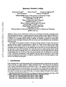
Fig. 1: Toy example of a multiple-unicast network. In quantum network (a), |·ib denotes a bit basis state and L(A1 ) is the network operation (see Section II). The network (b) and (c) is the bit and phase classical networks of the quantum network (a).

are performed on the input and output quantum systems of the n-use of the network, respectively. On the other hand, differently from [16], our code can be implemented without any manipulation of the network operations and any classical communication. Moreover, our code makes no information leakage asymptotically from a sender Si to the receivers other than Ti because the correctness of the transmitted state guarantees no information leakage [1]. To discuss the achievable rate by our code, we consider the situation that the input states of all senders are the bit basis states. Then, our network can be considered as a classical network, called bit classical network, because a bit basis state is transformed to another bit basis state by our quantum node operations. In the bit classical network, we assume that when the inputs of the senders other than Si are to zero, the transmission rate from Si to Ti is mi , which is the same as the number of outgoing edges of Si and incoming edges of Ti . Also, when we define the interference rate by the rate of the transmitted information to Ti from the senders other than Si , we assume that the interference rate to Ti is at most ai in the bit classical network. In the same way, in case that the input states of all senders are set to the phase basis states (defined in Section II), we call the network as phase classical network. In the phase classical network, we also assume that the transmission rate from Si to Ti is mi when the inputs of the senders other than Si are zero. Also, the interference rate to Ti is at most a′i in the phase classical network. Under these constraints, if ai + a′i < mi , our code achieves the rate mi − ai − a′i quantum communication from Si to Ti asymptotically. To help the understanding of the rates described above, we explain the achievable transmission rate from S1 to T1 in the network in Fig. 1. The bit and the phase classical networks (Fig. 1b and Fig. 1c) are determined from the quantum network (Fig. 1a) (see Section II). When X1′ = X2′ = Y1′ = Y2′ = 0, the transmission rates from S1 to T1 are 2 for both networks, i.e., m1 = 2, which is also the number of outgoing edges of S1 and incoming edges of T1 . Also, the interference rates from S2 to T1 are 1 and 0 for the bit and the phase classical networks, respectively. On this network, if our code from S1 to T1 with the rates (m1 , a1 , a′1 ) = (2, 1, 0) is constructed, the conditions a1 ≥ 1, a′1 ≥ 0 and a1 + a′1 < m1 are satisfied, and therefore our code implements the rate m1 − a1 − a′1 = 1 quantum transmission from S1 to T1 asymptotically. In the practical sense, our code can cope with the node malfunctions in the following case: on the multiple-unicast network with quantum invertible linear operations, the network operations are well-determined so that there is no interference between all sender-receiver pairs, but three broken nodes apply quantum invertible linear operations different from the determined ones. Moreover, let the transmission rate m1 without interferences from S1 to T1 be 100 and the number of outgoing edges of the three broken nodes be 4. In this case, 3 × 4 = 12 outgoing edges of the three broken nodes transmit the unexpected information which implies the bit (phase) interference rate is at most 12. Therefore, by our code with m1 = 100 and a1 , a′1 > 12, the sender S1 can transmit quantum states to the

receiver T1 correctly with the rate 100 − a1 − a′1 < 76 by asymptotically many uses of the network. The remaining of this paper is organized as follows. Section II introduces the formal description of the quantum multiple-unicast network with quantum invertible linear operations. Section III gives the main results of this paper. Based on the preliminaries in Section IV, Section V concretely constructs our code with the free use of negligible rate shared randomness. The encoder and decoder of our code is given in this section. Section VI analyzes the correctness of the code in Section V. Then, Section VII constructs our code without the assumption of shared randomness by attaching the secret and correctable communication protocol [11] to the code given in Section V, which proves the main result given in Section III. Section VIII gives several examples of the network that our code can be applied. Section IX is the conclusion of this paper. II. Q UANTUM N ETWORK

WITH I NVERTIBLE

L INEAR O PERATIONS

Our code is designed on the quantum network which is a generalization of a classical multiple-unicast network. In this section, we first introduce the multiple-unicast network with classical invertible linear operations and generalize this network as a network with quantum invertible linear operations. The node operations introduced in this section are identical to the operations in [17, Section II]. A. Classical Network with Invertible Linear Operations First, we describe the multiple-unicast network with classical invertible linear operations. The network topology is given as a directed Graph G = (V, E). The r senders and r receivers are given as r source nodes S1 , . . . , Sr and r terminal nodes T1 , . . . , Tr . The sender Si has mi outgoing edges and the receiver Ti has mi incoming edges. Define m := m1 + · · · + mr . The intermediate nodes are numbered from 1 to c (= |V | − 2r ) accordingly to the order of the transmission. The intermediate node numbered t has the same number kt of incoming and outgoing edges where 1 ≤ kt ≤ m. Next, we describe the transmission and the operations on this network. Each edge sends an element of the finite field Fq where q is a power of a prime number p. The t-th node operation is described as an invertible linear operation At from the information on kt incoming edges to that of kt outgoing edges. Since node operations are . For the network operation K , invertible linear, the entire network operation is written as K = Ac · · · A1 ∈ Fm×m q we introduce the following notation:   K1,1 K1,2 · · · K1,r K2,1 K2,2 · · · K2,r    m ×m K :=  . ..  , Ki,j ∈ Fq i j . ..   .. . . Kr,1

Kr,2 · · ·

Kr,r

Then, Ki,j is the network operation from Si to Tj . We assume rank Ki,i = mi which means the information from Si to Ti is completely transmitted if there is no interference. mi mr 1 When the network inputs by senders S1 , . . . , Sr are x1 ∈ Fm q , . . . , xr ∈ Fq , the output yi ∈ Fq at the receiver Ti (i = 1, . . . , r ) is written as yi =

r X

Ki,j xj = Ki,i xi + Kic zic ,

(1)

j=1

i ×(m−mi ) Kic :=[Ki,1 · · · Ki,i−1 Ki,i+1 · · · Ki,r ] ∈ Fm , q

T T T T m−mi . zic :=[xT 1 · · · xi−1 xi+1 · · · xr ] ∈ Fq

The second term Kic zic of (1) is called the interference to Ti , and rank Kic is called the rate of the interference to Ti .

1 ×n Consider the n-use of the above network. When the inputs by senders S1 , ..., Sr are X1 ∈ Fm , . . . , Xr ∈ q m ×n the output Yi ∈ Fq i at the receiver Ti (i = 1, . . . , r ) is

r ×n Fm , q

Yi =

r X

Ki,j Xj = Ki,i Xi + Kic Zic ,

j=1

T T Z :=[X1T · · · Xi−1 Xi+1 · · · XrT ]T ∈ Fq(m−mi )×n . ic

B. Quantum Network with Invertible Linear Operations We generalize the multiple-unicast network with classical invertible linear operations to the network with quantum invertible linear operations. In this quantum network, the network topology is the same graph G = (V, E). Each edge transmits a quantum system H which is q -dimensional Hilbert space spanned by the bit basis {|xib }x∈Fq . In n-use of the network, we treat the quantum system H⊗mi ×n spanned by the bit basis {|Xib }X∈Fqmi ×n . The sender Si sends a quantum system HSi := H⊗mi ×n and the receiver Ti receives a quantum system HTi := H⊗mi ×n To describe the quantum node operation, we define the following quantum operations. Definition 2.1 (Quantum Invertible Linear Operation): For invertible matrices A ∈ Fm×m and B ∈ Fqn×n , two q unitaries L(A) and R(B) are defined for any X ∈ Fm×n as q L(A)|Xib := |AXib ,

R(B)|Xib := |XBib .

The operations L(A) and R(B) are called quantum invertible linear operations. The t-th node operation is given as L(At ) and it is called quantum invertible linear operation. The entire network operation is written as the unitary L(K) = L(Ac · · · A1 ) = L(Ac ) · · · L(A1 ). When a state ρ on HS1 ⊗ · · · ⊗ HSr is transmitted by senders S1 , . . . , Sr , the network output σTi at HTi is written as σTi :=

Tr

T1 ,...,Ti−1 ,Ti+1 ,...,Tr

L(K)ρL(K)† ,

where TrT1 ,...,Ti−1 ,Ti+1 ,...,Tr is the partial trace on the system HT1 ⊗ . . . ⊗ HTi−1 ⊗ HTi+1 ⊗ . . . ⊗ HTr . When the input state on the network is |M ib on HS1 ⊗ · · · ⊗ HSr , this quantum network can be considered as the classical network in Subsection II-A. In the same way as the classical network, we assume rank Ki,i = mi which means Si transmits any bit basis states completely to Ti if the input states on source nodes Sj (j 6= i) are zero bit basis states. Similarly, rank Kic is called the rate of the bit interference to Ti . We can discuss the interference similarly on the phase basis {|zip }z∈Fq defined in [12, Section 8.1.2] by 1 X − tr xz |zip := √ ω |xib , q x∈Fq

2πi p

and tr y := Tr My (y ∈ Fq ) with the multiplication map My : x 7→ yx identifying the finite where ω := exp field Fq with the vector space Ftp . For the analysis of the phase basis interference, we give Lemma 2.1 which explains how node operations L(At ) are applied to the phase basis states. Lemma 2.1 ( [17, Appendix A]): Let A ∈ Fm×m and B ∈ Fqn×n be invertible matrices. For any M ∈ Fm×n , we q q have L(A)|M ip = |(AT )−1 M ip , R(B)|M ip = |M (B T )−1 ip . b := (AT )−1 . When the input state is a phase basis state |M ip on HS1 ⊗ · · ·⊗ For notational convenience, we denote A b ip . In this case, this quantum network can also HSr , the network operation L(K) is applied by L(K)|M ip = |KM b cc · · · A c1 . Then, K b i,j is defined from K b in the be considered as a classical network with network operation K = A same way as Ki,j .   b 1,1 K b 1,2 · · · K b 1,r K K b 2,1 K b 2,2 · · · K b 2,r   b i,j ∈ Fqmi ×mj , b :=  K , K  . . . . . .  . . .  b r,1 K b r,2 · · · K b r,r K b ic :=[K b i,1 · · · K b i,i−1 K b i,i+1 · · · K b i,r ]. K

TABLE I: Definitions of Information Rates Rate b i,i mi = rank Ki,i = rank K rank Kic b ic rank K ai a′i

Meaning Bit (phase) transmission rates from Si to Ti without interference Rate of interference to Ti Rate of phase interference to Ti Maximum rate of bit interference to Ti Maximum rate of phase interference to Ti

b i,i = mi . We also call rank K b ic the rate of phase Similarly to the condition rank Ki,i = mi , we also assume rank K interference to Ti . The transmission rates from Si to Ti are summarized in Table I. III. M AIN R ESULTS

In this section, we propose two main theorems of this paper. The two theorems state the existence of our code with and without negligible rate shared randomness, respectively. The codes stated in the theorems are concretely constructed in Section V and VII, respectively. The theorems are stated with respect to the completely mixed state ρmix and the entanglement fidelity Fe2 (ρ, κ) := hx|κ ⊗ ιR (|xihx|)|xi for the quantum channel κ and a purification |xi of the state ρ. Theorem 3.1: Consider the transmission from the sender Si to the receiver Ti over a quantum multiple-unicast network with quantum invertible linear operations given in Section II. Let mi be the bit and phase transmission b i,i ), and ai , a′ be the upper bounds of the bit rates from Si to Ti without interferences (mi = rank Ki,i = rank K i ′ b ic ≤ a ). When the condition ai + a′ < mi holds and and phase interferences, respectively (rank Kic ≤ ai , rank K i i the sender Si and receiver Ti can share the randomness whose rate is negligible in comparison with the block-length n, there exists a quantum network code whose rate is mi − ai − a′i and the entanglement fidelity Fe2 (ρmix , κi ) satisfies n(1 − Fe2 (ρmix , κi )) → 0 where κi is the quantum code protocol from sender Si to receiver Ti . Section V constructs the code stated in Theorem 3.1 and Section VI shows that this code has the performance in Theorem 3.1. Note that this code does not depend on the detailed network structure, but depends only on the information rates mi , ai and a′i . As explained in [17, Section III], our code has no information leakage from the condition n(1 − Fe2 (ρmix , κi )) → 0. Although Theorem 3.1 assumed the free use of the negligible rate shared randomness, it is possible to design the code of the same performance without negligible rate shared randomness as follows. The paper [11] gives the secret and correctable classical network communication protocol for the classical network with malicious attacks, when the transmission rate is more than the sum of the rate of attacks and the rate of information leakage. By applying the protocol in [11] to our quantum network with bit basis states, the negligible rate shared randomness can be generated. By this method, we have the following Theorem 3.2 and the details are explained in Section VII. Theorem 3.2: Consider the transmission from the sender Si to the receiver Ti over a quantum multiple-unicast network with quantum invertible linear operations given in Section II. Let mi be the bit and phase transmission b i,i ), and ai , a′ be the upper bounds of the bit rates from Si to Ti without interferences (mi = rank Ki,i = rank K i ′ b and phase interferences, respectively (rank Kic ≤ ai , rank Kic ≤ ai ). When ai + a′i < mi , there exists a quantum network code whose rate is mi −ai −a′i and the entanglement fidelity Fe2 (ρmix , κi ) satisfies n(1−Fe2 (ρmix , κi )) → 0 where κi is the quantum code protocol from sender Si to receiver Ti . IV. P RELIMINARIES

FOR

C ODE C ONSTRUCTION

Before code construction, we prepare the extended quantum system, notations, and CSS code used in our code. A. Extended Quantum System Although the unit quantum system for the network transmission is H, our code is constructed based on the extended quantum system H′ described below. First, dependently on the block-length n, we choose a power q ′ := q α to satisfy n · (n′ )mi /(q ′ )mi −max{ai ,ai } → 0 ′ ′ (e.g. q ′ = O(n1+(max{ai ,ai }+2)/(mi −max{ai ,ai })) ) where n′ := n/α. Let Fq′ be the α-dimensional field extension of

(Private Randomness Ui,1 )

ρi

Encoder EiSRi ,Ri

EiSRi ,Ri (ρi )

(Shared Randomness SRi )

S1

T1

Si

Ti

.. . .. .

.. .

Quantum Network Multiple-Unicast

σTi

Decoder DiSRi

DiSRi (σTi )

.. .

Sr

Tr

Fig. 2: Overview of code protocol from sender Si to receiver Ti . States ρi and DiSRi (σTi ) are in code space H′code . Fq . Similarly, let H′ := H⊗α be the quantum system spanned by {|xib }x∈Fq′ . Then, the n-use of the network over H can be considered as the n′ -use of the network over H′ . The quantum invertible linear operations (Definition as and B ′ ∈ Fqn×n 2.1) can also be defined for invertible matrices A′ ∈ Fm×m ′ q′ L′ (A)|Xib = |AXib , R′ (B)|Xib = |XBib ,

. for any X ∈ Fm×n q′

B. Notations for Quantum Systems and States in Our Code We introduce notations used in our code. By the n-use of the network, the sender Si transmits the system HSi = ′ H⊗mi ×n and the receiver Ti receives the system HTi = H⊗mi ×n , which are identical to H′⊗mi ×n . We partition ′ ′ the quantum system H′⊗mi ×n as H′A ⊗ H′B ⊗ H′C := H′⊗mi ×mi ⊗ H′⊗mi ×mi ⊗ H′⊗mi ×(n −2mi ) . Furthermore, we partition the systems H′A , H′B , H′C by ′

′

H′A = H′A1 ⊗ H′A2 ⊗ H′A3 := H′⊗ai ×mi ⊗ H′⊗(mi −ai −ai )×mi ⊗ H′⊗ai ×mi , ′

′

H′B = H′B1 ⊗ H′B2 ⊗ H′B3 := H′⊗ai ×mi ⊗ H′⊗(mi −ai −ai )×mi ⊗ H′⊗ai ×mi , ′

′

′

′

′

H′C = H′C1 ⊗ H′C2 ⊗ H′C3 := H′⊗ai ×(n −2mi ) ⊗ H′⊗(mi −ai −ai )×(n −2mi ) ⊗ H′⊗ai ×(n −2mi ) .

For states |φi ∈ H′A1 , |ψi ∈ H′A2 , and |ϕi ∈ H′A3 , the tensor product state in H′A is denoted as   |φi  |ψi  := |φi ⊗ |ψi ⊗ |ϕi ∈ H′A . |ϕi (mi −ai −a′i )×mi

The bit or phase basis state of (X, Y, Z) ∈ Faq′i ×mi × Fq′  +   X |Xib  Y  :=  |Y ib  , Z |Zib b

(2)

a′ ×m

× Fq′i i is denoted as  +   X |Xip  Y  :=  |Y ip  . Z |Zip p

(3)

We also introduce notations for the states in H′B and H′C in the same way as (2) and (3). In the following, we denote the k × l zero matrix as 0k,l .

C. CSS Code in Our Code In our code construction, we use the CSS code defined in this subsection which is similarly defined from [17, m ×(n′ −2mi ) which satisfy C1 ⊃ C2⊥ as Subsection IV-B]. Define two classical codes C1 , C2 ⊂ Fq′ i      0ai ,n′ −2mi ′ ′ ′ ′ ′ ai ×(n −2mi ) i −ai −ai )×(n −2mi )  ∈ Fqm′ i ×(n −2mi ) X2 ∈ F(m , , X ∈ F C1 :=  X2 ′ ′ 3 q q   X3    X1   ′ ′ ′ ′ i −ai −ai )×(n −2mi )  ∈ Fqm′ i ×(n −2mi ) X1 ∈ Fqa′i ×(n −2mi ) , X2 ∈ F(m C2 :=  X2 . ′ q   0a′i ,n′ −2mi (mi −ai −a′i )×(n′ −2mi )

For any [M1 ] ∈ C1 /C2⊥ where M1 ∈ Fq′

, define the quantum state |[M1 ]ib ∈ HC by     + 0ai ,n′−2mi |0ai ,n′ −2mi ib X 1  M1  + Y |[M1 ]ib := q =  |M1 ib  . ⊥ ⊥ |C2 | Y ∈C2 0a′i ,n′ −2mi |0a′i ,n′ −2mi ip b ′

′

With the above definitions, the code space is given as H′code := H′C2 = H′⊗(mi −ai −ai )×(n −2mi ) and a pure state |φi ∈ H′code is encoded as a superposition of the states |[M1 ]ib in this CSS code by   |0ai ,n′ −2mi ib  ∈ HC .  |φi |0a′i ,n′ −2mi ip V. C ODE C ONSTRUCTION

WITH

N EGLIGIBLE R ATE S HARED R ANDOMNESS

′

′

In this section, we construct our code that allows a sender Si to transmit a state ρi on H′code = H′⊗(mi −ai −ai )×(n −2mi ) correctly to a receiver Ti by n-use of the network when the encoder and decoder share the negligible rate random variable SRi := (Ri , Vi ). The encoder and decoder are defined depending on the private randomness Ui,1 owned by encoder and the randomness SRi shared between the encoder and decoder. These random variables are uniformly chosen from the (m −a )×mi × values or matrices satisfying the following respective conditions: the variable Ri := (Ri,1 , Ri,2 ) ∈ Fq′ i i (mi −a′i )×mi ′ satisfies rank Ri,1 = mi − ai and rank Ri,2 = mi − ai , the random variable Vi := (Vi,1 , . . . , Vi,4mi ) Fq ′ i ×mi i satisfies rank Ui,1 = mi . and the random variable Ui,1 ∈ Fm consists of 4mi values Vi,1 , . . . , Vi,4mi ∈ F4m q′ q′ SRi ,Ui,1 SR ,U SRi and decoder Di . Depending on SRi and Ui,1 , the encoder Ei i i,1 Next, we construct the encoder Ei ′ ′⊗mi ×n′ of the sender Si is defined as an isometry channel from Hcode to HSi = H . Depending on SRi , the decoder ′ DiSRi of the receiver Ti is defined as a TP-CP map from HTi = H′⊗mi ×n to H′code . Note that the randomness SRi is shared between the encoder and the decoder. Because SRi consists of αmi (2mi − ai − a′i + 4) elements of Fq , the size of the shared randomness SRi is sublinear with respect to n (i.e., negligible). SRi ,Ui,1

A. Encoder Ei

The encoder

H′code .

of the sender Si

SR ,U Ei i i,1

consists of three steps. In the following, we describe the encoding of the state |φi in

Ri encodes the state |φi with the CSS code defined in Subsection IV-C and Step E1 The isometry map Ui,0 ′ ′ the quantum systems HA and HB as    +   0ai ,mi + |0ai ,mi ib Ri  ⊗  Ri,2  ⊗  |φi  ∈ H′A ⊗ H′B ⊗ H′C = HSi . |φi =  |φ1 i := Ui,0 R i,1 0a′ ,m |0a′i ,mi ip i i b p

Step E2

By quantum invertible linear operation L′ (Ui,1 ), the encoder maps |φ1 i to |φ2 i := L′ (Ui,1 )|φ1 i.

Step E3 From random variable Vi = (Vi,1 , . . . , Vi,4mi ), define matrices Qi,1;j,k := (Vi,k )j , Qi,2;j,k := (Vi,mi +k )j for 1 ≤ j ≤ n′ − 2mi , 1 ≤ k ≤ mi , and Qi,3;j,k := (Vi,2mi +k )j , Qi,4;j,k := (Vi,3mi +k )j for ′ ′ Vi 1 ≤ j, k ≤ mi . With these matrices, define the matrix Ui,2 ∈ Fqn′ ×n as     Imi 0mi ,mi 0mi ,n′−2mi Imi 0mi ,mi 0mi ,n′−2mi Imi 0mi ,mi 0mi ,n′−2mi Vi ·0mi ,mi Imi 0mi ,n′−2mi· 0mi ,mi Imi QT Imi 0mi ,n′−2mi , Ui,2 := QT i,3 Qi,4 i,2 Qi,1 0n′−2mi ,mi In′−2mi 0n′−2mi ,mi 0n′−2mi ,mi In′−2mi 0n′−2mi ,mi 0n′−2mi ,mi In′−2mi

Vi where Id is the identity matrix of size d. By quantum invertible linear operation R′ (Ui,2 ), the encoder maps Vi |φ2 i to R′ (Ui,2 )|φ2 i. SRi ,Ui,1

By above three steps, the encoder Ei

SR ,U Ei i i,1

B. Decoder DiSRi of the receiver Ti

is described as an isometry map

Vi Ri : |φi 7→ R′ (Ui,2 )L′ (Ui,1 )Ui,0 |φi ∈ HSi .

Decoder DiSRi consists of two steps. In the following, we describe the decoding of the state |ψi ∈ HTi .

Vi −1 Since (Ui,2 ) can be constructed from shared randomness Vi by     Imi Imi 0mi ,mi 0mi ,n′ −2mi 0mi ,mi 0mi ,n′−2mi Imi 0mi ,mi 0mi ,n′−2mi Vi −1  ·−QT Imi 0mi ,n′−2mi , Imi −QT ) = 0mi ,mi (Ui,2 Imi 0mi ,n′−2mi· 0mi ,mi i,3 Qi,4 i,2 −Qi,1 0n′−2mi ,mi In′−2mi 0n′−2mi ,mi 0n′−2mi ,mi In′−2mi 0n′−2mi ,mi 0n′−2mi ,mi In′−2mi

Step D1

Vi † Vi −1 Vi † the decoder applies the reverse operation R′ (Ui,2 ) = R′ ((Ui,2 ) ) of Step E3 as |ψ1 i := R′ (Ui,2 ) |ψi. ′ ′ Step D2 Perform the bit and phase basis measurements on HA and HB , respectively, and let i ×mi be the respective measurement outcomes. By Gaussian elimination, find invertible matrices Oi,1 , Oi,2 ∈ Fm q′ Ri,2 ,Oi,2 Ri,1 ,Oi,1 ∈ Fqm′ i ×mi satisfying , Di,2 Di,1     0ai ,mi R ,O  , PWi,2 D Ri,2 ,Oi,2 Oi,2 =  Ri,2  . PWi,1 Di,1i,1 i,1 Oi,1 =  (4) i,2 Ri,1 0a′i ,mi

i where PW is the projection from Fm q ′ to the subspace W , the subspace Wi,1 consists of the vectors whose 1-st, . . . , ai -th elements are zero and the subspace Wi,2 consists of the vectors whose (mi − a′i + 1)-st, . . . , R ,O R ,O mi -th elements are zero. The case of non-existence of Di,1i,1 i,1 nor Di,2i,2 i,2 means decoding failure, which R ,O R ,O implies that the decoder performs no more operations. Also, when Di,1i,1 i,1 and Di,2i,2 i,2 are not determined R ,O R ,O uniquely, the decoder chooses Di,1i,1 i,1 and Di,2i,2 i,2 deterministically depending on Oi,1 , Ri,1 and Oi,2 , Ri,2 , respectively. \ R ,O R ,O R ,O R ,O Based on Di,1i,1 i,1 and Di,2i,2 i,2 found by (4), the decoder applies L′ (Di,1i,1 i,1 ) and L′ (Di,2i,2 i,2 ) consecutively to |ψ1 i, and the resultant state on Hcode is the output of Step D2. Then, Step D2 is written as the following TP-CP map DiRi : X R ,O ,O R ,O ,O DiRi (|ψ1 ihψ1 |) := Tr UD i i,1 i,2 σOi,1,Oi,2 (UD i i,1 i,2 )† ,

C1,C3 m ×mi Oi,1,Oi,2 ∈Fq′ i

R ,Oi,1,Oi,2

where the matrices UD i R ,Oi,1,Oi,2

UD i

and σOi,1,Oi,2 are defined as

\ R ,O R ,O :=L′ (Di,2i,2 i,2 )L′ (Di,1i,1 i,1 ),

with the identity operator IC on HC .

σOi,1,Oi,2 := Tr |ψ1 ihψ1 |(|Oi,1 ibb hOi,1 | ⊗ |Oi,2 ipp hOi,2 | ⊗ IC ), A,B

By above two steps, the decoder DiSRi is described as   Vi Vi † ) . ) |ψihψ|R′ (Ui,2 DiSRi (|ψihψ|) := DiRi R′ (Ui,2

Since the size of the shared randomness SRi is sublinear with respect to n, our code is implemented with negligible rate shared randomness. VI. C ORRECTNESS

OF

O UR C ODE

In this section, we confirm that our code correctly transmits the state from the sender Si to the receiver Ti . As is mentioned in Section III, we show the condition n(1 − Fe2 (ρmix , κi )) → 0 which implies the correctness of our code. First, we describe the quantum code protocol κi from Si to Ti , which is an integration of the encoding, transmission, and decoding. The encoding and decoding in κi is given by the probabilistic mixture of the code in Section V depending on the uniformly chosen random variables SRi and Ui,1 . Then, the code protocol κi is written as, for the state ρi on H′code ,     X 1 SRi ,Ui,1 SRi † κi (ρi ) := D (ρi ) ⊗ ρic L(K) , L(K) Ei Tr T1 ,...,Ti−1 ,Ti+1 ,...,Tr N i SRi ,Ui,1

where ρic is the state in HS1 ⊗ · · · ⊗ HSi−1 ⊗ HSi+1 ⊗ · · · ⊗ HSr of senders other than Si , and N := q ′ 4mi + |{Ui,1 ∈ (m −a )×mi (m −a′ )×mi i ×mi | rank Ui,1 = mi }| + |{Ri,1 ∈ Fq′ i i | rank Ri,1 = mi − ai }| + |{Ri,2 ∈ Fq′ i i | rank Ri,1 = Fm q′ mi − a′i }|. As explained in [17, Section IV], 1 − Fe2 (ρmix , κi ) is upper bounded by the sum of the bit error probability and the phase error probability. The bit error probability is the probability that a bit basis state |Xib ∈ H′code is sent but the bit basis measurement outcome on the decoder output is not X . In the similar way, the phase error probability is defined for the phase basis. We in that the bit and phase error probabilities  n will show oSubsections  VI-B n and ′VI-C o ′ mi ) (n )mi 1 are upper bounded by O max q1′ , (q(n , and O max , respectively. Therefore, we have ′ )mi −ai q ′ (q ′ )mi −a′i  o n1 (n′ )mi 2 . (5) n(1 − Fe (ρmix , κi )) ≤ nO max ′ , ′ m −max{a ,a′ } i i q (q ) i Since q ′ is taken in Section IV to satisfy n(1 −

Fe2 (ρmix , κi ))

n·(n′ )mi ′ (q ′ )mi −max{ai ,ai }

→ 0, the RHS of (5) converges to 0 and therefore

→ 0. This completes the proof of Theorem 3.1.

A. Notation and Lemmas for Bit and Phase Error Probabilities In this subsection, we prepare a notation and lemmas for proving the upper bounds of the bit and phase error probabilities. The upper bounds of these probabilities are shown separately in Subsections VI-B and VI-C. ′ k×(n′ −2mi ) i i with arbitrary for X ∈ Fk×n × Fq ′ × Fk×m We introduce the notation X := (X A , X B , X C ) ∈ Fk×m q′ q′ q′ positive integer k. Also, we prepare the following lemmas. Lemma 6.1: For integers d0 ≥ d1 + d2 , let W1 ⊂ Fdq′0 be a d1 -dimensional subspace and W2 ⊂ Fdq′0 be a d2 -dimensional subspace. Assume the following three conditions. (Γ1) W1 ∩ W2 = {0d0 ,1 }. (Γ2) Let m ¯ ≥ d1 + d2 . The vectors x1 , . . . , xm ¯ ∈ W1 and y1 , . . . , ym ¯ ∈ W2 satisfy span((x1 , y1 ), . . . , (xm ¯ , ym ¯ )) = W1 ⊕ W2 . ′ (Γ3) Let W1′ ⊂ Fdq′0 be a d1 -dimensional subspace and r1 , . . . , rm ¯ ∈ W1 . There exists an invertible linear map ′ A : W1 → W1 which maps

[x1 , . . . , xm ¯ ] = A[r1 , . . . , rm ¯ ].

Then, the following two statements hold.

(∆1) There exists invertible linear map D : Fdq′0 → Fdq′0 that −1 PW1′ D[(x1 , y1 ), . . . , (xm ¯ , ym ¯ )] = A [x1 , . . . , xm ¯ ] = [r1 , . . . , rm ¯ ].

(6)

(∆2) For the above linear map D , it holds for any x ∈ W1 and y ∈ W2 that PW1′ D(x, y) = A−1 x.

(7)

Proof: First, we show the item (∆1). Let W3 be a subspace of Fdq′0 that satisfies W1 ⊕ W2 ⊕ W3 = Fdq′0 . If D is defined as D|W1 = A−1 and D|W2 ⊕W3 (W2 ⊕ W3 ) = W1′⊥ , we obtain (6), i.e., (∆1) from PW1′ D((xi , yi )) = PW1′ (D|W1 (xi ) + D|W2 ⊕W3 (yi )) = A−1 xi = ri .

Next, we show the item (∆2). Since arbitrary (x, y) ∈ W1 ⊕ W2 is spanned by (x1 , y1 ), . . . , (xm ¯ , ym ¯ ), Eq. (6) implies (7), which yields (∆2). Lemma 6.2 ( [17, Lemma 7.1]): For integers da ≥ db +dc , fix a db -dimensional subspace W ⊂ Fdq′a , and randomly choose a dc -dimensional subspace R ⊂ Fdq′a with the uniform distribution. Then, we have Pr[W ∩ R = {0da ,1 }] = 1 − O(q ′

Lemma 6.3: For d ≥ d′ ,

db +dc −da −1

).

  i h 1 ′ d′ Pr rank[t1 , . . . , td ] = d t1 , . . . , td ∈ Fq′ ≥ 1 − O ′ . q

Proof: From d ≥ d′ , we have i i h h ′ ′ Pr rank[t1 , . . . , td ] = d′ t1 , . . . , td ∈ Fdq′ ≥ Pr rank[t1 , . . . , td′ ] = d′ t1 , . . . , td′ ∈ Fdq′ .

(8) ′

On the other hand, the RHS of (8) is equivalent to the probability to choose d′ independent vectors in Fdq′ :   ′ ′ i q ′ d′ q ′ d′ − q ′ h 1 q ′ d − q ′ d −1 ′ . Pr rank[t1 , . . . , td′ ] = d′ t1 , . . . , td′ ∈ Fdq′ = d′ · · · · = 1 − O ′ d′ d′ ′ ′ ′ q q q q By combining the above inequality and equality, we have the lemma. Vi defined in Step E3, we have Lemma 6.4 ( [17, Lemmas 7.2 and 7.4]): For the random matrix Ui,2  n′ −2m mi i Vi −1 A T max Pr[x ((U ) ) = 0 ] ≤ , 1,mi i,2 ′ ′ q 0n′ ,1 6=x∈Fn q′  n′ −2m mi i Vi −1 B T d . max Pr[x (( U ) ) = 0 ] ≤ 1,mi i,2 ′ n′ q 0n′ ,1 6=x∈Fq′

B. Bit Error Probability

In this subsection, we show that when arbitrary bit basis state |M ib ∈ H′code is then input state o of the sender Si , (n′ )mi 1 the original message M is correctly recovered with probability at least 1 − O max q′ , (q′ )mi −ai . Step 1: We derive a necessary condition for correct decoding of the original message M in bit basis. When arbitrary bit basis state |M ib ∈ H′code is the input state of the sender Si , the encoded state is written as   + ′ −2m 0 0 a ,m a ,n i i i i X ¯1 Ui,1   U Vi , E M EiSRi ,Ri (|M ib ) = i,2 R i,1 ¯2 ′ ′ E ¯ ∈Fmi ×mi ,E ¯ ∈Fai ×(n −2mi ) E b 1

q′

2

q′

where we ignore the normalizing factors and phase factors. ′ Note that bit state measurement on network output system HTi = H′⊗mi ×ni commutes with the decoding operation DiSRi on HTi . Therefore, in the analysis of the bit error probability, we take the method to perform bit

state measurement to HTi first, and then apply the decoding operation corresponding to DiSRi , instead of decoding first and performing bit state measurement. By performing the bit basis measurement to the network output σTi = κi (|M ibb hM |), we have the following measurement outcome Y :   0ai ,mi 0ai ,n′ −2mi ¯1  U Vi + Kic Z, E M Y = Ki,i Ui,1  i,2 Ri,1 ¯ E2 ′

′

′

i )×n ¯2 ∈ Fa′i ×(n −2mi ) and Z ∈ F(m−m ¯1 ∈ Fm′ i ×mi , E . By Step D1, Y is decoded to where E q′ q q   0ai ,mi 0ai ,n′ −2mi Vi −1 ¯1  + Kic Z(U Vi )−1 . ) = Ki,i Ui,1  Y¯ = Y (Ui,2 E M i,2 Ri,1 ¯2 E

The measurement outcome Oi,1 in Step D2 is Oi,1 = Y¯ A

  0ai ,mi  + (Kic Z(U Vi )−1 )A . = Ki,i Ui,1  i,2 Ri,1 R ,O

Since the decoder knows Oi,1 and Ri,1 , the matrix Di,1i,1 i,1 is found by Gaussian elimination to the left equation of (4) which is written as       0ai ,mi 0ai ,mi R ,O R ,O  + (Kic Z(U Vi )−1 )A  =  . PWi,1 Di,1i,1 i,1 Oi,1 = PWi,1 Di,1i,1 i,1 Ki,i Ui,1  (9) i,2 Ri,1 Ri,1 R ,Oi,1

Therefore, if the matrix Di,1i,1

derived in (9) satisfies the following equation       0ai ,n′−2mi 0ai ,n′−2mi R ,O R ,O ,  + (Kic Z(UVi )−1 )C  =  M PWi,1Di,1i,1 i,1 Y¯ C = PWi,1Di,1i,1 i,1 Ki,i Ui,1  M i,2 ¯ ¯ E2 E2

(10)

the original message M is correctly recovered. Step 2: In the next step, we show that the conditions (Γ1), (Γ2) and (Γ3) of Lemma 6.1 in the following case imply Eq. (10);    0ai ,mi   , W2 := col Kic Z(U Vi )−1 , W1′ := Wi,1, m ¯ := mi , W1 := colKi,i Ui,1  i,2 Ri,1   0ai ,mi Vi −1 A  , [y1 , . . . , ym [x1 , . . . , xm ¯ ] := (Kic Z(Ui,2 ) ) , ¯ ] := Ki,i Ui,1  Ri,1   0ai ,mi  , A := (Ki,i Ui,1 )|W ′ , (d0 , d1 , d2 ) := (mi , mi − ai , rank Kic Z), [r1 , . . . , rm ¯ ] :=  1 Ri,1

where col(T ) of the matrix T is the column space of T and Wi,1 is defined in Step D2 of Subsection V-B. Applying Lemma 6.1, we show that Eq. (10) holds if the conditions (Γ1), (Γ2) and (Γ3) are satisfied. Assume R ,O that (Γ1), (Γ2) and (Γ3) are satisfied. Then, the condition (∆1) holds which implies the existence of Di,1i,1 i,1 in (9). Moreover, (∆2) implies that for any r ∈ W1′ , y ∈ W2 and x = Ki,i Ui,1 r ∈ W1 , it holds
−1 R ,O (Ki,i Ui,1 r) = r, PW1′ Di,1i,1 i,1 (x + y) = A−1 x = (Ki,i Ui,1 )|W1′

and this yields (10).

Step step, we show that the relations (Γ1), (Γ2) and (Γ3) hold at least with probability 1 −  3: n In the′ third o (n )mi 1 O max q′ , (q′ )mi −ai , which proves the desired statement by combining the conclusion of Steps 1 and 2. Step 3-1: In this substep, we show that the probability satisfying (Γ1), (Γ2) and (Γ3) is obtained by Pr[(Γ1) ∩ (Γ2) ∩ (Γ3)] = Pr[(Γ1)] · Pr[(Γ2′ )] · Pr[(Γ2)|(Γ2′ ) ∩ (Γ1)],

(11)

where the condition (Γ2′ ) is given as Vi −1 A (Γ2′ ) rank Kic Z((Ui,2 ) ) = rank Kic Z . Eq. (11) is derived by the following reductions: (a)

(c)

(b)

Pr[(Γ1) ∩ (Γ2) ∩ (Γ3)] = Pr[(Γ1) ∩ (Γ2)] = Pr[(Γ1)] · Pr[(Γ2)|(Γ1)] (d)

= Pr[(Γ1)] · Pr[(Γ2) ∩ (Γ2′ )|(Γ1)] = Pr[(Γ1)] · Pr[(Γ2′ )|(Γ1)] · Pr[(Γ2)|(Γ2′ ) ∩ (Γ1)]

(e)

= Pr[(Γ1)] · Pr[(Γ2′ )] · Pr[(Γ2)|(Γ2′ ) ∩ (Γ1)].

The equality (a) follows from the fact that (Γ3) is always satisfied for A defined in Step 2, and (b) and (d) are trivial. (c) is obtained because (Γ2′ ) is a necessary condition for (Γ2). Since span(y1 , . . . , ym ¯ ) = W2 is a necessary condition for (Γ2) in Lemma 6.1, the condition (Γ2′ ) is also necessary for (Γ2) from Vi −1 A Vi −1 A rank Kic Z((Ui,2 ) ) = rank(Kic Z(Ui,2 ) ) = dimspan(y1 , . . . , ym ¯) Vi −1 = dim W2 = rank Kic Z(Ui,2 ) = rank Kic Z.

The equality (e) follows from the fact that (Γ1) and (Γ2′ ) are independent, which will be shown by Pr[(Γ1)|(Γ2′ )] = Pr[(Γ1)] in Step 3-2. Vi Step 3-2: In this step, we prove Pr[(Γ1)] ≥ 1 − O(1/q ′ ) and Pr[(Γ1)|(Γ2′ )] = Pr[(Γ1)]. Fix Ri,1 and Ui,2 . Then, W1 is randomly chosen d1 -dimensional subspace under uniform distribution and W2 is fixed d2 -dimensional subspace. Therefore, Lemma 6.2 can be applied with (da , db , dc , W) := (d0 , d2 , d1 , W2 ) and Pr[(Γ1)] = 1 − Vi O(q ′ d2 +d1 −d0 −1 ) ≥ 1 − O(1/q ′ ). On the other hand, since Pr[(Γ1)] does not depend on Ui,2 but Pr[(Γ2)] depends Vi ′ only on Ui,2 , we have Pr[(Γ1)|(Γ2 )] = Pr[(Γ1)]. Vi −1 A n′mi Step 3-3: In this step, we show Pr[(Γ2′ )] ≥ 1− q′m . The condition (Γ2′ ) holds if and only if xT Kic Z((Ui,2 ) ) 6= i −ai Vi −1 A mi T 01,mi for any vector x ∈ Fq′ satisfying x Kic Z 6= 01,n′ (considering Kic , Z and ((Ui,2 ) ) as linear maps on Vi −1 A row vector spaces, this is equivalent that ((Ui,2 ) ) has trivial kernel {01,n′ } for the image of Kic Z ). Therefore, T by applying Lemma 6.4 for all distinct x Kic Z which is not zero vector, we have mi mi  ′  ′ n′mi ′ ai n − 2mi ′ ′ rank Kic Z n − 2mi . ≥ 1 − q ≥ 1 − Pr[(Γ2 )] ≥ 1 − q q′ q′ q ′ mi −ai Step 3-4: Now we evaluate the probability Pr[(Γ2)|(Γ2′ ) ∩ (Γ1)] ≥ 1 − O(1/q ′ −1 ). Fix the random variable Vi Ui,2 so that (Γ2′ ) holds in the following. Define matrices Tx = [xi(1) , . . . , xi(d1 +d2 ) ], Ty = [yi(1) , . . . , yi(d1 +d2 ) ] d ×(d +d )

and T = Tx + Ty ∈ Fq′0 1 2 where i : {1, . . . , d1 + d2 } → {1, . . . , m} ¯ is an injective index function such that yi(1) , . . . , yi(d2 ) are linearly independent i.e., rank Ty = d2 . Then, we have  
Pr (Γ2)|(Γ2′ )∩(Γ1) ≥ Pr[span (xi(1) ,yi(1) ),. . . , (xi(d1 +d2 ) , yi(d1 +d2 ) ) = W1 ⊕W2 | (Γ2′ )∩(Γ1)]     (a) = Pr rank T = d1 +d2 | (Γ2′ )∩(Γ1) = Pr ker T = {0d1+d2 ,1 } | (Γ2′ ) ∩ (Γ1)   (b) = Pr ker Tx ∩ ker Ty = {0d1 +d2 ,1 } | (Γ2′ ) ∩ (Γ1) ,
where (a) follows from span (xi(1) , yi(1) ), . . . , (xi(d1 +d2 ) , yi(d1 +d2 ) ) ⊂ W1 ⊕ W2 , and (b) follows from the condition (Γ1). Since rank Tx ≤ d1 follows from its definition and the dimension of ker Ty is d1 , the condition rank Tx = d1 is a necessary condition for ker Tx ∩ ker Ty = {0d1 +d2 ,1 }. Therefore, we have   Pr ker Tx ∩ ker Ty = {0d1 +d2 ,1 } | (Γ2′ ) ∩ (Γ1)     = Pr ker Tx ∩ ker Ty | rank Tx = d1 ∩ (Γ2′ ) ∩ (Γ1) · Pr rank Tx = d1 | (Γ2′ ) ∩ (Γ1) . (12)

By applying Lemma 6.2 for (da , db , dc , W) := (d1 + d2 , d1 = dim ker Ty , d2 = dim ker  Tx , ker Ty ), the first −1 ′ ′ multiplicand of (12) equals  to 1 − O(1/q ). From Pr[rank Tx = d1 | (Γ2 ) ∩ (Γ1)] ≥ Pr rank[t1 , . . . , td1 +d2 ] = d1 | t1 , . . . , td1 +d2 ∈ Fdq′1 and Lemma 6.3, the second multiplicand of (12) is greater than or equal to 1−O(1/q ′ −1 ). Therefore, Pr[(Γ2)|(Γ2′ ) ∩ (Γ1)] ≥ 1 − O(1/q ′ −1 ). In summary, we obtain Pr[(Γ1) ∩ (Γ2) ∩ (Γ3)] = Pr[(Γ1)] · Pr[(Γ2′ )] · Pr[(Γ2)|(Γ2′ ) ∩ (Γ1)]          n 1 (n′ )mi o 1 n′mi 1 . · 1 − ′ mi −ai · 1 − O ′ = 1 − O max ′ , ′ mi −ai ≥ 1−O ′ q q q (q ) q

C. Phase Error Probability

In this subsection, the original message M ′ in the phase basis is correctly recovered with probability  nwe show′ mthato (n ) i 1 at least 1 − O max q′ , ′ mi −a′i . (q ) Step 1: We derive a necessary condition for correct decoding of the original message M ′ in phase basis. For the analysis of the phase error probability, we apply the same discussion as the bit error probability. When a phase basis state |M ′ ip ∈ H′code is the input state of sender Si , the encoded state is written as   + ¯′ E 2 X R d SRi ,Ri i,2 V ′ ′ ′ U d ¯ U i , M Ei (|M ip ) = i,2 i,1 E1 ′ mi ×mi ¯ ′ ai ×(n −2mi ) ′ ′ ′ −2m 0 0 ′ ¯ a ,n a ,m i i E1 ∈F ′ ,E2 ∈F ′ i i p q

q

where we ignore normalizing factors and phase factors. Since phase basis measurement and decoding operation DiSRi commutes, we first apply phase basis measurement, and then decode the measurement outcome for the analysis of the phase error probability. Then, the phase basis measurement outcome Y ′ on the network output of Ti is written as   ¯′ E 2 Ri,2 d Vi ¯′ b b i,i U d U M′ Y′ =K i,1  E1 i,2 + Kic Z, 0a′i ,mi 0a′i ,n′ −2mi ′

′

i )×n ¯ ′ ∈ Fa′i ×(n −2mi ) and Z ∈ F(m−m ¯ ′ ∈ Fm′ i ×mi , E . By Step D1, Y ′ is decoded to where E 2 1 q′ q q   ¯′ E 2 Ri,2 d d Vi −1 Vi −1 b i,i U d ¯′ b ic Z(U +K Y¯ ′ = Y ′ (U =K M′ i,1  E1 i,2 ) i,2 ) . 0a′i ,mi 0a′i ,n′ −2mi   Ri,2  d Vi −1 B b i,i U d b ic Z(U By Step D2, the measurement outcome Oi,2 is given as Oi,2 = Y¯ ′B = K + (K i,1  i,2 ) ) , and 0a′i ,mi Ri,2 ,Oi,2 Di,2 is found by Gaussian elimination to the right equation of (4) which is written as       R R R ,O R ,O d i,2  Vi −1 B  d b i,i U b ic Z(U PWi,2 Di,2i,2 i,2 Oi,2 = PWi,2 Di,2i,2 i,2 K + (K =  i,2  . (13) i,1  i,2 ) ) 0a′i ,mi 0a′i ,mi

R ,O

Thus, the correct estimate of M ′ is obtained when the following relation holds for Di,2i,2 i,2 derived in (13):       ¯′ ¯′ E E 2 2 R ,O R ,O d Vi −1 C  b i,i d b ic Z(U PWi,2Di,2i,2 i,2 Y¯ ′C = PWi,2Di,2i,2 i,2 K Ui,1  M ′  + (K =  M′  . (14) i,2 ) ) 0a′i ,n′−2mi 0a′i ,n′−2mi o  n ′ mi ) , Step 2: In the next step, we show that the equation (14) holds with probability at least 1−O max q1′ , (n ′ (q ′ )mi −ai which shows the desired statement by combining Step 1.

In the same way as Subsection VI-B, the conditions (Γ1), (Γ2) and (Γ3) of Lemma 6.1 in the following case imply Eq. (14);      Ri,2  d Vi −1 b d b   c W1 := col Ki,i Ui,1 , W2 := col Ki Z(Ui,2 ) , W1′ := Wi,2 , m ¯ := mi , 0a′i ,mi   d Vi −1 B b d Ri,2  , [y1 , . . . , ym b [x1 , . . . , xm ¯ ] := Ki,i Ui,1  ¯ ] := (Kic Z(Ui,2 ) ) , 0a′i ,mi   b i,i U d b ic Z),  Ri,2  , A := (K [r1 , . . . , rm (d0 , d1 , d2 ) := (mi , mi − a′i , rank K ¯ ] := i,1 )|W1′ , ′ 0ai ,mi

where Wi,2 is defined in Step D2 ofSubsection V-B. Also, o in the same way, the conditions (Γ1), (Γ2) and (Γ3) n (n′ )mi 1 holds with probability at least 1 − O max q′ , ′ mi −a′i . (q )

VII. C ODE C ONSTRUCTION W ITHOUT F REE C LASSICAL C OMMUNICATION

We show that our code in Theorem 3.1 can be implemented without the assumption of negligible rate shared randomness. The paper [11] shows the following Proposition 7.1 by constructing a secret and correctable classical communication protocol for the classical unicast linear network. Due to the relation between the phase error and the information leakage in the bit basis [13, Lemma 5.9], we find that the dimension of leaked information is a′i in the information transmission from the sender Si to the receiver Ti . We apply Proposition 7.1 to the sender-receiver pair (Si , Ti ) with c1 := ai and c2 := a′i . Therefore, the protocol of Proposition 7.1 can be implemented in our multiple-unicast network by preparing the input state of Si in the bit basis. By attaching Proposition 7.1 to our code in the above method, we can implement our code satisfying Theorem 3.2. Proposition 7.1 ( [11, Theorem 1]): Let q1 be the size of the finite field which is the information unit of the network edges. We assume the inequality c1 + c2 < c0 for the classical network where c0 is the transmission rate from the sender S to the receiver T , c1 is the rate of noise injection, and c2 is the rate of information leakage. Define q2 := q1c0 . Then, there exists a k-bit transmission protocol of block-length n1 := c0 (c0 − c2 + 1)k over Fq2 such that Perr ≤ kc0 /q2 and I(M ; E) = 0, where Perr is the error probability and I(M ; E) is the mutual information between the message M ∈ Fk2 and the leaked information E . The proof of Theorem 3.2 takes a similar method to the proof of [17, Theorem 3.2]. Proof of Theorem 3.2: To construct the code satisfying the conditions of Theorem 3.2, we generate the shared randomness SRi by Proposition 7.1 and then apply the code in Section V. To apply Proposition 7.1 in our quantum network, we prepare the input state as a bit basis state. Given a block-length n, we take q1 = q β log2 log2 n log2 n such that β = ⌊ 2 m ⌋ i.e., q2 /(log n)2 = q1mi /(log n)2 → 1, and q ′ = q α such that α = ⌊ (mi +2) ⌋ i.e., log2 q i log2 q ′ m i +2 q /n → 1. First, by the protocol of Proposition 7.1 with (c0 , c1 , c2 ) := (mi , ai , a′i ), the sender Si and the receiver Ti share the randomness SRi . Since SRi consists of mi (2mi − ai − a′i + 4) elements of Fq′ , the number of bits to be shared is       (mi + 2) log2 n ′ ′ ′ k = mi (2mi − ai − ai + 4) log2 q = mi (2mi − ai − ai + 4) log2 q log2 q   ≤ mi (mi + 2)(2mi − ai − a′i + 4) log 2 n .   log2 n → 0, and the blockThe error probability is Perr ≤ (mi /q1mi ) · ⌈mi (mi +2)(2mi −ai −a′i +4) log2 n⌉ = O (log 2 2 n) length over Fq is     2 log2 log2 n ′ ′ ′ n1 = mi (mi −ai +1)kβ ≤ mi (mi −ai +1) · mi (mi +2)(2mi −ai −ai +4) log2 n · , mi log2 q which implies n1 /n → 0. Therefore, the sharing protocol is implemented with negligible rate uses of the network.

Next, we apply the code in Section V with the extended field of size q ′ and n2 := n−n1 uses of the network. The relation n2 /n = (n − n1 )/n → 1 holds and therefore the field size q ′ satisfies n2 · (n′2 )mi /(q ′ )mi −max{ai ,ai } → 0 where n′2 := n2 /α. Thus, this code implements the code in Theorem 3.2. VIII. E XAMPLES

OF

N ETWORK

In this section, we give several network examples that our code can be applied. First, as the most trivial case, if rank Ki,i = mi and any distinct sender-receiver pairs do not interfere with each other, i.e, Ki,j (i 6= j ) are zero matrices, the network operation K is a block matrix. This is the case where each pair independently communicates. In this case, our code is implemented with the rate mi . A. Simple Network in Fig. 1 In the network in Fig. 1, the network  1 0 0 0 1 1 K= 0 0 1 0 0 0

and node operations are described as    1 0 0 0 0   0 1 0 0  1 1 0  , K b = 0 −1 1 0 , A1 = 0 1 . 0 0 0 0 1 1

When we consider the transmission from S1 to  0 c rank K1 = rank 1

T1 , the rates of bit and phase interferences are    0 0 0 b c = 0. = 1, rank K1 = rank 0 0 0

In this network, by constructing our code with (m1 , a1 , a′1 ) := (2, 1, 0), our coding protocol transmits the state of rate m1 − a1 − a′1 = 1 asymptotically from S1 to T1 . B. Network with Bit Interference from One Sender As a generalization of the network in Fig. 1, consider the case where the network consists of two sender-receiver pairs, and there is no bit interference from the sender S1 to receiver T2 . The network operation of this network can be described by L(K) with     T )−1 (K1,1 0m1 ,m2 K1,1 K1,2 b , K= K= T )−1 K T (K T )−1 (K T )−1 . 0m2 ,m1 K2,2 −(K2,2 2,2 1,1 1,2 In this network, there is no phase interference from the sender S2 to receiver T1 , and the other two rates rank K1,2 T −1 T −1 T T T )−1 K T (K T )−1 coincide from rank K and rank(K2,2 1,2 = rank K1,2 = rank(K2,2 ) K1,2 (K1,1 ) . Therefore, 1,1 1,2 ′ ′ ′ by implementing our code with ai , ai (i = 1, 2) satisfying rank K1,2 ≤ a1 , a2 < mi and a1 = a2 := 0, each sender-receiver pair can transmit the states. Moreover, we generalize the above network for arbitrary r sender-receiver pairs where the interferences are generated only from one sender S1 . In this network, the network operation is given by the unitary operator L(K) with K defined as follows:   T )−1  K 0m1 ,m2 0m1 ,m3 · · · 0m1 ,mr (K1,1 K1,2 K1,3 · · · K1,r  1,1 T −1 T T −1 T −1   0m2 ,m1 K2,2 0m2 ,m3 · · · 0m2 ,mr  b −(K2,2 ) K1,2 (K1,1 ) (K2,2 ) 0m2 ,m3 · · · 0m1 ,mr  K =  .. .. .. ..  , K =  , .. . . . . .. .. .. .. .. .   . . . . . 0mr ,m1 0mr ,m2 0mr ,m3 · · · Kr,r −(K T )−1 K T (K T )−1 0m ,m 0m ,m · · · (K T )−1 r,r

1,r

1,1

r

2

r

3

r,r

where the ranks of mi × mi matrices Ki,i are mi , resepctively. In this network, if ai , a′i (i = 1, . . . , r ) are set to a1 ≥ rank[K1,2 K1,3 · · · K1,r ], a′i ≥ rank K1,i (i = 2, . . . , r ), and a′1 = a2 = a3 = · · · = ar ≥ 0 and the condition ai + a′i < mi holds, the sender Si can send to the receiver Ti the rate mi − ai − a′i state asymptotically by our code.

C. Network with Two Way Bit Interferences In this subsection, we consider the code implementation over the network described as follows: The size q is 3, there exists two pairs (S1 , T1 ) and (S2 , T2 ) in the network, S1 , S2 , T1 , T2 are connected to three edges, and the network operation is given by L(K) of     2 0 0 2 0 0 1 0 0 1 0 0  0 1 0 0 0 0 0 1 0 0 0 0        0 0 1 0 0 0 K1,1 K1,2  0 0 1 0 0 0 b = , K = K= .   K2,1 K2,2 −2 0 0 2 0 0 −1 0 0 1 0 0  0 0 0 0 1 0  0 0 0 0 1 0 0 0 0 0 0 1 0 0 0 0 0 1

Then, differently from the previous examples, there are bit interferences both from S1 to T2 and from S2 to T1 because K1,2 and K2,1 are not zero matrix. In the above network, we construct our code for S1 to T1 with (m1 , a1 , a′1 ) := (3, 1, 1). Then, our code implements the rate mi − ai − a′i = 3 − 1 − 1 = 1 quantum communication asymptotically from the relations " # " # 100 200 b 11 = m1 = 3, rank K1c =rank 0 0 0 = 1, rank K b 1c = rank 0 0 0 = 1. rank K11 = rank K 000 000 IX. C ONCLUSION

In this paper, we have proposed a quantum network code for the multiple-unicast network with quantum invertible linear operations. As the constraints of information rates, we assumed that the bit and phase transmission rates b i,i ), the upper bounds of the bit and phase from Si to Ti without interference are mi (mi = rank Ki,i = rank K ′ ′ b interferences are ai , ai , respectively (rank Kic ≤ ai , rank Kic ≤ ai ), and ai +a′i < mi holds. Under these constraints, our code achieves the rate mi − ai − a′i quantum communication by asymptotic n-use of the network. The negligible rate shared randomness plays a crucial role in our code, and it is realized by attaching the protocol in [11]. Our code can be applied for the multiple-unicast network with the malicious adversary. When the eavesdropper attacks at most a′′i edges connected with the sender Si and the receiver Ti , if ai + a′i + 2a′′i < mi holds, our code implements the rate mi − ai − a′i − 2a′′i quantum communications asymptotically. This fact can be shown by integrating the methods in this paper and [17]. R EFERENCES [1] B. Schumacher, “Sending quantum entanglement through noisy channels,” Phys. Rev. A, 54, 2614–2628 (1996). [2] R. Ahlswede, N. Cai, S. -Y. R. Li, and R. W. Yeung, “Network information flow,” IEEE Transactions on Information Theory, vol. 46, no. 4, 1204 – 1216, 2000. [3] N. Cai and R. Yeung, “Secure network coding,” in Proceedings of 2002 IEEE International Symposium on Information Theory (ISIT), pp. 323, 2002. [4] S. Jaggi, M. Langberg, S. Katti, T. Ho, D. Katabi, M. Medard, and M. Effros, “Resilient Network Coding in the Presence of Byzantine Adversaries,” IEEE Transactions on Information Theory, vol. 54, no. 6, 2596–2603, 2008. [5] M. Hayashi, K. Iwama, H. Nishimura, R. Raymond, and S. Yamashita, “Quantum Network Coding,” in STACS 2007 SE - 52 (W. Thomas and P. Weil, eds.), vol. 4393 of Lecture Notes in Computer Science, pp. 610–621, Springer Berlin Heidelberg, 2007. [6] M. Hayashi, “Prior entanglement between senders enables perfect quantum network coding with modification,” Phys. Rev. A, vol. 76, no. 4, 40301, 2007. [7] H. Kobayashi, F. Le Gall, H. Nishimura, and M. Rötteler, “General Scheme for Perfect Quantum Network Coding with Free Classical Communication,” in Automata, Languages and Programming SE - 52 (S. Albers, A. Marchetti-Spaccamela, Y. Matias, S. Nikoletseas, and W. Thomas, eds.), vol. 5555 of Lecture Notes in Computer Science, pp. 622–633, Springer Berlin Heidelberg, 2009. [8] D. Leung, J. Oppenheim, and A. Winter, “Quantum Network Communication; The Butterfly and Beyond,” IEEE Transactions on Information Theory, vol. 56, no. 7, 3478–3490, 2010. [9] H. Kobayashi, F. Le Gall, H. Nishimura, and M. Rotteler, “Perfect quantum network communication protocol based on classical network coding,” in Proceedings of 2010 IEEE International Symposium on Information Theory (ISIT), pp. 2686–2690, 2010. [10] H. Kobayashi, F. Le Gall, H. Nishimura, and M. Rotteler, “Constructing quantum network coding schemes from classical nonlinear protocols,” in Proceedings of 2011 IEEE International Symposium on Information Theory (ISIT), pp. 109–113, 2011. [11] H. Yao, D. Silva, S. Jaggi, and M. Langberg, “Network Codes Resilient to Jamming and Eavesdropping," IEEE/ACM Transactions on Networking, vol. 22, no. 6, 1978-1987 (2014). [12] M. Hayashi, Group Representation for Quantum Theory, Springer (2017) [13] M. Hayashi, A Group Theoretic Approach to Quantum Information, Springer (2017)

[14] M. Hayashi, M. Owari, G. Kato, and N. Cai, “Secrecy and Robustness for Active Attack in Secure Network Coding,” in IEEE International Symposium on Information Theory (ISIT2017), Aachen, Germany, June, 25 – 30, 2017. pp. 1172-1177; The long version is available as arXiv: 1703.00723 (2017). [15] M. Owari, G. Kato, and M. Hayashi, “Secure Quantum Network Coding on Butterfly Network,” Quantum Science and Technology, Vol. 3, 014001 (2017). [16] G. Kato, M. Owari, and M. Hayashi, “Single-Shot Secure Quantum Network Coding for General Multiple Unicast Network with Free Public Communication,” In: Shikata J. (eds) 10th International Conference on Information Theoretic Security (ICITS2017). Lecture Notes in Computer Science, vol 10681. Springer, pp. 166-187. [17] S. Song and M. Hayashi, “Secure Quantum Network Code without Classical Communication,” arXiv: 1801.03306 (2018).