Aug 1, 2017 - and is modeled after the Quantum Toolbox in Python(QuTip). The following will explain how a problem can be defined using QuantumOptics.jl.
Bachelor Thesis
Quantum Optics Simulation using QO-Julia by
Fabian Mitterwallner supervisor Univ. Prof. Dr. Helmut Ritsch
Institute for Theoretical Physics University of Innsbruck August 1, 2017
Abstract Using numerical methods to investigate a system is an important part of modern physics. I show how the QuantumOptics.jl framework can be used to simulate an open quantum system. This is done by demonstrating in detail all the steps involved in setting up and running a simulation using a optomechanical cavity as an example. For this the Hamiltonian of the system is derived and implemented programmatically. A numerical time evolution of the master equation is used to show cooling of a mechanical oscillator, when the optomechanical system is pumped by a red shifted laser. This is done both for a system thermally isolated, and a system coupled to a heat bath. The simulated cooling happens as expected, and a clear resonant cooling behaviour is shown with regard to the frequency shift of the laser.
Contents 1. Introduction
1
2. Theoretical Foundation 2.1. Quantum Harmonic Oscillator . . . . 2.2. Optical Resonator . . . . . . . . . . 2.3. Open System Dynamics . . . . . . . 2.3.1. Density Operator Formalism . 2.3.2. Master Equation . . . . . . .
. . . . .
2 2 3 3 3 4
3. Optomechanical Oscillator 3.1. Hamiltonian . . . . . . . . . . . . . . . . . . . . . . . . . . . . . . . . . . 3.2. Interactions with the Environment . . . . . . . . . . . . . . . . . . . . .
5 6 7
. . . . .
. . . . .
4. Simulating the Problem 4.1. Introduction to QuantumOptics.jl . . . . 4.2. Defining the Problem . . . . . . . . . . . 4.2.1. Choosing a Base . . . . . . . . . 4.2.2. Defining the Operators and State 4.2.3. Time Evolution . . . . . . . . . . 4.3. Results . . . . . . . . . . . . . . . . . . . 4.3.1. Cooling . . . . . . . . . . . . . . 4.3.2. Coupling to a Heat Bath . . . . . 4.3.3. Resonant Behaviour . . . . . . .
. . . . .
. . . . . . . . .
. . . . .
. . . . . . . . .
. . . . .
. . . . . . . . .
. . . . .
. . . . . . . . .
. . . . .
. . . . . . . . .
. . . . .
. . . . . . . . .
. . . . .
. . . . . . . . .
. . . . .
. . . . . . . . .
. . . . .
. . . . . . . . .
. . . . .
. . . . . . . . .
. . . . .
. . . . . . . . .
. . . . .
. . . . . . . . .
. . . . .
. . . . . . . . .
. . . . .
. . . . . . . . .
. . . . .
. . . . . . . . .
. . . . .
. . . . . . . . .
. . . . .
. . . . . . . . .
. . . . . . . . .
9 9 9 10 11 12 12 12 14 15
5. Conclusion
17
Bibliography
18
A. QuantumOptics.jl Example
19
iii
1. Introduction In physics almost all but the most simple problems lack exact analytical solutions. In some cases reasonable approximations can be used to get good results, however not all problems lend themselves well to such methods. This is especially true in quantum physics. Modern physics uses numerical solutions and simulations to still work with such problems. There are whole branches of physics dedicated to computational and numerical methods. There are, however, also ready made toolboxes, which abstract away the algorithmic detail of finding such solutions, in favor of ease of use. On such toolbox is QuantumOptics.jl, which will be used and described more in this thesis. It is a relatively young framework for simulating open quantum systems. It is developed with the goal of being simple to use, but still be efficient.[8] I will show how the toolbox can be used by looking at one example of a quantum physical system which, as mentioned above, does not have an exact analytical solution. This system is a optomechanical cavity, in which light interacts with a mechanical vibrating object, showing interesting effects such as cooling. These are not only interesting from a theoretical point of view, but can also be realised in experiments. Some of the practical applications involve highly sensitive force and acceleration measurements.[10, 6] In chapter 2 I will first introduce some theoretical concepts from quantum physics needed in the later discussion of the problem. After which a discussion of the physical system will follow in chapter 3. Here some context is given and mechanisms and behaviours are described. The problem will also be mathematically described more closely. This involves finding the Hamiltonian describing the system, and defining the needed operators and constants to show the wanted behaviour. This is done in such a way, that it can be easily transferred to a programmatic representation, in chapter 4, which is necessary for it to be run as a simulation. In the following section some behaviour of the optomechanical cavity will be shown and the results discussed.
1
2. Theoretical Foundation First I introduce some theoretical concepts needed in later chapters. They are not intended to be full derivations of the explained properties.
2.1. Quantum Harmonic Oscillator The Hamilton operator of an object in a harmonic potential is defined as H=
pˆ2 mω 2 xˆ2 + , 2m 2
(2.1)
where xˆ is the position operator, pˆ the momentum operator, m the mass of the object and ω the frequency of the oscillator. This can be rewritten as follows: ( ) mω 2 pˆ2 H = ℏω xˆ + 2ℏ 2mℏω ((√ ) (√ ) ) mω mω pˆ pˆ i = ℏω xˆ − i √ xˆ + i √ − [ˆ x, pˆ] . 2ℏ 2ℏ 2ℏ 2mℏω 2mℏω Here [ˆ x, pˆ] := xˆpˆ − pˆxˆ is the commutator, and from the commutator relation for xˆ and pˆ we know that [ˆ x, pˆ] = iℏ. Further we can define two ladder operators as: √ ( ) mω i b= xˆ + pˆ (2.2) 2ℏ mω √ ( ) mω i † b = xˆ − pˆ (2.3) 2ℏ mω Using the commutator relation and the eqs. (2.2) and (2.3) in our Hamilton Operator we get ( ) 1 † H = ℏω b b + (2.4) 2 The eigenstate with energy En is written as |n⟩. The operator b† b is often also written as n ˆ because its expectation value equals the number of excitation n ˆ |n⟩ = n|n⟩. These states are called Fock states, and n is the number of excitations in the harmonic oscillator. For a mechanical harmonic oscillator we refer to these excitations as phonons.
2
2.2. Optical Resonator Much like for an object in a harmonic oscillator a single mode of the electro-magnetic field in a resonator can be described by the number of excitations in it. Here the excitations correspond to photons. The Hamilton of such a mode can also be defined using ladder operators called creation and annihilation operator. The finite length of the optical resonator only allows a discrete number of wavelengths to constructively interfere, causing the spectrum of a resonator to have discrete modes. The length has to be a multiple n of the half wavelength for his to happen, which gives us λn 2L L=n ⇒ λn = . 2 n The Hamilton operator then can be written as the sum of all mode energies: ( ) ∑ 1 † H= ℏωn a a + , 2 n where ωn = (πcn)/L is the frequency of the nth cavity mode and a† and a are ladder operators. To simplify notation, from now on the Hamilton operator, of both the mechanical oscillator ∑ and the optomechanical resonator, will be written without the zero point energy n (ℏωn )/2. This is possible by shifting the zero potential to this level. We therefore define ∑ H= ℏωn a† a (2.5) n
as the Hamilton of the cavity field.
2.3. Open System Dynamics An open quantum system is a system which interacts with an environment. To describe such systems using pure states and the Schrödinger equation, we also have to include the state in the environment. Assuming the environment is a lot larger then the system, and effects outside are not of interest, problems get too large and complex to describe easily.[7]
2.3.1. Density Operator Formalism To still describe open quantum systems the density operator formalism is used. A density operator for a Hilbert space is defined as ∑ ρ= pi |ψi ⟩⟨ψi |, i
3
∑ where i pi = 1. The density operator of a pure state |ψS ⟩ then is ρS = |ψS ⟩⟨ψS |. The expectation value of an observable can be calculated by ⟨A⟩ = T r (ρA) .
(2.6)
Here T r(M ) is defined as the trace of M .[5]
2.3.2. Master Equation Describing system dynamics using the Schrödinger equation only works for closed systems. To describe a open system, which interacts with a large environment we have to use the master equation. ) ∑ ( ∂ρ i 1 † 1 † † γi Ji ρJi − Ji Ji ρ − ρJi Ji = − [H, ρ] + (2.7) ∂t ℏ 2 2 i Here Ji will be called jump operators. The first term of the equation is the von Neumann equation, which is the equivalent to the Schrödinger equation for the density operator formalism. The sum on the right in the master equation describes the interaction with an environment, which leads to a non unitary time evolution.[5]
4
3. Optomechanical Oscillator Optomechanics looks at the interaction between light and matter through radiation pressure. Photons carry a momentum and when they are reflected or absorbed by an object a momentum is exchanged, leading to a pressure on the object. This effect is very small for macroscopic objects. A special category is cavity optomechanics, which uses optical resonators to increase the radiation pressure. This is achieved reflecting the light back onto the object many times. A optical resonator, also called a optical cavity, is a parallel arrangement of to mirrors, such that light, falling into the cavity, is reflected in between the two mirrors, many times. The objects experiencing the radiation pressure then are the mirrors.
Figure 3.1.: An optomechanical oscillator. (Image by Schmoele)1 Such systems are not just theoretical objects but have been realized experimentally. Some of the first experiments investigating optomechanical cavities where done by Braginsky in 1967. Since then some important applications of light and matter interactions have been developed, such as laser cooling and optical tweezers. The interaction between laser light and mirror of an interferometer also have to be taken into account when measuring gravitational waves. [3] Optomechanical cavities also have other promising applications. Because of their high sensitivity to mirror position, they are being used in highly sensitive force and acceleration measurements [10, 6]. 1
Image by Schmoele [CC BY-SA 3.0 (http://creativecommons.org/licenses/by-sa/3.0)], via Wikimedia Commons
5
The simplest model of such a system is modeled as a optical cavity where one mirror is suspended by a mechanical spring. Radiation pressure creates the interaction between the optical resonator and an mechanical oscillator, as seen in fig. 3.1. The last part of the system is the pump laser. It interacts with the cavity, by introducing new photons into it. By detuning the pump laser from the resonant frequency of the cavity mode we can also use it to couple the mechanical oscillator to the cavity, allowing it to scatter laser photons into the resonant cavity frequency and therefore exchange energy. This can be used to cool the mechanical oscillator, when the laser is red shifted (i.e. of lower frequency) relative to the cavity frequency. This can be explained in a classical picture as follows. The photons in the cavity reflect off of the mirror, which induces a force on the mirror. When the mirror moves in the positive direction, it makes the cavity longer and the resonant frequency of the cavity decreases. This, however, means the laser photons are closer to the resonant frequency and more photons enter the cavity. During this part of the oscillation the cavity extracts energy from the cavity field. As the cycle continues the mirror will begin to move in the opposite direction. Due to the fact, that the photons stay in the cavity for a finite time, the photon pressure is now higher, because the photon number is larger. During the second part of the cycle the cavity field extracts energy from the oscillator. Because the photon pressure is larger in the second half of the cycle, the net effect is that the cavity field extracts energy from the mechanical oscillator. This dampens the mechanical oscillator, which is called cooling. [9] To simulate the system, a mathematical description of the interactions is needed.
3.1. Hamiltonian The Hamilton operator for the system is made up of the optical cavity Hcav , the mechanical oscillator Hmech and the interaction between the cavity and the driving laser, as follows: H = Hcav + Hmech + Hlaser (3.1) Since we are only looking at a single mode the Hamilton operators from eq. (2.5) for the harmonic oscillator and the optical resonator are given as, H = ℏωcav a† a, H = ℏωm b† b, where ωcav is the frequency of the cavity mode and ωm is that of the mechanical oscillator. The resonant frequency of the cavity depends on the length of the cavity, which in turn depends on the position of the mirror. We define that positive displacement (x > 0) of
6
the oscillator causes the cavity to be longer. πc L(x) πc = L+x πc πc ≈ − 2x L L ω0 = ω0 − x L
ωcav (x) =
(3.2)
The laser interaction Hamilton of the laser and cavity field is given as Hlaser = ℏη(aeiωL t + a† e−iωL t ).
(3.3)
Substituting into eq. (3.1) we get H = ℏω0 a† a + ℏωm b† b − ℏ
ω0 xˆ a† a + ℏη(aeiωL t + a† e−iωL t ) L
(3.4)
The operator xˆ is the displacement operator of the mechanical oscillator, and is defined as √ ℏ xˆ = (b + b† ). (3.5) 2mωm To simulate the system we need to remove the explicit time dependence in the interaction Hamilton. This is done by transforming the problem into a reference frame rotating with the laser. Substituting eq. (3.5) into eq. (3.4) and applying the unitary transformation U = exp(iωL a† at) results in H = −ℏ∆ a† a + ℏωm b† b − ℏg (b† + b) a† a + ℏη(a + a† ) √ with ∆ = (ωL − ωcav ) and g = ω0 ℏ/(2mωm )/L. [3]
(3.6)
3.2. Interactions with the Environment As mentioned in the discussion of open systems, the Hamilton operator alone does not fully capture the behaviour of the system. In a real experimental system, there are always going to be interactions with the environment. Two such interactions are needed to describe the properties of the system looked at in this thesis. The first being photon decay in the cavity. This happens when a photon leaves the resonator. The second is a thermal coupling of the mechanical oscillator to a heat bath. To define this for our problem, we need to define the jump operators Ji of the master equation for our system. The photon decay is described by the operator being the annihilation operator of the optical resonator. Additionally a rate κ has to be defined, which is the photon decay rate and specifies how often a photon leaves the cavity on average. Jdecay = a γdecay = κ
7
The mechanical oscillator also interacts with the environment through heat exchange. Phonons of the environment can enter the oscillator mode, and phonons can also leave the mode into the environment. The rate of this interaction depends on the mean phonon density of the environment n ¯ and a coupling constant Γ, such that. Jin = a† ,
Γ n ¯ 2 Γ = (¯ n + 1) 2
γin =
Jout = a,
γout
The mean phonon number of a frequency ω, depends on the temperature of the environment and follows Bose-Einstein statistics. [3] n ¯ (ω) = exp
(
1 ℏω kB T
)
−1
In the simulation the mean phonon number will be used directly.
8
4. Simulating the Problem The theoretical formulation of the system can be translated into a programmatic representation to be simulated. The simulation comes down to solving the time dependent equations numerically, for the given Hamiltonian and jump operators. Fortunately there are pre made frameworks, which implement the numerical methods needed, one of them being QuantumOptics.jl.
4.1. Introduction to QuantumOptics.jl QuantumOptics.jl is an open source framework for open system quantum simulations. It is completely written in the programming language Julia. This is a relatively new high level programming language with the goal of being simple to write while still being efficient [4]. The framework also has the goal of being intuitive to use and having better performance than other alternatives available. It compares favorable with other frameworks in some benchmarks [8]. The version 0.4.0 of QuantumOptics.jl1 , and version 0.6.0 of Julia are used for this thesis. Since both the language and the framework are still young and actively developed, future versions might contain breaking changes necessitating changes to the described program to function. The framework is being developed by the Cavity Quantum Electrodynamics group at the University of Innsbruck, and is modeled after the Quantum Toolbox in Python(QuTip). The following will explain how a problem can be defined using QuantumOptics.jl and the steps needed. A full example can be found in appendix A. This is not a full description of the framework contents. The information given in this chapter and other information about the framework and Julia can be found in [2, 1].
4.2. Defining the Problem To formulate a given problem in QuantumOptics.jl the theoretical model described in chapter 3, has to be written in a programmatic way inside the framework. This translation can be split into multiple steps, but first the QuantumOptics.jl library has to be included into the program with: 1
using QuantumOptics
1
The framework, and its documentation, can be found at https://qojulia.org and the source code at https://github.com/qojulia/QuantumOptics.jl.
9
From now on the commands of the framework can be used. As the next step all the parameters and constant needed to describe the system have to be defined in the program, so that they can be used later. For the optomechanical cavity example this is done as follows: 2 3
ω_m = 10. ∆ = -ω_m
4 5 6 7
g = 1. η = 2. κ = 1. Here the constants are: ωm the mechanical oscillator frequency, ∆ the detuning of the laser (ωL − ωcav ), g the coupling strength of the cavity with the oscillator, η the pump strength of the laser, κ the photon decay rate. Unless stated otherwise these values will be used in the simulations.
4.2.1. Choosing a Base The framework can be used to implement many different kind of systems, and therefore supports a number of different bases. The choices include systems for: Particles
described in a PositionBasis or MomentumBasis,
Fock space where states and operators are defined using a FockBasis(n) with an upper bound n, Spins
of arbitrary spin numbers.
Others are also included and there is a interface to implement other basis sets, if needed. For the optomechanical oscillator, we need both a basis for the optical cavity b_cav, as well as the mechanical oscillator b_mech. Both problems are formulated in Fock space and therefore are defined as: 8 9
b_cav = FockBasis(5) b_mech = FockBasis(10)
10
The number passed to the FockBasis function is the cutoff, which is the highest possible energy eigenstate. Internally the framework represents states and operators as matrices. While a Fock space may have an infinite amount of possible states, the computer can only represent an finite number of them. Further more with a growing number of possible states, the size of the matrices also grows leading to lower performance, when making calculations with them. This is the reason we have to chose a cutoff. However, care has to be taken to not chose a to small number, as this can lead to numerical error in the calculation. How large the number has to be depends on the individual system. Given the basis all states and operators can now be defined.
4.2.2. Defining the Operators and State The operators needed to describe the Hamiltonian are the annihilation and creation operators, called destroy and create respectively, where these commands take the basis as an argument. The library also contains other useful operator definitions so the user mostly does not have to care about the internal representation. Since these operators have to work on the entire system, not only the subsystem their basis is defined in, the operators have to be embedded into the larger system. This is done using the ⊗ operator and the one function, which creates the identity operator. 10 11
a = destroy(b_cav) ⊗ one(b_mech) at = create(b_cav) ⊗ one(b_mech)
12 13 14
b = one(b_cav) ⊗ destroy(b_mech) bt = one(b_cav) ⊗ create(b_mech) The Hamilton operator can then be defined as in eq. (3.6) easily by using the previously defined operators and constants. It is written as:
15
H = -∆*at*a + ω_m*bt*b -g*(bt+b)*at*a + η*(at + a) For simplicity we use ℏ = 1 here. States in the Fock space can be generated using fockstate(b,n), which generates a state |n⟩ in the basis b, or coherentstate(b,α), which generates a coherent state |α⟩. For the combined system we again need to embed the states of the subsystems. Using this we define our initial state as ψ0 = |0⟩ ⊗ |2⟩ using the line:
16
ψ0 = fockstate(b_cav,0) ⊗ fockstate(b_mech,2) For working with states and operators the framework also offers some useful functions such as • expect(A,ψ), which calculates the expectation value of the operator A in the state ψ. • variance(A,ψ), which returns the variance of the operator in a given state, and • dm(ψ), returns the state ψ as a density operator.
11
4.2.3. Time Evolution Given the definitions above, the system is specified. Using this the easiest way to calculate a time evolution is using timeevolution.schroedinger(T,H,ψ) to solve the time dependent Schrödinger equation, where T is the array of times for which results are returned. For closed systems this would work, but as discussed earlier, open system dynamics follow the master equation. To fully define the master equation we need to define some jump operators J and associated constants γ. Initially the interaction with environment of interest is photon decay in the cavity. The operators and rates are then defined as: 17 18
J = [a] rates = [κ] This means, all the needed values are defined and the master equation can be solved for times in T using the following function:
19 20
T = [0:0.2:60;] tout, ρt = timeevolution.master(T, ψ0, H, J; rates=rates) The resulting ρt and tout are arrays, where ρt[i] is the density matrix at time tout[i] of the simulation.
4.3. Results Given the program described above the system can be simulated for different parameters, and its behaviour can be explored. One such behaviour mentioned earlier is the ability to cool the mechanical oscillator. This is done by choosing ∆ < 0, which means the cavity is pumped using a laser, which is red shifted relative to the cavity mode. This will first be looked at for a isolated system and then a thermally coupled system.
4.3.1. Cooling To simulate this behaviour we set ∆ = -ω_m, in the program. This will lead to resonant cooling, as seen later. The expected number of phonons in the mechanical oscillator mode can be evaluated for the states at each time step by calling: expectedN = real(expect(bt*b,ρt)) on the result ρt of the time evolution. Here expectedN is an array where the ith entry is the expected number of excitations in the oscillator at time T[i]. This is run for three different values of ∆ around ωm . The result can be seen in fig. 4.1. An exponential decay of expected phonon number can be seen. This is matches the expected cooling behaviour. While it may seem, that the phonon number goes towards 0, it does not reach such an end state. To find the actual longtime steady state, QuantumOptics.jl offers 2 functions:
12
2.00
= - _m = -1.05 _m = -0.95 _m
1.75 1.50 nm
1.25 1.00 0.75 0.50 0.25 0.00 0
10
20
30 t
40
50
60
Figure 4.1.: Resonant cavity cooling for three values of ∆ and an initial state |ψ⟩ = |0⟩ ⊗ |2⟩. The expected phonon number is exponentially damped. They all converge to ⟨nend ⟩ ≈ 8.9 · 10−4 , for this example. • steadystate.eigenvector(H,J), • steadystate.master(H,J). For small problems the eigenvector functions allows for better results, the performance for large examples becomes slow. For larger problems, the master function can still be used, as it just runs the time evolution of the master equation until an approximated convergence. For the above mentioned parameters and using steadystate.eigenvector(H,J) we reach en expected phonon number of ⟨nend ⟩ = 8.9 · 10−4 , very close to the ground state. By switching the operators in the function call to the ladder operators of the cavity we get the expected photon number over time, as in: expectedN_cav = real(expect(at*a,ρt)) The result in fig. 4.2 shows, that the photon number rises until it reaches an equilibrium of photon decay and photons entering the cavity, which decreases as the mechanical oscillator cools. The small oscillations seen have the same period as the oscillator,
13
and match the expected behaviour from the classical picture of the problem explained earlier. As the mirror oscillates the expected photon number increases and decreases during different parts of the cycle.
0.20
nc
0.15 0.10 0.05 0.00 0
10
20
30 t
40
50
60
Figure 4.2.: Expected number of photons in the cavity over time, when cooling.
4.3.2. Coupling to a Heat Bath In the model described above the mechanical oscillator is completely isolated from the environment, and therefore does not interact with it in any way. In a realistic experimental setup there will, however, always be some heat transfer from the environment to the oscillator while cooling. To simulate this behaviour, a heat bath is coupled to the mechanical oscillator in the model as described in section 3.2. This is done by redefining the jump operators J and rates. c = 0.03 meanN = 1.2 J = [a, bt, b] rates = [κ, c/2* meanN, c/2*(meanN+1)] Here c is a damping constant of the mechanical oscillator and meanN is the mean number of phonons of the heat bath. The time evolution of this system, as seen in fig. 4.3, shows that there is also an exponential decay of the expected phonon number, however it converges to a larger
14
2.00
Heat Bath Isolated
1.75 1.50 nm
1.25 1.00 0.75 0.50 0.25 0.00 0
10
20
30 t
40
50
60
Figure 4.3.: Comparison of the system dynamics, with and without coupling to a heat bath, by looking at the expected phonon number over time. result, than the isolated model. The steady state analysis of the coupled model, gives a resulting expected phonon number of ⟨nend ⟩ = 0.125. At this number the energy extracted by the cooling equals the thermal energy flowing into the system from the environment.
4.3.3. Resonant Behaviour From the results in fig. 4.1 it can also bee seen, that the rate by which the mirror is damped by the cavity depends on the detuning of the laser. The laser red shifted by ∆ = −ωm has the highest rate of damping, because here the cooling is resonant. The resonance also applies to the expected phonon number of the steady state when cooling the thermally coupled system. To show this behaviour, steady state analysis is run for a range of detuning for the laser. This is done by running:
15
1.0
nm
0.8 0.6 0.4 = 2.0 = 4.0 = 6.0
0.2 0.0
1.4
1.3
1.2
1.1
1.0 / m
0.9
0.8
0.7
0.6
Figure 4.4.: The expected phonon number of the steady state after cooling over the laser detuning, for different pump strengths η. A resonant behavior around −ωm can be seen.
n_end = [] for det = detune H_det = -det*at*a + H_mech + H_int + η*(a + at) ρ = steadystate.eigenvector(H_det, sqrt.(rates).*J) push!(n_end, real(expect(bt*b, ρ))) end The resulting n_end is then plotted against the detuning. The result for different pump strengths η can be seen in fig. 4.4. There is an obvious resonance at a red shift of ∆ = −ωm . It is also visible, that the laser pump strength influences the cooling behaviour. This effect is stronger off the resonant frequency.
16
5. Conclusion Modern toolboxes such as QuantumOptics.jl abstract away the numerical detail of simulating quantum systems as seen in chapter 4. Problems can be defined in the framework by, defining the constants, choosing a base, defining the needed operators and states and finally solving the dynamics of the system. This can be done using mathematically intuitive notation. This was shown using the example of an optomechanical cavity. The example was introduced and expected behaviour explained. After deriving the Hamilton operator the system was transferred into a programmatic representation. Using the toolbox to solve the master equation for the system, it was shown that the mechanical oscillator is damped, when the cavity is pumped by a red shifted laser, as expected. After defining the system again, this time coupled to a heat bath, a clear difference to the isolated case was shown. Additionally a resonant cooling behavior dependent on the lasers frequency was seen, and different cooling rates, depending on the pump strength have been shown.
17
Bibliography [1] Julia 0.6: Documentation. [2] QuantumOptics.jl: Documentation. [3] Markus Aspelmeyer, Tobias J Kippenberg, and Florian Marquardt. Cavity optomechanics. Reviews of Modern Physics, 86(4):1391–1452, dec 2014. [4] Jeff Bezanson, Alan Edelman, Stefan Karpinski, and Viral B. Shah. Julia: A Fresh Approach to Numerical Computing. SIAM Review, 59(1):65–98, jan 2017. [5] Heinz-Peter Breuer and Francesco Petruccione. The Theory of Open Quantum Systems. Oxford University Press, jan 2007. [6] E Gavartin, P Verlot, and T J Kippenberg. A hybrid on-chip optomechanical transducer for ultrasensitive force measurements. Nature nanotechnology, 7(June):509– 514, 2012. [7] Serge Haroche and Jean Michel Raimond. Exploring the Quantum: Atoms, Cavities, and Photons. Oxford University Press, 2010. [8] Sebastian Krämer, David Plankensteiner, Laurin Ostermann, and Helmut Ritsch. QuantumOptics.jl: A Julia framework for simulating open quantum systems. 2017. [9] Florian Marquardt, A.A. Clerk, and S.M. Girvin. Quantum theory of optomechanical cooling. Journal of Modern Optics, 55(19-20):3329–3338, nov 2008. [10] Houxun Miao, Kartik Srinivasan, and Vladimir Aksyuk. A microelectromechanically controlled cavity optomechanical sensing system. New Journal of Physics, 14, 2012.
18
A. QuantumOptics.jl Example The following example was written as part of this bachelor thesis and is meant to be added to the QuantumOptics.jl documentation as an example.
Optomechanical Cavity Cavity optomechanics describes quantum interactions between light and mechanical objects. The simples system is modeled as an optical resonator where one mirror is suspended by a spring. In this model the mechanical harmonic oscillator can couple with the optical cavity. Such a system is described by the Hamilton (for simplicity ℏ = 1 is chosen): H = −∆a† a + ωm b† b − g(b† + b)a† a + η(a + a† ) where the constants are • ωm is the frequency of the mechanical oscillator, • ∆ = ωL − ωc is the frequency by which the pump laser is detuned from the cavity frequency, • g is the coupling constant of the cavity with the oscillator and • η is the pump strength. In such a system we can cool the mechanical oscillator by red-shifted the laser by ωm relative to the cavity frequency. To simulate this behavior the needed libraries have to be imported first. using QuantumOptics using PyPlot;
19
Then all the needed constants are defined # Parameters ω_mech = 10. ∆ = -ω_mech # g η κ
Constants = 1. = 2. = 1.;
Here κ is the photon decay rate ofthe cavity. It is useful to describe the system as a pair of coupled Fockstates |n⟩ ⊗ |m⟩, where the first is the state of the cavity and the second is the state of the oscillator. For this we define the basis for each and also define their ladder operators. # Basis b_cav = FockBasis(4) b_mech = FockBasis(10) # Operators Cavity a = destroy(b_cav) ⊗ one(b_mech) at = create(b_cav) ⊗ one(b_mech) # Operators Oscillator b = one(b_cav) ⊗ destroy(b_mech) bt = one(b_cav) ⊗ create(b_mech); Using the above operators and parameters the Hamilton operator for the system can be defined as follows: # Hamilton operator H_cav = -∆*at*a + η*(a + at) H_mech = ω_mech*bt*b H_int = -g*(bt+b)*at*a H = H_cav + H_mech + H_int; Since we also want to model photon decay in the cavity we can define the needed jump operator and associated rates. We also define the initial state to be |ψ0 ⟩ = |0⟩ ⊗ |2⟩ J = [a] rates = [κ] ψ0 = fockstate(b_cav,0) ⊗ fockstate(b_mech,2);
20
Given all the above the system is fully specified, and the master equation can be solved. T = [0:0.2:60;] tout, ρt = timeevolution.master(T,ψ0,H,J;rates=rates); To see the cooling behavior mentioned above we need to look at the expected phonon number of the oscillator over time. This can be easily be plotted using the following. figure(figsize=(9, 3)) subplot(1, 2, 1) title("Mechanical Oscillator") plot(T, real(expect(bt*b, ρt))) xlabel(L"t \kappa") ylabel(L"\langle n_m \rangle") subplot(1, 2, 2) title("Cavity") plot(T, real(expect(at*a, ρt))) xlabel(L"t \kappa") ylabel(L"\langle n_{c} \rangle") tight_layout()
As expected an exponential decay of the expected phonon number in the mechanical oscillator can bee seen. The small oscillations of the cavity curve, have the same period as the mechanical oscillator. To get the final number the expected phonon number converges to, we can look at the steady state of the system. ρ_end = steadystate.eigenvector(H,sqrt.(rates).*J) println(" = ", real(expect(bt*b,ρ_end))) println(" = ", real(expect(at*a,ρ_end)))
21
⟨n_m⟩ = 0.0008899499846858123 ⟨n_c⟩ = 0.04057123454479772
System coupled to a Heat Bath The calculation up until now assumes the oscillator is thermally isolated from the environment. A more realistic setup can be simulated by coupling the mechanical oscillator to a heat bath. During the cooling process heat can therefore flow from the heat bath to the system. A harmonic oscillator coupled to a bath can be described using the following jump operators J and corresponding rates γ: Jout = b γout = 2c (¯ n + 1) c † Jin = b γin = 2 n ¯ where n ¯ is the mean phonon number of the heat bath. c = 0.03 n = 1.2
# Coupling constant # avg. phonon number of bath.
J = [a, b, bt] rates = [κ, c/2*(n+1), c/2*n] tout, ρt_bath = timeevolution.master(T, ψ0, H, J; rates=rates); Using the calculated time evolution, we can compare the expected phonon number over time, of the thermally coupled system with the isolated one. figure(figsize=(6,4)) plot(T, real(expect(bt*b, ρt_bath)), label="Heat Bath") plot(T, real(expect(bt*b, ρt)),"--", label="Isolated") xlabel(L"t \kappa") ylabel(L"\langle n_m \rangle") legend();
22
As expected the system, interacting with the heat bath converges to a higher phonon number. The resulting value can again be calculated using the functions from steadystate. ρ_end = steadystate.eigenvector(H, sqrt.(rates).*J) println(" = ", real(expect(bt*b,ρ_end))) println(" = ", real(expect(at*a,ρ_end))) ⟨n_m⟩ = 0.12540749078307115 ⟨n_c⟩ = 0.05652292664330209 Earlier we made the choice to cool using the laser red shifted by ωm . This value was chosen because the strongest cooling can be achieved here. This resonance can be visualized by finding the resulting phonon number, while cooling with different frequency shifts. The result below shows an obvious resonance around ωm . It can also be seen that the cooling depends on the pump strength η.
23
figure(figsize=(6, 4)) detune = [-12:0.3:-8;] for η = [2., 4, 6] n_end = [] for det = detune H_det = -det*at*a + H_mech + H_int + η*(a + at) ρ = steadystate.eigenvector(H_det, sqrt.(rates).*J) push!(n_end, real(expect(bt*b, ρ))) end plot(detune./ω_mech, n_end, label=L"$\eta = $\eta$") end xlabel(L"\Delta\ / \omega_m") ylabel(L"\langle n_m \rangle") legend();
24