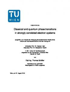
Dec 5, 2006 - Figure 4: Left potion: spectrum of Hint, Eq. (16), with h2 = 0.1, β0 = 1.3 and N = 10. Right portion: the number of d bosons (nd) probability ...
Quantum Phase Transitions in a Finite System A. Leviatan Racah Institute of Physics, The Hebrew University, Jerusalem 91904, Israel
arXiv:nucl-th/0612019v1 5 Dec 2006
Abstract A general procedure for studying finite-N effects in quantum phase transitions of finite systems is presented and applied to the critical-point dynamics of nuclei undergoing a shape-phase transition of second-order (continuous), and of first-order with an arbitrary barrier. An important issue concerning quantum phase transitions in mesoscopic systems is to understand the modifications at criticality due to their finite number of constituents. In the present contribution we study this question in connection with nuclei exemplifying a finite system undergoing a shape-phase transition. We employ the interacting boson model (IBM) [1] which describes low-lying quadrupole collective states in nuclei in terms of a system of N monopole (s) and quadrupole (d) bosons representing valence nucleon pairs. The model is based on a U (6) spectrum generating algebra and its three dynamical symmetry limits: U (5), SU (3), and O(6), describe the dynamics of stable nuclear shapes: spherical, axially-deformed, and γ-unstable deformed. A geometric visualization of the model is obtained by an intrinsic energy surface defined by the expectation value of the Hamiltonian in the coherent (intrinsic) state [2, 3] (1) (N !)−1/2 (b†c )N |0 i , √ where b†c = (1 + β 2 )−1/2 [β cos γ d†0 + β sin γ (d†2 + d†−2 )/ 2 + s† ]. For the general IBM Hamiltonian with oneand two-body interactions, the energy surface takes the form � � E(β, γ) = E0 + N (N − 1)(1 + β 2 )−2 aβ 2 − bβ 3 cos 3γ + cβ 4 . (2) | β, γ; N i =
The coefficients E0 , a, b, c involve particular linear combinations of the Hamiltonian’s parameters [4]. The quadrupole shape parameters in the intrinsic state characterize the associated equilibrium shape. Phase transitions for finite N can be studied by an IBM Hamiltonian involving terms from different dynamical symmetry chains [3]. Several works have followed this route in numerical studies of finite-N effects at criticality [5-8]. In the present contribution we consider an (approximate) analytic-oriented approach to this problem [9-11]. The nature of the phase transition is governed by the topology of the corresponding intrinsic energy surface which serves as a Landau’s potential. In a second-order phase transition, the energy surface is γ-independent and has a single minimum which changes continuously from a spherical to a deformed γ-unstable phase. At the critical-point a = b = 0 and the energy-surface acquires a flat behaviour (∼ β 4 ) for small β (justifying the use of a square-well potential in the E(5) critical-point model [12]). This is the situation encountered in the U (5)-O(6) phase transition where the critical Hamiltonian is given by i ih 1 h , ǫ = (N − 1)A . (3) Hcri = ǫ n ˆ d + A d† · d† − (s† )2 d˜ · d˜ − s2 4 Here d˜µ = (−1)µ d−µ and the dot implies a scalar product. Hcri is O(5)-invariant and involves the U (5) term n ˆd (the d-boson number operator), and the O(6)-pairing term. The intrinsic energy surface of Hcri has the form E(β)
=
1 AN (N − 1) + A N (N − 1) β 4 (1 + β 2 )−2 . 4
(4)
As shown in Fig. (1a), The global minimum at β = 0 is not well-localized and E(β) exhibits considerable instability in β. Under such circumstances fluctuations in β are large and play a significant role in the dynamics. Some of their effect can by can be taken into account by means of variation after projection of states of good O(5) ⊃ O(3) symmetry τ LM from the coherent state in Eq. (1) | ξ = 1; β, N, τ, L, M i ∝ (τ )
FN (β)
=
h
i−1/2 (τ ) FN (β) Pˆτ,LM |β, γ; N i
N X � β 2nd 1� 1 + (−1)nd −τ . 2 (N − nd )! (nd − τ )!! (nd + τ + 3)!! n =τ
(5)
d
These τ -projected states form the ground band (ξ = 1) and interpolate between the U (5) ground state, | N, nd = τ = L = 0i ≡ |sN i at β = 0 and the O(6) ground band, | N, σ = N, τ, Li at β = 1. The matrix element of Hcri (3) in these states defines the τ -projected energy surface which can be evaluated in closed form [9] i 1 h (N ) (N ) (N ) Eξ=1,τ (β) = ǫ N − S1,τ + A (1 − β 2 )2 S2,τ . (6) 4
20
E1,0(β)
E(β)
10
a) 0
0
1
2
3
b)
4
5
−4
−2
β
0 2 β
2
4
Figure 1: Energy surfaces of the critical IBM Hamiltonian Hcri (3) with N = 5 and A = 1. (a) Intrinsic energy surface E(β), Eq. (4) [solid line], and its approximation by a square-well potential [dashed line]. (b) O(5) projected energy surface Eξ=1,τ =0 (β), Eq. (6) whose global minimum is at β 2 = 0.314. (N )
(N )
(τ )
(τ )
Here Sk,τ denote the expectation values of (s† )k sk in the states (5), and are given by S1,τ = FN −1 /FN and (N )
(N )
(N −1)
S2,τ = S1,τ S1,τ
. Members of the first excited band (ξ = 2) have approximate wave functions of the form | ξ = 2; β, N, τ, Li = Nβ Pβ† | ξ = 1; β, N − 2, τ, Li
(7)
with Pβ† = [d† · d† − β 2 (s† )2 ] and Nβ a known normalization. Explicit expressions for quadrupole rates involving ˜ τ -projected states can be derived. For example, with the E2 operator T (E2) = d† s + s† d, i2 h (τ +1) (τ ) 2 (β) (β) + F F β N −1 N −1 (τ + 1) B(E2; ξ = 1; τ + 1, L′ = 2τ + 2 → ξ = 1, τ, L = 2τ ) = . (8) (τ +1) (τ ) (2τ + 5) (β) F (β) F N
N
(N )
Similar expressions for the excited-band energies Eξ=2,τ (β) and interband E2 rates are available [9]. As seen from Fig. (1), in contrast to E(β), the lowest O(5) projected energy surface Eξ=1,τ =0 (β) supports a well-defined global minimum at a certain value of β. As shown in Table 1, using this effective β-deformation in the τ -projected states provides accurate analytic estimates to the exact finite-N calculations of the critical IBM Hamiltonian which in-turn capture the essential features of the E(5) critical-point model [12] present in 134 Ba.
+ + Table 1: Excitation energies (in units of E(2+ 1,1 = 1) and B(E2) values (in units of B(E2; 21,1 → 01,0 ) = 1) 134 for the E(5) model [12], for several N=5 calculations and for the experimental data of Ba. The finite-N calculations involve the exact diagonalization of the critical IBM Hamiltonian (Hcri ) [Eq. (3)], τ -projected 2 states, L+ ξ,τ , [Eq. (5) with β = 0.314], U (5) and O(6) limits of the IBM. 134
E(5)
exact N=5
τ -projection N=5
U (5) N=5
O(6) N=5
Ba exp
E(L+ 1,2 ) E(L+ 1,3 ) E(0+ 2,0 )
2.20 3.59 3.03
2.195 3.55 3.68
2.19 3.535 3.71
2 3 2
2.5 4.5 A 1.5 B
2.32 3.66 3.57
+ B(E2; 4+ 1,2 → 21,1 ) + B(E2; 61,3 → 4+ 1,2 ) + B(E2; 0+ → 2 2,0 1,1 )
1.68 2.21 0.86
1.38 1.40 0.51
1.35 1.38 0.43
1.6 1.8 1.6
1.27 1.22 0
1.56(18) 0.42(12)
−9
5 +
2
E(β)
−9.2
0
E(β) −9.4
E2(β)
−5
E0(β)
−9.6 −10
−9.8 +
a)
0
−0.2
0
+
0
−10
−15 0.2 β
0.4
0.6
(−)
E0 (β)
b) −0.8
−0.4
0
0.4
0.8
1.2
β
Figure 2: Energy surfaces of the critical IBM Hamiltonian, Eq. (9), with κ = 0.2 and N = 10. (a) Intrinsic energy surface E(β) ≡ E(β, γ = 0), Eq. (10), [solid line]. The unmixed L = 0 and L = 2 levels are shown for illustration. (b) E(β) [solid line] as in (a), unmixed L = 0 [dashed line] and L = 2 [long dashed line] projected (−) (N ) energy surfaces, EL (β) ≡ EL (β), Eq. (12), and the lowest L = 0 eigenpotential [dot-dashed line], EL=0 (β), whose global minimum is at β = 0.591. In a first-order phase transition the intrinsic energy surface has two coexisting minima which become degenerate at the critical-point. This is the case in the U (5)-SU (3) phase transition where the critical Hamiltonian Hcri
=
ǫn ˆd − κ Q · Q
,
ǫ=
9 κ(2N − 3) 4
(9)
involves the U (5) pairing and the SU (3) quadrupole terms. The associated intrinsic energy surface E(β, γ)
� √ κ N (N − 1) β 2 � 2 , 1 − 4 2β cos 3γ + 8β 2(1 + β 2 )2
= −5κN +
(10)
1 has two degenerate minima, at β = 0 and at (β = 2√ , γ = 0). As shown in Fig. (2), the barrier separating 2 the spherical and prolate-deformed minima is extremely small and the resulting surface, E(β) ≡ E(β, γ = 0), is rather flat. This behaviour motivated the use of a square-well potential in the X(5) model [13]. Particularly relevant are states of good O(3) symmetry L projected from the intrinsic state |β, γ = 0; N i of Eq. (1),
h i−1/2 (L) ΓN (β) PˆLM |β, γ = 0; N i Z 1 � �N 1 = PL (x) dx 1 + β 2 P2 (x) N! 0
| β; N, L, M i ∝ (L)
ΓN (β)
(11)
(L)
where PL (x) is a Legendre polynomial with L even and ΓN (β) is a normalization factor. The L-projected states N | β; N, L, M i interpolate between the U (5) spherical ground state, √ |s i, with nd = τ = L = 0, at β = 0, and the SU (3) deformed ground band with (λ, µ) = (2N, 0), at β = 2. The matrix element of the Hamiltonian in these states define an L-projected energy surface which can be evaluated in closed form [10] � h i 1 � √ 2 (N ) 3 (N ) (N ) 2 2 (N ) EL (β) = ǫ N − S1,L + κ (β − 2) S2,L + 2(β − 2) Σ2,L + L(L + 1) − 2N (2N + 3) . (12) 2 4 (N )
(N )
(N )
Here S1,L , S2,L , Σ2,L are, respectively, the expectation values of n ˆ s = s† s, (s† )2 s2 , n ˆs n ˆ d in |β; N, L, M i and (N )
(L)
(L)
(N )
(N )
(N −1)
are given by S1,L = ΓN −1 (β)/ΓN (β), with S2,L = S1,L S1,L (N )
(N )
(N )
(N )
and Σ2,L = (N − 1)S1,L − S2,L . As shown in
Fig. (2b), the L = 0 projected energy surface, EL=0 (β), no-longer exhibits the double minima structure observed in the (unprojected) intrinsic energy surface. Instead, there is a minimum at β > 0, a maximum at β = 0, and a (N ) saddle point at β < 0. The L = 2 projected energy surface, EL=2 (β), has a minimum at a larger value of β > 0, (N ) (N ) and a flat shoulder near β = 0. The different behaviour of EL=2 (β) and EL=0 (β) can be attributed to the fact that the L = 2 state is well above the barrier and hence experiences essentially a flat-bottomed potential. In contrast, the two minima in the intrinsic energy surface support two coexisting spherical and deformed L = 0
+ + Table 2: Excitation energies (in units of E(2+ 1 ) = 1) and B(E2) values (in units of B(E2; 21 → 01 ) = 1) for 152 the X(5) critical-point model [13], for several N=10 calculations, and for the experimental data of Sm. The finite-N calculations involve the exact diagonalization of the critical IBM Hamiltonian [Eq. (9)], L-projected states [Eqs. (11) with β = 0.591], U (5) and SU (3) limits of the IBM.
E(4+ 1) E(6+ 1) E(8+ 1) E(10+ 1) E(0+ 2) B(E2; B(E2; B(E2; B(E2; B(E2;
+ 4+ 1 → 21 ) + + 61 → 41 ) + 8+ 1 → 61 ) + 101 → 8+ 1) + + 02 → 21 )
152
X(5)
exact N=10
L-projection N=10
U (5) N=10
SU (3) N=10
Sm exp
2.91 5.45 8.51 12.07 5.67
2.43 4.29 6.53 9.12 2.64
2.46 4.33 6.56 9.13 3.30
2 3 4 5 2
3.33 7.00 12.00 18.33 25.33
3.01 5.80 9.24 13.21 5.62
1.58 1.98 2.27 2.61 0.63
1.61 1.85 1.92 1.87 0.78
1.60 1.80 1.87 1.86 0.61
1.8 2.4 2.8 3.0 1.8
1.40 1.48 1.45 1.37 0.07
1.45 1.70 1.98 2.22 0.23
states which are subject to considerable mixing. This mixing can be studied by means of a 2 × 2 potential energy matrix, Kij , calculated in the following orthonormal L = 0 states � � 2 −1/2 |β; N, L = 0i − r12 |sN i , |Ψ1 i = |sN i , |Ψ2 i = (1 − r12 ) Kij
=
(L=0)
hΨi | Hcri |Ψj i , r12 = hsN |β; N, L = 0i = [N ! ΓN
(β)]−1/2 .
(13)
(±)
The derived eigenvalues of the matrix serve as eigenpotentials, EL=0 (β), and the corresponding eigenvectors, (±) |ΦL=0 i, are identified with the ground- and first-excited L = 0 states. The deformed states |β; N, L, M i of Eq. (11) with L > 0 are identified with excited members of the ground-band with energies given by the L(−) (N ) projected energy surface EL (β), Eq. (12). As shown in Fig. (2b), the lowest eigenpotential EL=0 (β) has a global minimum at a certain β > 0. Using this value in the L-projected states leads, as seen in Table 2, to faithful estimates to the exact finite-N calculations of the critical IBM Hamiltonian (notably for yrast states), which in-turn capture the essential features of the X(5) critical-point structure [13] relevant to 152 Sm. In a general first-order phase transition with an arbitrary barrier, the intrinsic energy energy surface of Eq. (2) satisfies a, b > 0 and b2 = 4ac at the critical-point. For γ = 0 it can be transcribed in the form [11] Ecri (β) = f (β) =
E0 + c N (N − 1)f (β) β 2 (1 + β 2 )−2 (β − β0 )2 .
(14)
As shown in Fig. 3, Ecri (β) exhibits degenerate spherical and deformed minima, at β = 0 and β = β0 = 2a b > 0. The value of β0 determines the position (β = β+ ) and height (h) of the barrier separating the two minima in a manner given in the caption. To construct a critical Hamiltonian with such an energy surface, it is convenient to resolve it into intrinsic and collective parts [4], Hcri = Hint + Hc .
(15)
The intrinsic part (Hint ) is defined to have the equilibrium condensate | β = β0 , γ = 0; N i, Eq. (1), as an exact zero-energy eigenstate and to have an energy surface as in Eq. (14) (with E0 = 0). Hint has the form h i p p �(2) i h ˜ + 7/2 (d˜d) ˜ (2) , · β0 ds (16) Hint = h2 β0 s† d† + 7/2 d† d† and by construction has the L-projected states |β = β0 ; N, Li of Eq. (11) as solvable deformed eigenstates with energy E = 0. It has also solvable�spherical eigenstates: |N, nd = τ = L = 0i ≡ |sN i and |N, nd = τ = 3, L = 3i � 2 with energy E = 0 and E = 3h2 β0 (N − 3) + 5 respectively. For large N the spectrum of Hint is harmonic, involving quadrupole vibrations about the spherical minimum with frequency ǫ, and both β and γ vibrations about the deformed minimum with frequencies ǫ = ǫβ = h2 β02 N ≫ ǫγ = 9(1 + β02 )−1 ǫβ , where the last inequality holds in the acceptable range 0 ≤ β0 ≤ 1.4. All these features are present in the exact spectrum of Hint shown in Fig. 4, which displays a zero-energy deformed (K = 0) ground band, degenerate with a spherical (nd = 0) ground state. The remaining states are either predominantly spherical, or deformed states arranged in several
0.2
f(β) 0.1
h
0
0
β+
β0
β
Figure 3: The IBM energy surface, Eq.√ (14), at the critical-point of a first-order phase transition. The position � �2 p −1+ 1+β02 1 2 1 + β and height of the barrier are β+ = −1 + and h = f (β ) = respectively. + 0 β0 4 excited K = 0 bands below the γ band. The coexistence of spherical and deformed states is evident in the right portion of Fig. 4, which shows the nd decomposition of wave functions of selected eigenstates of Hint . The “deformed” states show a broad nd distribution typical of a deformed rotor structure. The “spherical” states show the characteristic dominance of single nd components that one would expect for a spherical vibrator. The collective part (Hc ) of the full critical Hamiltonian, Eq. (15), is composed of kinetic terms which do not affect the shape of the intrinsic energy surface. It can be transcribed in the form [4] h i h i i h ˆ + E0 , (17) nd + c6 CˆO(6) − 5N nd + c5 CˆO(5) − 4ˆ Hc = c3 CˆO(3) − 6ˆ ˆ =n where N ˆd + n ˆ s . Here CˆG denotes the quadratic Casimir operator of the group G as defined in [4]. Table 3 shows the effect of different rotational terms in Hc . For the high-barrier case considered here, (β0 = 1.3, h = 0.1), the calculated spectrum resembles a rigid-rotor (E ∼ aN L(L + 1)) for the c3 -term, a rotor with centrifugal stretching (E ∼ aN L(L + 1) − bN [L(L + 1)]2 ) for the c5 -term, and a X(5)-like spectrum for the c6 -term. In all cases the B(E2) values are close to the rigid-rotor Alaga values. This behaviour is different from that√encountered when the barrier is low, e.g., for the U (5)-SU (3) case discussed above, corresponding to β0 = 1/2 2 and h ≈ 10−3 , where both the spectrum and E2 transitions are similar to the X(5) predictions. Table 3: Excitation energies and B(E2) values (in units as in Table 2) for selected terms in the critical Hamiltonian, Eqs. (15),(16),(17). The exact values are for N = 10, β0 = 1.3 and cL /h2 coefficients indicated in the Table. The entries in square brackets [...] are estimates based on the L-projected states, Eq. (11), with β = 1.327, 1.318, 1.294, determined by the global minimum of the respective lowest eigenvalue of the potential matrix, Eqs. (18),(19). The rigid-rotor and X(5) [13] predictions are shown for comparison.
E(4+ 1) E(6+ 1) E(8+ 1) E(10+ 1) E(0+ 2) B(E2; B(E2; B(E2; B(E2; B(E2;
+ 4+ 1 → 21 ) + 61 → 4+ 1) + 8+ → 6 1 1) + 101 → 8+ 1) + 0+ 2 → 21 )
c3 /h2 = 0.05
c5 /h2 = 0.1
c6 /h2 = 0.05
rotor
X(5)
3.32 6.98 11.95 18.26 6.31
[3.32] [6.97] [11.95] [18.26] [6.30]
3.28 6.74 11.23 16.58 6.01
[3.28] [6.76] [11.29] [16.69] [5.93]
2.81 5.43 8.66 12.23 4.56
[2.87] [5.63] [9.04] [12.83] [5.03]
3.33 7.00 12.00 18.33
2.91 5.45 8.51 12.07 5.67
1.40 1.48 1.46 1.37 0.005
[1.40] [1.48] [1.45] [1.37] [0.007]
1.40 1.48 1.46 1.38 0.006
[1.40] [1.48] [1.45] [1.37] [0.007]
1.45 1.53 1.50 1.41 0.19
[1.44] [1.52] [1.50] [1.55] [0.16]
1.43 1.57 1.65 1.69
1.58 1.98 2.27 2.61 0.63
"deformed"
4
E
32
31
100
Probability (%)
5
25
3 2
23 02
0
32
31
23
25
21
22
01
02
50 0 100 50 0 100 50
22
1
"spherical"
6 4 3 2 0
0 100
01 21
50
0 2 3 4 5 6 7 8 9 10 L
0
0 1 2 3 4 5 6 7 8 9 10 0 1 2 3 4 5 6 7 8 9 10
nd
nd
Figure 4: Left potion: spectrum of Hint , Eq. (16), with h2 = 0.1, β0 = 1.3 and N = 10. Right portion: the number of d bosons (nd ) probability distribution for selected eigenstates of Hint . Considerable insight of the underlying structure at the critical-point is gained by examining the 2 × 2 potential energy matrix, Kij , of Eq. (13), which reads K11
=
K22
=
2 −1/2 E0 , K12 = −c6 β 2 N (N − 1)(1 − r12 ) r12 , i h (N ) 2 2 2 −1 ˜ . E E0 + (1 − r12 ) L=0 (β) + 2c6 β N (N − 1)r12
˜ (N ) (β) is the L-projected energy surface of Hcri (15), and is given by Apart from a constant shift, E L h i h i ˜ (N ) (β) = E (N ) (β) − E0 = h2 (β − β0 )2 Σ(N ) + c3 L(L + 1) − 6D(N ) + c5 −β 4 S (N ) + D(N ) E 2,L 2,L 1,L L L 2,L i h (N ) + c6 −(1 + β 2 )2 S2,L + N (N − 1) . (N )
(N )
(N )
(18)
(19)
(N )
ˆsn ˆd, n ˆd, n ˆ d (ˆ nd −1) and n ˆ s (ˆ ns −1) respectively Here Σ2,L , D1,L , D2,L and S2,L denote the expectation values of n in |β; N, L, M i (11). As seen in Table 3, by determining the value of β in the L-projected states from the global minimum of the lowest eigenvalue of the potential matrix (18), one obtains accurate finite-N estimates to the energies and E2 rates at the critical-point. Part of the work reported was done in collaboration with J.N. Ginocchio (LANL). This work was supported by the Israel Science Foundation. REFERENCES [1] F. Iachello and A. Arima, The Interacting Boson Model, Cambridge Univ. Press, Cambridge 1987. [2] J. N. Ginocchio and M. W. Kirson, Phys. Rev. Lett. 44, 1744 (1980). [3] A. E. L. Dieperink, O. Scholten and F. Iachello, Phys. Rev. Lett. 44, 1747 (1980). [4] M. W. Kirson and A. Leviatan, Phys. Rev. Lett. 55, 2846 (1985). A. Leviatan, Ann. Phys. 179, 201 (1987). [5] R.F. Casten, D. Kusnezov and N.V. Zamfir, Phys. Rev. Lett. 82, 5000 (1999). [6] J.M. Arias, J. Dukelsky and J.E. Garc´ıa-Ramos, Phys. Rev. Lett. 91, 162502 (2003). [7] F. Iachello and N.V. Zamfir, Phys. Rev. Lett. 92, 212501 (2004). [8] D.J. Rowe, P.S. Turner and G. Rosensteel, Phys. Rev. Lett. 93, 232502 (2004). [9] A. Leviatan and J. N. Ginocchio, Phys. Rev. Lett. 90, 212501 (2003). [10] A. Leviatan, Phys. Rev. C 72, 031305 (2005). [11] A. Leviatan, (2005), in preparation. [12] F. Iachello, Phys. Rev. Lett. 85, 3580 (2000). [13] F. Iachello, Phys. Rev. Lett. 87, 052502 (2001).