Quantum Separation of Local Search and Fixed Point ... - Columbia CS

Quantum Separation of Local Search and Fixed Point Computation Xi Chen

Xiaoming Sun

Shang-Hua Teng

Institute for Advanced Study

Tsinghua University

Boston University

Abstract In this paper, we give a lower bound of Ω(n(d−1)/2 ) on the quantum query complexity for finding a fixed point of a discrete Brouwer function over grid [1 : n]d . Our bound is nearly tight, as the Grover search algorithm can be used to find a fixed point with O(nd/2 ) quantum queries. Our result establishes a nearly tight bound for the computation of d-dimensional approximate Brouwer fixed points as defined by Scarf and by Hirsch, Papadimitriou, and Vavasis. It can also be extended to the quantum model for Sperner’s Lemma in any dimensions: The quantum query complexity of finding a panchromatic cell in a Sperner coloring of a uniform triangulation of a d-dimensional simplex with nd cells is Ω(n(d−1)/2 ). For d = 2, this result improves the bound of Ω(n1/4 ) obtained by Friedl, Ivanyos, Santha, and Verhoeven. More significantly, our result provides a quantum separation of local search and fixed point computation over grid [1 : n]d , for d ≥ 4. Combining Aldous sampling with Grover search, Aaronson gave an algorithm for local search over [1 : n]d that makes O(nd/3 ) quantum queries. Thus, the quantum query model over [1 : n]d for d ≥ 4 strictly separates these two fundamental search problems.

1

Introduction

In this paper, we give a nearly tight bound on the quantum query complexity of fixed point computation over grid [1 : n]d = {1, 2, ..., n}d . Our result demonstrates a strict separation of fixed point computation and local search in the quantum query model, resolved an open question posted in [11]. We also solve the problem left open in [11] about both the randomized and quantum query complexity of discrete fixed point computation over hypercube {0, 1}n .

Motivation In various applications, we often need not only to decide whether solutions satisfying certain properties exist, but also to find a desirable solution. This family of computational problems is usually referred to as the search problem. Three fundamental types of search problems are global optimization, local search (or local optimization), and fixed point computation. In a global optimization problem, we are given an objective function h over a domain D and are asked to find a solution x ∈ D such that h(x) ≤ h(y), for all y ∈ D. In local search, we are given an objective function h over a domain D and a neighborhood function N : D → 2D . We are asked to find a solution x ∈ D such that h(x) ≤ h(y), for all y ∈ N (x). In practice, we also consider the approximation version of these problems. The fixed point computation arises in geometry, topology, game theory, and mathematical economics. Brouwer proved that every continuous map f from a three-dimensional simplex S to itself has a fixed point. In other words, there exists an x ∈ S such that f (x) = x. Brouwer’s Fixed Point Theorem can be extended to any compact, convex domain in any fixed dimension. Applying Brouwer’s theorem, Nash established that every finite, n-player game has an equilibrium point [20]. Arrow and Debreu [5] then extended the equilibrium theory to exchange markets that satisfy some very general conditions. Mathematically, fixed point computation and optimization are somewhat related. For example, one can reduce the fixed point computation to root finding: x ∈ S is a fixed point of f , if f (x) − x = 0, or kf (x) − xk = 0. If we define g(x) = kf (x) − xk, then every global optimum of g is a fixed point of f . Similarly, one can view a local optimum of h as a fixed point. For every x ∈ D, let fh (x) be a point in N (x) that minimizes h(x). Then, x is a fixed point of fh if and only if x is a local optimum of h. Of course, this reduction from local search to fixed point computation is less formal than the reduction from fixed point computation to global optimization because the function fh may not satisfy the “continuity” condition required by the Fixed Point Theorems. The following are the two fundamental complexity questions about these search problems: • Is global optimization strictly harder than fixed point computation? • Is a fixed point harder to find than a local optimum? To address these questions in the framework traditionally considered in Theoretical Computer Science, one may want to consider global optimization, local search, and fixed point computation over discrete domains. For optimization problems, it is somewhat easier to define the discrete or combinatorial analog of continuous optimization. We can consider optimizations over discrete input domains, such as over the vertices of the hypercube {0, 1}n or grid [1 : n]d . The corresponding optimization problems are: given a function h over a domain D = {0, 1}n or D = [1 : n]d , find a global or local optimum of h. In local search, for example, we may consider N (x) to be the direct neighbors of x in the hypercube or in the grid. The discrete fixed point computation is less straightforward and some inaccuracy must be introduced to ensure the existence of a solution with finite description [23, 24, 21, 16, 13]. One idea is to consider 1

approximate fixed points as suggested by Scarf [23] over a finite discretization of the convex domain, where a vertex x in the discretization is an approximate fixed point of a continuous map f if kf (x) − xk ≤ ǫ for a given ǫ > 0. Another idea is to use the direction-preserving functions (see Section 2) as introduced by Iimura, Murota, and Tamura [18] over [1 : n]d . One can also use Sperner’s definition of discrete fixed points. Sperner’s famous lemma states: Suppose that Ω is a d-dimensional simplex with vertices v1 , v2 , ..., vd+1 , and that S is a simplicial decomposition of Ω. Suppose Π assigns to each vertex of S a color from {1, 2, ..., d + 1} such that, for every vertex v of S, Π(v) 6= i if the ith component of the barycentric coordinate of v (the convex combination of v1 , v2 , ..., vd+1 to express v), is 0. Sperner’s Lemma asserts that there exists a cell in S that contains all the d + 1 colors. This fully-colored simplex cell is often referred to as a Sperner simplex of (S, Π). Now consider a Brouwer map f with Lipschitz constant L over the simplex Ω. Suppose further that the diameter of each simplex cell in S is at most ǫ/L. Then, one can define a color assignment Πf such that each fully-colored simplex in (S, Πf ) must have a vertex v satisfying kf (v) − vk ≤ Θ(ǫ). Thus, a fully-colored cell of (S, Πf ) can be viewed as an approximate, discrete fixed point of map f . The Hirsch, Papadimitriou, and Vavasis model [16] is an extension of Sperner’s Lemma from the simplex to the hypergrid [1 : n]d . Note that if the function h for optimization or the map f for fixed point computation is given by a polynomial-size circuit or a polynomial-time Turing machine, then these three problems are search problems in complexity classes FNP, PLS, and PPAD, respectively. For example, the corresponding decision problem for global optimization can be defined as: Given a polynomial description of f and a parameter W , decide whether there is a solution x such that f (x) ≥ W . Other than PLS ⊆ FNP and PPAD ⊆ FNP, the precise relations between these three classes remain unclear. In a recent paper, Chen and Teng [11] demonstrated that the randomized query model over [1 : n]d strictly separates these three fundamental search problems: Global optimization is harder than fixed-point computation, and fixed-point computation is harder than local search. In particular, they proved that given a black-box, discrete Brouwer function f from [1 : n]d to [1 : n]d , the randomized query complexity for finding an x ∈ [1 : n]d such that f (x) = x is Θ(nd−1 ). The separation statement then follows from two earlier results: A folklore theorem states that the randomized query complexity for finding a global optimum of a black-box function h from [1 : n]d to R is Θ(nd ); Aldous [2] showed that the randomized query complexity for finding a local optimum of a black-box function h from [1 : n]d to R is O(nd/2 ). They further conjectured that fixed point computation is also strictly harder than local search in the quantum query model over [1 : n]d . In particular, they conjectured that the quantum query complexity of fixed point computation over [1 : n]d is Θ(nd/2 ). Note that the upper bound of O(nd/2 ) can be easily achieved by Grover’s search algorithm. If this conjecture is true, then just like in its randomization counterpart, fixed point computation is harder than local search under the quantum query model in two or higher dimensions.

Our Contributions In this paper, we prove a lower bound of Ω(n(d−1)/2 ) on the quantum query complexity for finding a fixed point of a discrete Brouwer function over [1 : n]d . Our bound is nearly tight, as Grover’s search algorithm can be used to find a fixed point with O(nd/2 ) quantum queries. Our result gives a nearly tight bound for the computation of d-dimensional approximate Brouwer fixed points as defined by Scarf and by Hirsch, Papadimitriou, and Vavasis [16]. It can be extended to the quantum model for Sperner’s Lemma in any dimensions: The quantum query complexity of finding 2

a panchromatic cell in a Sperner coloring of a uniform triangulation of a d-dimensional simplex with nd cells is Ω(n(d−1)/2 ). For d = 2, this result improves the bound of Ω(n1/4 ) obtained by Friedl, Ivanyos, Santha, and Verhoeven [14]. Combining with a result of Aaronson [1], our result provides a quantum separation between local search and fixed point computation over grid [1 : n]d , for d ≥ 4. Using Aldous sampling with Grover search, Aaronson gave an algorithm for local search over [1 : n]d that makes O(nd/3 ) quantum queries. Thus, the quantum query model over [1 : n]d strictly separates these two fundamental search problems when d ≥ 4. We used the quantum adversary argument of Ambainis [4, 27] in our quantum lower bound proof. In particular, we hide a distribution of random, directed paths in the host grid graph (over [1 : n]d ) with a known starting vertex, and ask the algorithm to find the ending vertex of the path. This “path hiding” approach was used in [1, 27, 26] for deriving quantum lower bounds of local search. It was also used in [14] for deriving the Ω(n1/4 ) lower bound of the two-dimensional Sperner’s problem. The main difference between our work and previous works is that the paths used in previous works have some “monotone” properties. There is an increasing (or decreasing) value along the path. For any two vertices on the path, without querying other vertices we can decide which vertex appears earlier on the path. This monotone property makes it easier to derive good bound on the collision probability needed for a lower bound on local search, but limits the length of the path, making it impossible to derive tighter lower bound for fixed point computation. Instead of using “monotone” paths, we improve the path construction technique of Chen and Teng [11] in their randomized query lower bound for fixed point computation, and make it work for the quantum adversary argument. We also find an interesting connection between the two discrete domains — hypergrid [1 : n]d and hypercube {0, 1}n , which allows us to resolve a question left open in [11] on both the randomized and quantum query complexity of fixed point computation over {0, 1}n . In particular, we show that they are Ω(2n(1−ǫ) ) and Ω(2n(1−ǫ)/2 ) respectively, for all ǫ > 0.

1.1

Related Work

Hirsch, Papadimitriou and Vavasis [16] introduced the first query model for discrete fixed point computation over [1 : n]d . They proved a tight Θ(n) deterministic bound for two dimensions and an Ω(nd−2 ) deterministic lower bound in general. Chen and Deng [9] improved their bound to Θ(nd−1 ). Friedl, Ivanyos, Santha, and Verhoeven [14] considered the 2-dimensional Sperner’s problem. They proved an Ω(n1/2 ) lower bound for its randomized query complexity and an Ω(n1/4 ) lower bound for its quantum query complexity. Aaronson [1] was the first to introduce the quantum query complexity of local search over [1 : n]d √ (and also {0, 1}n ). He gave an upper bound O(nd/3 ), and a lower bound Ω(nd/4−1/2 / log n). Santha and Szegedy [22] proved a lower bound Ω(n1/4 ) for d = 2. Zhang [28] then obtained a lower bound of Ω(nd/3 ) (which is tight up to a log factor) for d ≥ 5. In the same paper, he also obtained a nearly tight quantum bound for {0, 1}n . For d = 2 and d = 3, Sun and Yao [26] eventually gave an almost optimal lower bound. Following the work of [1, 28, 26], we also use the the quantum adversary method of Ambainis [3] to establish quantum lower bound for fixed point computations. There have been several extensions of Ambainis’s method, including the weighted adversary method of Ambainis [4] and Zhang [27], the spectral method of Barnum, Saks and Szegedy [6], and the Kolmogorov complexity method of Laplante and Magniez [19]. It was shown by Spalek and Szegedy that the power of all these methods is equivalent. Recently a new adversary method with negative weights was proposed by Hoyer, Lee and Spalek [17]. We used the weighted adversary method. It might be possible that some new adversary method can be used to obtained the tight Ω(nd/2 ) quantum lower bound. 3

2

Definition of Problems

We start with some notation. We use Zdn to denote set {1, 2, ..., n}d , and Gdn to denote the natural directed graph over Zdn : edge (u, v) ∈ Gdn if there exists i ∈ [1 : d] such that |ui − vi | = 1 and uj = vj for all j : 1 ≤ j 6= i ≤ d. We use H n to denote the following directed graph over hypercube {0, 1}n : edge (u, v) ∈ H n if there exists i ∈ [1 : n] such that |ui − vi | = 1 and uj = vj for all j : 1 ≤ j 6= i ≤ n. We use Kn to denote the complete directed graph of size n: Its vertex set is {1, 2..., n}, and for all 1 ≤ i 6= j ≤ n, (i, j) is an edge in Kn . We let Kn⊗d denote the tensor product of d complete graphs: O O O O Kn⊗d = Kn Kn ... Kn Kn | {z } d

Kn⊗d

{1, 2, ..., n}d ;

More exactly, the vertex set of is (u, v) is a directed edge of Kn⊗d if there exists an i ∈ [1 : d] such that ui 6= vi and uj = vj for all j : 1 ≤ j 6= i ≤ d. Let G be a directed graph and P be a simple directed path (we say P = v1 v2 ...vk , where k ≥ 1, is simple if for all 1 ≤ i 6= j ≤ k, vi 6= vj ) in G. Then P naturally induces a map FP from the edge set of G to {0, 1}: for all (u, v) ∈ G, FP (u, v) = 1 if (u, v) ∈ P ; and FP (u, v) = 0, otherwise. We let End(P ) denote the ending vertex of path P . Finally, let Ed = {±e1 , ±e2 , ..., ±ed } denote the set of principle unit-vectors in d-dimensions. Let k · k denote k · k∞ .

2.1

Discrete Brouwer Fixed-Points

A function f : Zdn → {0} ∪ Ed is bounded if f (x) + x ∈ Zdn for all x ∈ Zdn ; v ∈ Zdn is a zero point of f if f (v) = 0. Clearly, if F (x) = x + f (x), then v is a fixed point of F iff v is a zero point of f . Definition 2.1 (Direction-Preserving Functions). A function f from set S to {0} ∪ Ed , where S ⊂ Zd , is direction-preserving if kf (u) − f (v)k ≤ 1 for all pairs u, v ∈ S such that ku − vk ≤ 1. Following the discrete fixed-point theorem of [18], we have: For every function f : Zdn → {0} ∪ Ed , if f is both bounded and direction-preserving, then there exists v ∈ Zdn such that f (v) = 0. We refer to a bounded and direction-preserving function f over Zdn as a Brouwer function over Zdn . In the query model, one can only access f by asking queries of the form: “What is f (v)?” for a point v ∈ Zdn . The problem ZPd that we will study is: Given a Brouwer function f : Zdn → {0} ∪ Ed in the query model, find a zero point of f . We use QQ dZP (n) to denote the quantum query complexity of problem ZPd . A description of the quantum query model can be found in [7] and [3]. In this paper, we will prove: Theorem 2.2 (Main). For all d ≥ 2 and large enough n, QQ dZP (n) = Ω(n

d−1 2

).

The problem ZPd defined here is computationally equivalent to the fixed point problems studied in [16, 12, 10, 25]. Thus, our result carries over to these FPC problems.

2.2

The End-of-Path Problems over Graphs Gdn , Kn⊗d and H n

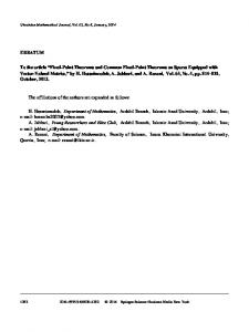
To prove Theorem 2.2, we need to introduce the following d-dimensional search problem (the End-ofPath problem over Kn⊗d ) KPd : The input is a binary string of length |Kn⊗d | (that is, the number of edges in Kn⊗d ), which encodes the map FP of a simple directed path P in Kn⊗d . P is known to start at 1 = (1, ..., 1) ∈ Zdn , and we need to find its ending vertex End(P ). We use QQ dKP (n) to denote the quantum query complexity of KPd . 4

Figure 1: End-of-Path problems over K3⊗2 , G24 and H 3 , respectively Similarly, for d ≥ 2, we define the End-of-Path problem GPd over Gdn , and use QQ dGP (n) to denote its quantum query complexity. The following reduction from GPd to ZPd was given in [11]: for any input string FP of GPd , where P is a simple path in Gdn (starting at 1), one can construct a Brouwer function f over Zd24n+7 , such that 1. Function f has exactly one fixed point v∗ ∈ Zd24n+7 . Once it is found, the ending vertex of P can be located immediately; 2. For any v ∈ Zd24n+7 , the value of f at v only depends on (at most) 4d bits of FP . By using Lemma 1 of [22], we have the following relationship between QQ dGP and QQ dZP : Lemma 2.3. For all d ≥ 2, QQ dGP (n) ≤ O(d) · QQ dZP (24n + 7). To give a lower bound for QQ dGP , we will reduce KPd to GPd+1 , and prove the following relationship between QQ dKP and QQ d+1 GP . The proof can be found in Section 5. √ Lemma 2.4. For all d ≥ 1, QQ dKP (n) ≤ O(d dn) · QQ d+1 GP (4dn + 1). Finally, in Section 3, we will prove an almost-tight lower bound (see Lemma 3.1 for an upper bound using Grover’s search algorithm) for KPd , which is also the main technical contribution of this paper: Theorem 2.5. For all d ≥ 1 and large enough n, QQ dKP (2n

+ 3) = Ω



n  d+1 2 211



.

As a result, Theorem 2.2 follows directly from Lemma 2.3, 2.4 and Theorem 2.5. Besides, as a bi-product, our work also implies an almost-tight lower bound for the End-of-Path problem HP over H n : The input is, again, a binary string of length |H n | which encodes the map FP of a simple directed path P in H n . P is known to start at 0 = (0, ..., 0) ∈ {0, 1}n and we need to find its ending vertex. Let QQ HP denote its quantum query complexity, then in Section 4, we show that Lemma 2.6. For all d ≥ 2 and n ≥ 1, QQ dGP (2n ) ≤ O(1) · QQ HP (dn). As a corollary of Lemma 2.4 and Theorem 2.5, we have Corollary 2.7. For all ǫ > 0 and large enough n, QQ HP (n) = Ω 2

5

n(1−ǫ) 2


.

An Almost-Tight Lower Bound for KPd

3

Using Grover’s search [15], we get the following upper bound for QQ dKP : √ Lemma 3.1. For all d ≥ 1, QQ dKP (n) = O( d · nd+1 ).

To prove a matching lower bound for QQ dKP , we need the following theorem from [4] and [27]:

Theorem 3.2. Let f : S → {0, 1}n1 be a partial function, where S ⊂ {0, 1}n2 . Let w : S × S → {0, 1} be a map satisfying the following condition: w(x, y) = w(y, x) for all x, y ∈ S, and w(x, y) = 0 whenever f (x) = f (y). Then the quantum query complexity of f satisfies  QQ(f ) = Ω 

where

min

x,y,i: xi 6=yi w(x,y)=1

θ(x, i) = for all x ∈ S and i ∈ [1 : n2 ].

P

s



1 1  · θ(x, i) θ(y, i)

y′ ∈S, yi′ 6=xi

P

y′ ∈S

w(x, y′ )

w(x, y′ )

d in The sketch of the lower bound proof is as follows. In Section 3.1, we build a set of hard paths Sm ⊗d d} graph K2m+3 for all d ≥ 1 and m ≥ 2. These paths induce a collection of binary strings {FP , P ∈ Sm ⊗d of length |K2m+3 |, which plays the role of S in Theorem 3.2. Naturally, f in Theorem 3.2 maps string d FP to End(P ). For some appropriate parameter β, we will define, in Section 3.2, a relation Rm,β over d d Sm × Sm . It then induces a relation over   d d FP , P ∈ Sm × FP , P ∈ Sm ,

which satisfies all the conditions for w in Theorem 3.2. Finally, we analyze θ in Section 3.3, and use Theorem 3.2 to obtain a lower bound for QQ dKP (2m + 3) = QQ(f ). ⊗d , where 1 ≤ v ≤ m for all i ∈ [1 : d]. For Notations: We use v = (v1 , ..., vd ) to denote a vertex in Km i d ≥ 2, we let Dd denote the map from Zd to Zd−1 : Dd (v) = (v1 , ..., vd−1 ). Let v ∈ Zd−1 and t ∈ Z, we use (v, t) to denote the vertex u ∈ Zd with ud = t and ui = vi for all i ∈ [1 : d − 1]. Let P = v1 v2 ...vk be a directed path, then we use P˜ = vk vk−1 ...v1 to denote the reverse of P .

3.1

Construction of the Hard Paths

d over K ⊗d . All the For all d ≥ 1 and m ≥ 2, we now construct, inductively, a set of simple paths Sm 2m+3 d start with 1 = (1, 1, ..., 1) ∈ Zd . paths in Sm

Definition 3.3 (m-connector). Every permutation π : [1 : m + 1] → [1 : m + 1] with π(1) = 1 defines a sequence of integers


C = 1 ◦ 2π(1) ◦ 2π(1) + 1 ◦ 2π(2) ◦ 2π(2) + 1 ◦ ... ◦ 2π(m + 1) ◦ 2π(m + 1) + 1 . Such a sequence C is called an m-connector. For 1 ≤ i ≤ m + 1, we also use C(i) to denote 2π(i), so

C = 1 ◦ C(1) ◦ C(1) + 1 ◦ ... ◦ C(m + 1) ◦ C(m + 1) + 1 .

We use Cm to denote the set of m-connectors.

6

Figure 2: Connectors C1 and C2 , where C1 can be r-transformed to C2 with parameters (k1 , k2 ) d when d = 1 is straight-forward: P ∈ S 1 if there is a connector C ∈ C such The construction of Sm m m that P has the following directed edges:



1, C(1) , C(1), C(1) + 1 , C(1) + 1, C(2) , ..., C(m + 1), C(m + 1) + 1 .

We also say P is generated by C. d−1 has already been constructed. A path P is in S d if it For the case when d > 1, we assume set Sm m d−1 . Here paths can be generated by a (2m + 4)-tuple (C, P1 , P2 , ..., P2m+3 ), where C ∈ Cm and Pi ∈ Sm P1 , P2 , ..., P2m+3 must satisfy the following condition: • End(P1 )=End(PC(1) ), and End(PC(i)+1 )=End(PC(i+1) ) for all i : 1 ≤ i ≤ m. ⊗d Path P is a simple path in K2m+3 which contains exactly the following edges: ⊗d with u = v = i, edge (u, v) ∈ P if • For all i ∈ {1, 3, ..., 2m + 1, 2m + 3} and vertices u, v ∈ Km d d and only if (Dd (u), Dd (v)) ∈ Pi ; ⊗d with u = v = i, edge (u, v) ∈ P if and • For all i ∈ {2, 4, ..., 2m, 2m + 2} and vertices u, v ∈ Km d d e only if (Dd (u), Dd (v)) ∈ Pi (or (Dd (v), Dd (u)) ∈ Pi , since Pei is the reverse of Pi );
• For all 1 ≤ i ≤ m + 1, (1, 1, ..., 1, C(i)), (1, 1, ..., 1, C(i) + 1) ∈ P ;
• Let v = End(P1 ), then (v, 1), (v, C(1)) ∈ P ;
• For all i : 1 ≤ i ≤ m, let v = End(PC(i)+1 ), then (v, C(i) + 1), (v, C(i + 1)) ∈ P .

3.2

d d d The Relation Rm,β over Sm × Sm

Let r ∈ Z+ be an integer such that 2r + 1 ≤ m. We first define a so-called r-transformation over Cm , the set of m-connectors. Definition 3.4. Let C1 and C2 be two m-connectors. For integers 1 ≤ k1 ≤ r and r + 1 ≤ k2 ≤ m − r, C1 can be r-transformed to C2 with parameters (k1 , k2 ) if • For 1 ≤ i ≤ k1 , C2 (k2 − k1 + i) = C1 (m − k1 + 1 + i) and C2 (m − k1 + 1 + i) = C1 (k2 − k1 + i); • For all other j ∈ [1 : m + 1], C2 (j) = C1 (j). See Fig.2 above for an example. Clearly, if connector C1 can be r-transformed to C2 , then C2 can also be r-transformed to C1 with the same parameters. Now, given a triple τ = (m, d, β) such that β ∈ (0, 32−d ] and mβ ∈ Z+ , we will inductively define d d × S d to {0, 1}. We will use it as the weight function w in a symmetric relation Rm,β = Rτ from Sm m 7

the quantum adversary argument (see Theorem 3.2). Before presenting details of the construction, we d and vertex v ∈ K ⊗d , we let introduce the following useful notations: For P ∈ Sm 2m+3 n o d , Rτ (P, P ′ ) = 1 and Nτ [P ] = Sτ [P ] ; Sτ [P ] = P ′ ∈ Sm n o Sτ [P, v] = P ′ ∈ Sτ [P ], End(P ′ ) = v and Nτ [P, v] = Sτ [P, v] ; n o ⊗d Vτ [P ] = v ∈ K2m+3 , Nτ [P, v] > 0 .

d When defining Rm,β = Rτ , we will also prove that


d Vτ [P ] = (1 − 2β)m

and

 d Vτ [P ] ⊂ 5, 7, ..., 2m + 3 ,

d for all P ∈ Sm .

(1)

1 which are generated by m-connectors C For the case when d = 1, assume P, P ′ are two paths in Sm and C ′ in Cm , respectively. Then, Rτ (P, P ′ ) = 1 iff there exist integers k1 and k2 such that C can be 1 implies (βm)-transformed to C ′ with parameters (k1 , k2 ). Clearly, this definition of Rm,β

  Vτ [P ] = C(r + 1) + 1, C(r + 2) + 1, ..., C(m − r) + 1 ⊂ 5, 7, ..., 2m + 3 ,

where r = βm, and thus, |Vτ [P ]| = (1 − 2β)m. For the case when d > 1, we use τ¯ to denote the triple (m, d − 1, β). By the inductive hypothesis, d−1 × S d−1 has already been defined, since β ∈ (0, 32−d ] ⊂ (0, 32−(d−1) ]. we assume relation Rτ¯ over Sm m Furthermore, by Eq.(1), we have
d−1  d−1 d−1 and Vτ¯ [P ] ⊂ 5, 7, ..., 2m + 3 , for all P ∈ Sm . (2) Vτ¯ [P ] = (1 − 2β)m d . Assume they are generated by (C, P , ..., P ′ ′ Let P and P ′ be two paths in Sm 1 2m+3 ) and (C , P1 , ..., ′ respectively. We set Rτ (P, P ) = 1 if the following conditions are satisfied:

′ P2m+3 ),

• Letting r = βm, there exist integers 1 ≤ k1 ≤ r and r + 1 ≤ k2 ≤ m − r such that C can be r-transformed to C ′ with parameters (k1 , k2 ); We use r1 , r2 , r3 , r4 to denote C(k2 − k1 ) + 1, C(m + 1) + 1, C(m − k1 + 1) + 1 and C(k2 ) + 1, respectively. We use l1 , l2 , l3 to denote C(m − k1 + 2), C(k2 + 1) and C(k2 − k1 + 1), respectively; • For each 1 ≤ i ≤ 3, there exists v ∈ Vτ¯ [Pri ] ∩ Vτ¯ [Pli ] such that Pr′i ∈ Sτ¯ [Pri , v], Pl′i ∈ Sτ¯ [Pli , v]; • Pr′4 ∈ Sτ¯ [Pr4 ]; • For all other j : 1 ≤ j ≤ 2m + 3, Pj′ = Pj . We now prove Eq.(1): Proof. We prove that Vτ [P ] =

[

t=C(k)+1, r+1≤k≤m−r

 Vτ¯ [Pt ] × t .

⊗d To prove this, we only need to show that, for every vertex v ∈ K2m+3 such that vd = C(k) + 1 with r + 1 ≤ k ≤ m − r and (v1 , v2 , ..., vd−1 ) ∈ Vτ¯ [Pvd ], Nτ [P, v] > 0.

8

For all i, j : 1 ≤ i 6= j ≤ m + 1, we let X Mi,j =

v∈Vτ¯ [PC(i)+1 ]∩Vτ¯ [PC(j) ]

Nτ¯ [PC(i)+1 , v] · Nτ¯ [PC(j) , v].

From Eq.(2), we have
d−1
− md−1 = 2(1 − 2β)d−1 − 1 md−1 > 0, Vτ¯ [PC(i)+1 ] ∩ Vτ¯ [PC(j) ] ≥ 2 (1 − 2β)m since β < 32−d . Therefore, Mi,j > 0 for all i, j. On the other hand, we can write Nτ [P, v] as Nτ [P, v] =

r X

k1 =1

Mk−k1 ,m−k1 +2 · Mm+1,k+1 · Mm−k1 +1,k−k1+1 · Nτ¯ [Pvd , (v1 , ..., vd−1 )] > 0,

(3)

since we assumed that (v1 , v2 , ..., vd−1 ) ∈ Vτ¯ [Pvd ]. d We now prove the following important lemma about relation Rm,β = Rτ :

Lemma 3.5. For d ≥ 1 and β ∈ (0, 32−d ] such that r = βm ∈ Z+ , let µ1 (β) = 1, then we have 1 Nτ [P, v] ≤ ≤ µd (β), µd (β) Nτ [P ′ , v′ ]

d for all P, P ′ ∈ Sm , v ∈ Vτ [P ] and v′ ∈ Vτ [P ′ ],

where µd (β) is defined inductively as follows: for d ≥ 2, µd (β) =

(µd−1 (β))7 (2 (1 − 2β)d−1 − 1)3

.

Proof. The case when d = 1 is trivial. For d > 1, suppose P is generated by (C, P1 , ..., P2m+3 ) and P ′ is ′ ′ for P and P ′ , respectively. Then, by generated by (C ′ , P1′ , ..., P2m+3 ). We similarly define Mi,j and Mi,j the inductive hypothesis and Eq.(1). we have Mi,j (µd−1 (β))2 ≤ . Mi′ ,j ′ 2(1 − 2β)d−1 − 1 The lemma follows directly by applying this inequality to every item in Eq.(3). The following lemma is easy to verify (by induction): d−1 β

Lemma 3.6. For all d ≥ 1 and β ∈ (0, 32−d ], µd (β) ≤ e32

.

d . For all i, j : 1 ≤ i 6= j ≤ m + 1, M Let P be a path in Sm i,j is defined as above, then we have the following two corollaries of Lemma 3.6.

Corollary 3.7. For all 1 ≤ i 6= j, i′ 6= j ′ ≤ m + 1, Mi,j /Mi′ ,j ′ < 2. d , N [P ]/N [P ′ ] ≤ µ (β) < 2. Corollary 3.8. For all paths P and P ′ in Sm τ τ d

9

3.3

Proof of the Lower Bound

For d ≥ 1 and β ∈ (0, 32−d ], we show that, when m is large enough (and satisfies βm ∈ Z+ ), relation d Rτ = Rm,β can serve as the weight function w in Theorem 3.2, and give us a lower bound   m  d+1 2 Ω 211

for QQd (2m + 3). ⊗d d , and vertex v ∈ K ⊗d . We introduce the Let (v1 , v2 ) be a directed edge in K2m+3 , path P ∈ Sm 2m+3 following notations: n o Sτ [P, (v1 , v2 )] = P ′ ∈ Sτ [P ], FP (v1 , v2 ) 6= FP ′ (v1 , v2 ) , Sτ [P, v, (v1 , v2 )] = Sτ [P, v] ∩ Sτ [P, (v1 , v2 )], Nτ [P, (v1 , v2 )] = Sτ [P, (v1 , v2 )] and Nτ [P, v, (v1 , v2 )] = Sτ [P, v, (v1 , v2 )]

We also define


Nτ [P, (v1 , v2 )] θτ P, (v1 , v2 ) = = Nτ [P ]

P

v∈Vτ [P ] Nτ [P, v, (v

1 , v2 )]

Nτ [P ]

.

Finally, we prove the following lemma. Theorem 2.5 then follows as a corollary of Theorem 3.2. Lemma 3.9. Let d ≥ 1 and β ∈ (0, 32−d ]. There exists a constant Ld,β such that for all m ≥ Ld,β with d satisfy βm ∈ Z+ , if P, P ′ ∈ Sm d (P, P ′ ) = Rτ (P, P ′ ) = 1 and FP (v1 , v2 ) 6= FP ′ (v1 , v2 ) Rm,β ⊗d for some edge (v1 , v2 ) ∈ K2m+3 , then



θτ P, (v , v ) · θτ P ′ , (v1 , v2 ) ≤ 1

2



211 m

d+1

.

Proof. Without loss of generality, assume FP (v1 , v2 ) = 0 and FP ′ (v1 , v2 ) = 1. We use mathematical induction on d. When d = 1, suppose P and P ′ are generated by C and C ′ , respectively, and C can be (r = βm)transformed to C ′ with parameters (k1 , k2 ). Then we have the following three cases: 1. When (v 1 , v 2 ) = (C(k2 − k1 ) + 1, C(m − k1 + 2)), then
θτ P, (v 1 , v 2 ) =


1 2 ; and θτ P ′ , (v 1 , v 2 ) ≤ 2 β(1 − 2β)m (1 − 2β)m

2. When (v 1 , v 2 ) = (C(m + 1) + 1, C(k2 + 1)), then
θτ P, (v 1 , v 2 ) =


1 2 and θτ P ′ , (v 1 , v 2 ) ≤ ; (1 − 2β)m (1 − 2β)m

3. When (v 1 , v 2 ) = (C(m − k1 + 1) + 1, C(k2 − k1 + 1)), then
θτ P, (v 1 , v 2 ) =


1 1 and θτ P ′ , (v 1 , v 2 ) = . 2 β(1 − 2β)m βm 10

Clearly, when m is large enough (e.g., set L1,β = (1 − 2β)/(2β 2 )), θτ (P, (v 1 , v 2 )) · θτ (P ′ , (v 1 , v 2 )) in the second case is greater than the other two cases, and we have  11 2

2 2 1 2 ′ 1 2 θτ P, (v , v ) · θτ P , (v , v ) ≤ < . 2 ((1 − 2β)m) m

′ When d > 1, suppose P and P ′ are generated by (C, P1 , ..., P2m+3 ) and (C ′ , P1′ , ..., P2m+3 ), respec′ ′ are tively. Moreover, C can be (βm)-transformed to C with parameters (k1 , k2 ). Integers Mi,j and Mi,j defined as previously. Let τ¯ = (m, d − 1, β). For i ∈ [1 : m + 1], we let

Mi = Nτ¯ [PC(i)+1 ]

′ and Mi′ = Nτ¯ [PC(i)+1 ].

First, we consider the case when vd1 6= vd2 , and vi1 = vi2 for all 1 ≤ i ≤ d − 1. We use v∗ to denote 2 ). Then there are again, three cases to consider: = (v12 , v22 , ..., vd−1  (vd1 , vd2 ) ∈ (k2 − k1 , m − k1 + 2), (m + 1, k2 + 1), (m − k1 + 1, k2 − k1 + 1) .

1 ) (v11 , v21 , ..., vd−1

When (vd1 , vd2 ) = (k2 − k1 , m − k1 + 2), using Lemma 3.5 and Corollary 3.7, we have


Nτ¯ [PC(k2 −k1 )+1 , v∗ ] · Nτ¯ [PC(m−k1 +2) , v∗ ] · Mm+1,k2 +1 · Mm−k1 +1,k2 −k1 +1 · Mk2 θτ P, (v1 , v2 ) = Pr Pm−r t1 =1 t2 =r+1 Mt2 −t1 ,m−t1 +2 · Mm+1,t2 +1 · Mm−t1 +1,t2 −t1 +1 · Mt2   8(µd−1 (β))2 1 ≤ = O , βm(1 − 2β)m(2(1 − 2β)d−1 − 1)md−1 md+1
and θτ P ′ , (v1 , v2 ) = O(1/m). So for large enough m, θτ (P, (v1 , v2 )) · θτ (P ′ , (v1 , v2 )) ≤ (211 /m)d+1 . The third case can be proved similarly. When (vd1 , vd2 ) = (m + 1, k2 + 1), using Lemma 3.5 and Corollary 3.7, we have Pr ∗ ∗
t1 =1 Mk2 −t1 ,m−t1 +2 · Nτ¯ [PC(m+1)+1 , v ] · Nτ¯ [PC(k2 +1)+1 , v ] · Mm−t1 +1,k2 −t1 +1 · Mk2 1 2 θτ P, (v , v ) = Pr Pm−r t1 =1 t2 =r+1 Mt2 −t1 ,m−t1 +2 · Mm+1,t2 +1 · Mm−t1 +1,t2 −t1 +1 · Mt2 ≤

8(µd−1 (β))2 32 < d . d−1 d (1 − 2β)(2(1 − 2β) − 1)m m

Similarly, one can show that,


θτ P ′ , (v1 , v2 )
Ld−1,β , and paths P, P ′ ∈ Sm τ¯=(m,d−1,β) (P, P ) = 1 and ⊗(d−1) (2) FP (u1 , u2 ) 6= FP ′ (u1 , u2 ) for some directed edge (u1 , u2 ) ∈ K2m+3 ,  11 d

2 θτ¯ P, (u1 , u2 ) · θτ¯ P ′ , (u1 , u2 ) ≤ . m Here we set Ld,β ≥ Ld−1,β , so the inequality above holds for all m > Ld,β . It is easy to check that  vd1 ∈ C(k2 − k1 ) + 1, C(k2 − k1 + 1), C(k2 ) + 1, C(k2 + 1), C(m − k1 + 1) + 1, C(m − k1 + 2), C(m + 1) , 11

since otherwise, FP (v1 , v2 ) = FP ′ (v1 , v2 ). In the proof, we only consider the case vd1 = C(k2 ) + 1. All the other cases can be proved similarly. We let u1 and u2 denote Dd (v1 ) and Dd (v2 ), respectively. First, Nτ [P, (v1 , v2 )] can be divided into two parts. The first part is r X

t1 =1

Mk2 −t1 ,m−t1 +2 · Mm+1,k2 +1 · Mm−t1 +1,k2 −t1 +1 · Nτ¯ [PC(k2 )+1 , (u1 , u2 )].

For every path Pi , using Corollary 3.8, we have Nτ¯ [PC(k2 )+1 , (u1 , u2 )] Nτ¯ [Pi ]

The second part is

Nτ¯ [PC(k2 )+1 , (u1 , u2 )] Nτ¯ [PC(k2 )+1 ] = · Nτ¯ [PC(k2 )+1 ] Nτ¯ [Pi ]
< 2 · θτ¯ PC(k2 )+1 , (u1 , u2 ) .

min(m−r,k2 +r)

X

t2 =k2 +1

where

Mm+1,t2 +1 · Mm−(t2 −k2 )+1,k2 +1 · Mt2 · At2

X

At2 =

v∈Vτ¯ [PC(k2 )+1 ]∩Vτ¯ [PC(m−(t2 −k2 )+1) ]

Nτ¯ [PC(k2 )+1 , v, (u1 , u2 )] · Nτ¯ [PC(m−(t2 −k2 )+1) , v].

However, for all t2 and 1 ≤ i 6= j ≤ m + 1, we have P 1 2 v∈Vτ¯ [PC(k2 )+1 ]∩Vτ¯ [PC(m−(t2 −k2 )+1) ] Nτ¯ [PC(k2 )+1 , v, (u , u )] At2 P ≤ µd−1 (β) · Mi,j v∈Vτ¯ [PC(i)+1 ]∩Vτ¯ [PC(j) ] Nτ¯ [PC(i)+1 , v] ≤ µd−1 (β) · ≤ Therefore, we have

Nτ¯ [PC(k2 )+1 , (u1 , u2 )] Nτ¯ [PC(k2 )+1 ] ·P Nτ¯ [PC(k2 )+1 ] v∈Vτ¯ [PC(i)+1 ]∩Vτ¯ [PC(j) ] Nτ¯ [PC(i)+1 , v]


(µd−1 (β))2 · θτ¯ PC(k)+1 , (u1 , u2 ) . d−1 (2(1 − 2β) − 1)


θτ P, (v , v ) ≤ 1

2

8 · θτ¯ (PC(k)+1 , (u1 , u2 )) (1 − 2β)m



(µd−1 (β))2 2+ (2(1 − 2β)d−1 − 1)




26 · θτ¯ PC(k)+1 , (u1 , u2 ) . m ′ 1 2 For θτ (P , (v , v )), one can similarly show that


′ ′ θτ P ′ , (v1 , v2 ) ≤ 8 · µd−1 (β) · 2 · θτ¯ PC(k)+1 , (u1 , u2 ) ≤ 25 · θτ¯ PC(k)+1 , (u1 , u2 ) . ≤

′ On the other hand, since Rτ¯ (PC(k)+1 , PC(k)+1 ) = 1 and FPC(k)+1 (u1 , u2 ) 6= FP ′ (u1 , u2 ), from the C(k)+1 inductive hypothesis, we have  11 d

2 ′ 1 2 1 2 θτ¯ PC(k)+1 , (u , u ) · θτ¯ PC(k)+1 , (u , u ) ≤ . m

As a result,



θτ P, (v , v ) · θτ P ′ , (v1 , v2 ) ≤ 1

2

12



211 m

d+1

.

Figure 3: A generalized path graph G in G24

4

A Reduction from GPd to HPd

For d ≥ 2 and n ≥ 1, we let N = 2n and m = dn. We first define a one-to-one correspondence Υ from {0, 1}m to ZdN . In the presentation below, we use p, q to denote vertices in ZdN , and u, v, w to denote vertices in {0, 1}m . First, we arbitrarily pick a hamiltonian path of graph H n : v1 v2 ...vN with v1 = 0. This path gives us a correspondence Ψ from vertices of H n to {1, 2, ..., N }: Ψ(vi ) = i for all i ∈ [1 : N ]. Then for each v ∈ {0, 1}m , we can decompose it into (v1 , v2 , ..., vd ), where vi ∈ H n , and define Υ as
Υ(v) = Υ(v1 , v2 , ..., vd ) = Ψ(v1 ), Ψ(v2 ), ..., Ψ(vd ) ∈ ZdN . Given any simple path P in GdN starting at 1, one can build a simple path P ′ in H m as follows: FP ′ (u, w) = 1 iff FP (p, q) = 1, where p = Υ−1 (u) and q = Υ−1 (w). It is easy to verify that the starting vertex of P ′ is 0; and v∗ is the ending vertex of P ′ iff Υ−1 (v∗ ) is the ending vertex of P . Lemma 2.6 follows directly from this reduction.

5

A Reduction from KPd to GPd+1

In this section, we prove Lemma 2.4. First we define a search problem GGd over graph Gdn , which was first introduced in [11]. Let G be a subgraph of Gdn . For each v ∈ Zdn , we use ∆I (v) and ∆O (v) to denote its in-degree and out-degree in G, respectively. G is called a generalized path graph (see Fig.3 for an example), if 1. There exists exactly one vertex vS ∈ Zdn with ∆O (vS ) = ∆I (vS ) + 1, and exactly one vertex vT with ∆I (vT ) = ∆O (vT ) + 1; 2. All vertices in Zdn − {vS , vT } satisfy Euler’s condition: ∆I (v) = ∆O (v); 3. If (u, v) is a directed edge in G, then (v, u) 6∈ G. We refer to vS and vT as the starting and ending vertices of G, respectively. Every such subgraph G induces a map FG from the edge set of Gdn to {0, 1}: for each (u, v) in Gdn , FG (u, v) = 1 if (u, v) is a directed edge in G; and FG (u, v) = 0 otherwise. We now define the search problem GGd : the input is a binary string of length |Gdn |, which encodes the map FG of a generalized path graph G. The starting vertex of G is known to be 1 = (1, ..., 1) ∈ Zdn 13

and we need to find its ending vertex. For d ≥ 2, the following reduction from GGd to GPd was given in [11]: from any input string FG of GGd , where G is a generalized path graph in Gdn , one can construct a simple path P (and thus, FP ) in Gd4n+1 , such that 1. The starting vertex of P is 1 = (1, ..., 1) ∈ Zdn ; 2. Once its ending vertex is found, the ending vertex of G can be located immediately; 3. For each (u, v) ∈ Gd4n+1 , the value of FP at (u, v) only depends on (at most) 4d bits of FG . Using Lemma 1 of [22], we have the following relationship between QQ dGG and QQ dGP , the quantum query complexity of GGd and GPd , respectively: Lemma 5.1. For all d ≥ 2, QQ dGG (n) ≤ O(d) · QQ dGP (4n + 1). Therefore, to prove Lemma 2.4, we only need to build a reduction from KPd to GGd+1. More exactly, given any input path P of KPd in Kn⊗d , we will construct a generalized path graph G in Gd+1 dn . In the presentation, we will only use p, q, r to denote vertices in Zdn (vertex set of Kn⊗d ) and u, v, w to denote d+1 vertices in Zd+1 dn (vertex set of Gdn ). We start with some notation. d+1 Suppose u, v ∈ Gdn are two vertices that differ in only one coordinate, say the ith coordinate, and e = (v − u)/|vi − ui |. Let  E(u, v) = (u, u + e), (u + e, u + 2e), ..., (v − e, v)

d+1 d denote a set of directed edges in Gd+1 dn . Let Γ be the following map from Zn to Zdn : d   X Γ(p) = Γ(p1 , p2 , ..., pd ) = p1 , p2 , ..., pd , pi − (d − 1) . i=1

Clearly, Γ maps (1, 1, ..., 1) ∈ Zdn to (1, 1, ..., 1) ∈ Zd+1 dn . Let P = p1 p2 ...pk be a simple path in Kn⊗d with p1 = 1. We first use Γ to obtain a sequence of k i i vertices v1 v2 ...vk in Gd+1 dn , where v = Γ(p ) for all i ∈ [1 : k]. Now consider two consecutive vertices i i+1 u = v and w = v in the sequence. There must exist an index t ∈ [1 : d] such that ut 6= wt , and ui = wi for all i : 1 ≤ i 6= t ≤ d. We let v = (u1 , u2 , ..., ut−1 , wt , ut+1 , ..., ud−1 , ud ), and use Λ(u, w) to denote the following path from u to w by going through v: Λ(u, w) = E(u, v) ∪ E(v, w). Finally, we finish the construction of G by letting k−1 [ Λ(vi , vi+1 ). G= i=1

First of all, we need to show that G is indeed a generalized path graph. This follows directly from the lemma below: m m+1 ) for some m, then Lemma 5.2. For each edge (u, w) ∈ Gd+1 dn , if (u, w) ∈ Λ(v , v

(u, w), (w, u) ∈ / Λ(vr , vr+1 ),

for all r : 1 ≤ r 6= m ≤ k − 1.

Proof. Since P is a simple path in Kn⊗d , we have pi 6= pj and thus, vi 6= vj for all i, j : 1 ≤ i 6= j ≤ k. On the other hand, there exists exactly one t ∈ [1 : d + 1] such that ut 6= wt . Now suppose there exists an r : 1 ≤ r 6= m ≤ k − 1 such that (u, w) or (w, u) ∈ Λ(vr , vr+1 ). We have two cases:
P 1. t = d + 1: then vi+1 = vj+1 = w1 , w2 , ..., wd , di=1 wi − (d − 1) ; 14

2. 1 ≤ t ≤ d: then vi = vj = u1 , ..., ut−1 , ud+1 + (d − 1) − For both cases, we get a contradiction.

P

1≤i6=t≤d ui , ut+1 , ..., ud , ud+1 ).

It is easy to see that if v∗ is the ending vertex of graph G, then p∗ = Γ−1 (v∗ ) must be the ending vertex of P . To finish the reduction, we prove the following two lemmas. Lemma 5.3. Let (u, v) be an edge in graph Gd+1 dn with ud+1 6= vd+1 , and 1 ≤ ui ≤ n for all i ∈ [1 : d]. Let p ∈ Zdn be the vertex in Kn⊗d such that pi = ui for all i ∈ [1 : d], then FG (u, v) only depends on the answers to the following questions concerning FP : Is there a vertex q ∈ Zdn such that FP (q, p) = 1? If there is, which one? Proof. For r, m1 , m2 ∈ Z and s ∈ {±1}, we say a pair (r, s) is consistent with (m1 , m2 ) if either (1) m1 ≤ r < m2 and s = +1;

or (2) m2 < r ≤ m1 and s = −1.

Let s = vd+1 − ud+1 ∈ {±1}. The lemma follows from the following statement: FG (u, v) = 1 iff 1. There exists a q ∈ Zdn such that FP (q, p) = 1; and P P 2. (ud+1 , s) is consistent with ( di=1 qi − (d − 1), di=1 pi − (d − 1)).

Clearly, whether these two conditions hold only depends on the answers to the two questions above. d+1 Lemma 5.4. Let (u, v) be an edge t ∈ [1 : d], 1 ≤ ui , vi ≤ n for all i in P in Gdn with ut 6= vt for some d be the vertex in K ⊗d such that p = u p ∈ Z [1 : d], and 1 ≤ ud+1 + (d − 1) − 1≤i6=t≤d ui ≤ n. Let i i n n P for all i : 1 ≤ i 6= t ≤ d, and pt = ud+1 + (d − 1) − 1≤i6=t≤d ui . Then FG (u, v) only depends on the answers to the following two questions concerning FP :

Is there a vertex q ∈ Zdn such that FP (p, q) = 1? If there is, which one? Proof. Let s = vt − ut ∈ {±1}. The lemma follows from the following statement: FG (u, v) = 1 iff 1. There exists a q ∈ Zdn such that FP (p, q) = 1; and 2. (ut , s) is consistent with (pt , qt ). Whether these two conditions hold only depends on the answers to the two questions above. In Kn⊗d , each vertex has d(n − 1) neighbors. So Lemma 5.3 and 5.4ptogether imply that, to evaluate FG (u, v) for any edge (u, v) ∈ Gd+1 dn , it is only necessary to make O( d(n − 1)) queries to the binary string encoding FP , using Grover’s search [15]. Following the idea of Theorem 1.14 in [8], we have √ Lemma 5.5. For all d ≥ 1, QQ dKP (n) ≤ O( dn) · QQ d+1 GG (dn). Lemma 2.4 then follows from Lemma 5.1 and 5.5.

6

Final Remarks and Open Questons

We have affirmatively answered an open question of [11] on the quantum separation of local search and fixed point computation over [1 : n]d . Our argument on the quantum lower bound for fixed point computation over the hypercube {0, 1}n can be extended to resolve another question left open in [11] on the randomized query complexity of HPd . It remains open whether the quantum query complexity of fixed point computation over [1 : n]d is indeed Θ(nd/2 ) or a better algorithm with quantum query complexity Θ(n(d−1)/2 ) exists. 15

References [1] S. Aaronson. Lower bounds for local search by quantum arguments. In Proceedings of the 36th annual ACM symposium on Theory of computing, pages 465–474, 2004. [2] D. Aldous. Minimization algorithms and random walk on the d-cube. Annals of Probability, 11(2):403–413, 1983. [3] A. Ambainis. Quantum lower bounds by quantum arguments. In Proceedings of the 32nd Annual Symposium on Foundations of Computer Science, pages 636–643, 2000. [4] A. Ambainis. Polynomial degree vs. quantum query complexity. In Proceedings of the 44th Annual IEEE Symposium on Foundations of Computer Science, pages 230–239, 2003. [5] K.J. Arrow and G. Debreu. Existence of an equilibrium for a competitive economy. Econometrica, 22(3):265–290, 1954. [6] H. Barnum, M. Saks, and M. Szegedy. Quantum query complexity and semi-definite programming. In Proceedings of the 18th IEEE Annual Conference on Computational Complexity, pages 179–193, 2003. [7] R. Beals, H. Buhrman, R. Cleve, M. Mosca, and R. de Wolf. Quantum lower bounds by polynomials. Journal of ACM, 48(4):778–797, 2001. [8] H. Buhrman, R. Cleve, and A. Wigderson. Quantum vs. classical communication and computation. In Proceedings of the 30th Annual ACM Symposium on Theory of Computing, pages 63–68, 1998. [9] X. Chen and X. Deng. On algorithms for discrete and approximate Brouwer fixed points. In Proceedings of the 37th Annual ACM Symposium on Theory of computing, pages 323–330, 2005. [10] X. Chen, X. Deng, and S.-H. Teng. Computing Nash equilibria: Approximation and smoothed complexity. In Proceedings of the 47th Annual IEEE Symposium on Foundations of Computer Science, pages 603–612, 2006. [11] X. Chen and S.-H. Teng. Paths beyond local search: A tight bound for randomized fixed-point computation. In Proceedings of the 48th Annual IEEE Symposium on Foundations of Computer Science, pages 124–134, 2007. [12] C. Daskalakis, P.W. Goldberg, and C.H. Papadimitriou. The complexity of computing a Nash equilibrium. In Proceedings of the 38th Annual ACM Symposium on Theory of Computing, pages 71–78, 2006. [13] X. Deng, C. Papadimitriou, and S. Safra. On the complexity of price equilibria. Journal of Computer and System Sciences, 67(2):311–324, 2003. [14] K. Friedl, G. Ivanyos, M. Santha, and F. Verhoeven. On the black-box complexity of Sperner’s lemma. In Proceedings of the 15th International Symposium on Fundamentals of Computation Theory, pages 245–257, 2005. [15] L. Grover. A fast quantum mechanical algorithm for database search. In Proceedings of the 28th Annual ACM Symposium on Theory of Computing, pages 212–219, 1996. [16] M.D. Hirsch, C.H. Papadimitriou, and S. Vavasis. Exponential lower bounds for finding Brouwer fixed points. Journal of Complexity, 5:379–416, 1989. 16

[17] P. Høyer, T. Lee, and R. Spalek. Negative weights make adversaries stronger. In Proceedings of the 39th Annual ACM Symposium on Theory of Computing, pages 526–535, 2007. [18] T. Iimura, K. Murota, and A. Tamura. Discrete fixed point theorem reconsidered. Journal of Mathematical Economics, 41:1030–1036, 2005. [19] S. Laplante and F. Magniez. Lower bounds for randomized and quantum query complexity using kolmogorov arguments. In Proceedings of the 19th IEEE Annual Conference on Computational Complexity, pages 294–304, 2004. [20] J. Nash. Equilibrium point in n-person games. Porceedings of the National Academy of the USA, 36(1):48–49, 1950. [21] C.H. Papadimitriou. On inefficient proofs of existence and complexity classes. In Proceedings of the 4th Czechoslovakian Symposium on Combinatorics, 1991. [22] M. Santha and M. Szegedy. Quantum and classical query complexities of local search are polynomially related. In Proceedings of the 36th Annual ACM Symposium on Theory of Computing, pages 494–501, 2004. [23] H. Scarf. The approximation of fixed points of a continuous mapping. SIAM Journal on Applied Mathematics, 15:997–1007, 1967. [24] H. Scarf. On the computation of equilibrium prices. In W. Fellner, editor, Ten Economic Studies in the Tradition of Irving Fisher. New York: John Wiley & Sons, 1967. [25] E. Sperner. Neuer beweis fur die invarianz der dimensionszahl und des gebietes. Abhandlungen aus dem Mathematischen Seminar Universitat Hamburg, 6:265–272, 1928. [26] X. Sun and A.C-C. Yao. On the quantum query complexity of local search in two and three dimensions. In Proceedings of the 47th Annual IEEE Symposium on Foundations of Computer Science, pages 429–438, 2006. [27] S. Zhang. On the power of ambainis’s lower bounds. Theoretical Computer Science, 339(2-3):241– 256, 2005. [28] S. Zhang. New upper and lower bounds for randomized and quantum local search. In Proceedings of the 38th Annual ACM Symposium on Theory of Computing, pages 634–643, 2006.

17