Rolando Somma, Gerardo Ortiz, Emanuel Knill, and James Gubernatis ..... fermionic operators), so we need again to perform a Trotter approximation of the.
Quantum Simulations of Physics Problems Rolando Somma, Gerardo Ortiz, Emanuel Knill, and James Gubernatis Los Alamos National Laboratory, Los Alamos, USA
arXiv:quant-ph/0304063v1 9 Apr 2003
ABSTRACT If a large Quantum Computer (QC) existed today, what type of physical problems could we efficiently simulate on it that we could not simulate on a classical Turing machine? In this paper we argue that a QC could solve some relevant physical “questions” more efficiently. The existence of one-to-one mappings between different algebras of observables or between different Hilbert spaces allow us to represent and imitate any physical system by any other one (e.g., a bosonic system by a spin-1/2 system). We explain how these mappings can be performed showing quantum networks useful for the efficient evaluation of some physical properties, such as correlation functions and energy spectra. Keywords: quantum mechanics, quantum computing, identical particles, spin systems, generalized JordanWigner transformations
1. INTRODUCTION Quantum simulation of physical systems on a QC has acquired importance during the last years since it is believed that QCs can simulate quantum physics problems more efficiently than their classical analogues1: The number of operations needed for deterministically solving a quantum many-body problem on a classical computer (CC) increases exponentially with the number of degrees of freedom of the system. In quantum mechanics, each physical system has associated a language of operators and an algebra realizing this language, and can be considered as a possible model of quantum computation.2 As we discussed in a previous paper,3 the existence of one-to-one mappings between different languages (e.g., the Jordan-Wigner transformation that maps fermionic operators onto spin-1/2 operators) and between quantum states of different Hilbert spaces, allows the quantum simulation of one physical system by any other one. For example, a liquid nuclear magnetic resonance QC (NMR) can simulate a system of 4 He atoms (hard-core bosons) because an isomorphic mapping between both algebras of observables exists. The existence of mappings between operators allows us to construct quantum network models from sets of elementary gates, to which we map the operators of our physical system. An important remark is that these mappings can be performed efficiently: we need a number of steps that scales polynomially with the system size. However, this fact alone is not sufficient to establish that any quantum problem can be solved efficiently. One needs to show that all steps involved in the simulation (i.e., preparation of the initial state, evolution, measurement, and measurement control) can be performed with polynomial complexity. For example, the number of different eigenvalues in the two-dimensional Hubbard model scales exponentially with the system size, so QC algorithms for obtaining its energy spectrum will also require a number of operations that scales exponentially with the system size.3 Typically, the degrees of freedom of the physical system over which we have quantum control constitute the model of computation. In this paper, we consider the simulation of any physical system by the standard model of quantum computation (spin-1/2 system), since this might be the language needed for the practical implementation of the quantum algorithms (e.g., NMR). Therefore, the complexity of the quantum algorithms is analyzed from the point of view of the number of resources (elementary gates) needed for their implementation in the language of the standard model. Had another model of computation being used, one should follow the same qualitative steps although the mappings and network structure would be different. The main purpose of this work is to show how to simulate any physical process and system using the least possible number of resources. We organized the paper in the following way: In section 2 we describe the standard model of quantum computation (spin-1/2 system). Section 3 shows the mappings between physical systems governed by a generalized Pauli’s exclusion principle (fermions, etc.) and the standard model, giving
examples of algorithms for the first two steps (preparation of the initial state and evolution) of the quantum simulation. In section 4 we develop similar steps for the simulation of quantum systems whose language has an infinite-dimensional representation, thus, there is no exclusion principle (e.g., canonical bosons). In section 5 we explain the measurement process used to extract information of some relevant and generic physical properties, such as correlation functions and energy spectra. We conclude with a discussion about efficiency and quantum errors (section 6), and a summary about the general statements (section 7).
2. STANDARD MODEL OF QUANTUM COMPUTATION In the standard model of quantum computation, the fundamental unit is the qubit, represented by a two level quantum system |ai = a|0i + b|1i. For a spin-1/2 particle, for example, the two “levels” are the two different orientations of the spin, |↑i = |0i and |↓i = |1i. In this model, the algebra assigned to a system of N -qubits is built upon the Pauli spin-1/2 operators σxj , σyj and σzj acting on the j-th qubit (individual qubit). The N L su(2)i algebra defined by (µ, ν, λ = x, y, z) commutation relations for these operators satisfy an i=1
[σµj , σνk ] = 2iδjk ǫµνλ σλj ,
(1)
where ǫµνλ is the totally anti-symmetric Levi-Civita symbol. Sometimes it is useful to write the commutation relations in terms of the raising and lowering spin-1/2 operators j σ± =
σxj ± iσyj . 2
(2)
Any operation on a QC is represented by a unitary operator U that evolves some initial state (boot-up state) in a way that satisfies the time-dependent Schr¨odinger equation for some Hamiltonian H. Any unitary operation (evolution) U applied to a system of N qubits can be decomposed into either single qubit rotations i j ϑ Rµ (ϑ) = e−i 2 σµ by an angle ϑ about the µ axis or two qubits Ising interactions Rzj ,zk = eiωσz σz . This is an important result of quantum information, since with these operations one can perform universal quantum computation. It is important to mention that we could also perform universal quantum computation with single qubit rotations and C-NOT gates4 or even with different control Hamiltonians. The crucial point is that we need to have quantum control over those elementary operations in the real physical system. In the following, we will write down our algorithms in terms of single qubit rotations and two qubits Ising interactions, since this is the language needed for the implementation of the algorithms, for example, in a liquid NMR QC. Again, had we used a different set of elementary gates our main results still hold but with modified quantum networks. As an example of such decompositions, we consider the unitary operator U (t) = eiHt , where H = ασx1 σz2 σx3 represents a time-independent Hamiltonian. After some simple calculations2, 3 we decompose U into elementary gates (one qubit rotations and two qubits interactions) in the following way 1
2
3
π
3
π
1
3
π
1
1
2
π
1
π
1
3
π
3
U (t) = eiασx σz σx t = e−i 4 σy ei 4 σz σz ei 4 σx eiασz σz t e−i 4 σx e−i 4 σz σz ei 4 σy .
(3)
This decomposition is shown in Fig. 1, where the quantum network representation is displayed. In the same 1 2 3 way, we could also decompose an operator U ′ (t) = e−iασy σz σy t using similar steps, by replacing σxi ↔ σyi in the right hand side of Eq. 3.
3. SIMULATION OF FERMIONIC SYSTEMS As discussed in the Introduction, quantum simulations require simulations of systems with diverse degrees of freedom and particle statistics. Fermionic systems are governed by Pauli’s exclusion principle, which implies that no more than one fermion can occupy the same quantum state at the same time. In this way, the Hilbert space of quantum states that represent a system of fermions in a solid is finite-dimensional (2N for spinless fermions, where N is the number of sites or modes in the solid), and one could think in the existence of one-to-one mappings
1 2
1 2 3 ei��x�z �xt
3
� 1 e i 4 �x
1
� 1 ei 4 �x 1 2 ei��z �z t
2 � 1 3 e i 4 �z �z
3
� 1 3 ei 4 �z �z
� 3 ei 4 �y
� 3 e i 4 �y
t
1
2
3
Figure 1. Decomposition of the unitary operator U (t) = eiασx σz σx t into elementary single qubit rotations and two qubits interactions. Time t increases from left to right.
between the fermionic and Pauli’s spin-1/2 algebras. Similarly, any language which involves operators with a finite-dimensional representation (e.g., hard-core bosons, higher irreps of su(2), etc.) can be mapped onto the standard model language.5 In the second quantization representation, the (spinless) fermionic operators c†i (ci ) are defined as the creation (annihilation) operators of a fermion in the i-th mode (i = 1, · · · , N ). Due to the Pauli’s exclusion principle and the antisymmetric nature of the fermionic wave function under the permutation of two fermions, the fermionic algebra is given by the following commutation relations {ci , cj } = 0, {c†i , cj } = δij where {, } denotes the anticommutator.
(4)
The Jordan-Wigner transformation6 is the isomorphic mapping that allows the description of a fermionic system by the standard model ! j−1 Y j l (5) cj → −σz σ− l=1
c†j
→
j−1 Y l=1
−σzl
!
j σ+ ,
(6)
where σµi are the Pauli operators defined in section 2. One can easily verify that if the operators σµi satisfy the su(2) commutation relations (Eq. 1), the operators c†i and ci obey Eqs. 4. We now need to show how to simulate a fermionic system by a QC. Just as for a simulation on a CC, the quantum simulation has three basic steps: the preparation of an initial state, the evolution of this state, and the measurement of a relevant physical property of the evolved state. We will now explain the first two steps, postponing the third until section 5.
3.1. Preparation of the initial state In the most general case, any quantum state |ψi of Ne fermions can be written as a linear combination of Slater determinants |φα i L X |ψi = gα |φα i, (7) α=1
where
|φα i =
Ne Y
j=1
c†j |vaci
(8)
with the vacuum state |vaci defined as the state with no fermions. In the spin language, |vaci = |↓↓ · · · ↓i.
We can easily prepare the states |φα i by noticing that the quantum gate, represented by the unitary operator †
π
Um = ei 2 (cm +cm )
(9)
when acting on the vacuum state, produces c†m |0i up to a phase factor. Making use of the Jordan-Wigner transformation (Eqs. 5, 6), we can write the operators Um in the spin language m−1 m iπ 2 σx
Um = e
Q
j=1
−σzj
.
(10)
The successive application of Ne similar unitary operators will generate the state |φα i up to an irrelevant global phase. L P A detailed preparation of the fermionic state |ψi = gα |φα i can be found in a previous work.2 The basic α=1
idea is to use L extra (ancilla) qubits, then perform unitary evolutions controlled in the state of the ancillas, and finally perform a measurement of the z-component of the spin of the ancillas. In this way, the probability of successful preparation of |ψi is 1/L. (We need of the order of L trials before a successful preparation.)
Another important case is the preparation of a Slater determinant in a different basis than the one given before Ne Y d†i |vaci, (11) |φβ i = i=1
where the fermionic operators
d†i ’s
are related to the operators c†j through the following canonical transformation − →† → d = eiM − c†
(12)
− →† → with d = (d†1 , d†2 , · · · , d†N ), − c † = (c†1 , c†2 , · · · , c†N ), and M is an N × N Hermitian matrix. Making use of Thouless’s theorem,7 we observe that one Slater determinant evolves into the other, |φβ i = U |φα i, where the − →† − → unitary operator U = e−i c M c can be written in spin operators using the Jordan-Wigner transformation and can be decomposed into elementary gates,3 as described in section 2. Since the number of gates scales polynomially with the system size, the state |φβ i can be efficiently prepared from the state |φα i.
3.2. Evolution of the initial state The second step in the quantum simulation is the evolution of the initial state. The unitary evolution operator of a time-independent Hamiltonian H is U (t) = eiHt . In general, H = K + V with K representing the kinetic energy and V the potential energy. Since we usually have [K, V ] 6= 0, the decomposition of U (t), written in the spin language through the Jordan-Wigner transformation (Eqs. 5,6), in terms of elementary gates (one qubit rotations and two qubits interactions), becomes complicated. To avoid this problem, we instead use a Trotter decomposition, so the evolution during a short period of time (∆t = t/N with ∆t → 0) is approximated. To order O(∆t) (first order Trotter breakup) N Y
U (t) =
U (∆t),
(13)
g=1
eiH∆t = ei(K+V )∆t ∼ eiK∆t eiV ∆t .
U (∆t) =
(14)
The potential energy V is usually a sum of commuting diagonal terms, and the decomposition of eiV ∆t into elementary gates is straightforward. However, the kinetic energy K is usually a sum of noncommuting terms of the form c†i cj + c†j ci (bilinear fermionic operators), so we need again to perform a Trotter approximation of the †
†
operator eiK∆t . As an example of such a decomposition, we consider a typical term ei(ci cj +cj ci )∆t (i < j), when mapped onto the spin language gives j−1
e
i j σx +σyi σyj ) − 2i (σx
Q
j−1
(−σzk )
=e
k=i+1
i j σx − 2i σx
Q
j−1
(−σzk ) − 2i σyi σyj
k=i+1
e
Q
(−σzk )
k=i+1
.
(15)
The decomposition of each term on the right hand side of Eq. 15 into elementary gates was already described in previous work.3 In section 2 and Fig. 1, we also showed an example of such a decomposition for i = 1 and j = 3. It is important to mention that the required number of elementary gates scales polynomially with the length |j − i|. Notice that this step is not necessary for bosonic systems since no string of σzk operators is involved (see section 4). The accuracy of this method increases as ∆t decreases, so we might require a large number of gates to perform the evolution with small errors. To overcome this problem, one could use Trotter approximations of higher order in ∆t.8
3.3. Generalization: simulation of anyonic systems The concepts described in sections 3.1 and 3.2 can be easily generalized to other more general particle statistics, namely hard-core anyons. By “hard-core”, we mean that only zero or one particle can occupy a single mode (Pauli’s exclusion principle). The commutation relations between the anyonic creation and annihilation operators a†i and ai , are given by [ai , aj ]θ
=
[a†i , a†j ]θ = 0 ,
[ai , a†j ]−θ
=
δij (1 − (e−iθ + 1)nj ) ,
[ni , a†j ] =
(16)
δij a†j ,
ˆ B] ˆ θ = AˆB ˆ − eiθ B ˆ A, ˆ with 0 ≤ θ < 2π defining the statistical angle. In particular, (i ≤ j) where nj = a†j aj , [A, θ = π mod(2π) corresponds to canonical spinless fermions, while θ = 0 mod(2π) represents hard-core bosons. In order to simulate this problem with a QC made of qubits, we need to apply the following isomorphic and efficient mapping between algebras a†j
=
Y e−iθ + 1 e−iθ − 1 j + σzi ] σ+ , [ 2 2 i