,
Quantum state reconstruction with binary detectors D. Mogilevtsev∗ Institute of Physics, Belarus National Academy of Sciences, F.Skarina Ave. 68, Minsk 220072 Belarus; Departamento de F´ısica, Universidade Federal de Alagoas Cidade Universit´ aria, 57072-970, Macei´ o, AL, Brazil I present a simple and robust method of quantum state reconstruction using non-ideal detectors able to distinguish only between presence and absence of photons. Using the scheme, one is able to determine a value of Wigner function in any given point on the phase plane using expectationmaximization estimation technique.
arXiv:quant-ph/0508056v1 6 Aug 2005
PACS numbers: 03.65.Wj, 42.50.Lc
Development of effective and robust methods of quantum state reconstruction is a task of crucial importance for quantum optics and informatics. One needs such methods to verify the preparation of states, to analyze changes occurring in the process of dynamics and to infer information about processes causing such a dynamics, to estimate an influence of decoherence and noise-induced errors, to improve measurement procedures and characterize quantum devices. For existing schemes of quantum state reconstruction losses are the major obstacle. In the real experiment they are unavoidable; detectors which one has to use to collect the set of data necessary for the reconstruction are not ideal. Presence of losses poses a limit on the possibility of reconstruction. For example, in quantum tomography [1, 2], which is up to date is a the most advanced and successfully realized reconstruction method, an efficiency of detection should exceed 50% to make possible an inference of the quantum state from the collected data. However, the very presence of losses can be turned to advantage and used for the reconstruction purposes. In 1998 in the work [3] it was predicted, that non-ideal binary detectors can be used for complete reconstruction of a quantum state. A detector able to distinguish only between presence and absence of photons is able also to provide sufficient data for the reconstruction. This detector must be non-ideal, since the ideal binary detectors measures only the probability to find the signal in the vacuum state. To perform the reconstruction one needs a set of probe states mixed via a beam-splitter with a signal state. For the probe coherent states were suggested. When the probe was assumed to be the vacuum, the procedure gives an information sufficient for inference of a photon number distribution of the quantum state. In Inference of the photon number distribution was discussed in works [4]. This scheme was implemented experimentally to realize a multichannel fiber loop detector [5]. Very recently it was developed further by implementing the maximal likelihood estimation realized with help of expectation-
∗ Electronic
address:
[email protected]
maximization (EM) algorithm [6], and demonstrated experimentally [7, 8]. The reconstruction procedure with help of EM algorithm was shown to be robust with respect to imperfections of the measurement procedure such as, for example, fluctuations in values of detector’s efficiencies. In difference with the quantum tomography reconstruction scheme [1, 2], such a procedure does not impose lower limits on detector’s efficiency and requires quite a modest number of measurements to achieve a good accuracy of the reconstruction. Here we demonstrate how to reconstruct a quantum state using sets of binary detectors with different efficiencies. Let us consider a following simple set-up: the signal state (described by the density matrix ρ) is mixed on a beam-splitter with the probe coherent state |βi. Then the probability p to have no counts simultaneously on two detectors is measured (as it can be seen later, in fact, it is possible to use only one detector for the reconstruction). According to Mandel’s formula, this probability is p = h: exp {−νcc† c − νd d† d} :i,
(1)
where νc , νd are efficiencies of the first and second detectors; c† , c and d† , d are creation and annihilation operators of output modes and :: denoted the normal ordering. For simplicity we assume here, that there is no ‘dark current’, and in absence of the signal detectors produce no clicks. Let us assume, that the beam-splitter transforms input modes a and b in the following way c = a cos(α) + b sin(α),
d = b cos (α) − a sin (α). (2)
Then averaging over the probe mode b, from Eqs. (1) and (2) one obtains p = ey T r{: exp {−¯ ν (a† + γ ∗ )(a + γ)} : ρ},
(3)
where ν¯ = νc cos2 (α) + νd sin2 (α), γ = β(νd − νc ) cos(α) sin(α)/¯ ν, 2 2 y = −|β| νc νd sin (2α)/¯ ν. Finally, from Eq. (3) one obtains X p = ey (1 − ν¯)n hn|D† (γ)ρD(γ)|ni, n=0
(4)
(5)
2 where D(γ) = exp {γa† − γ ∗ a} is a coherent shift operator, and |ni denotes a Fock state of the signal mode a. Essence of the reconstruction procedure is in measurement of p for different values of ν¯ and fixed value of the parameter γ. Let us, for example, assume detectors efficiencies νc , νd to be constant, and νc 6= νd (one of efficiencies can be set to zero; only one detector might be used in the scheme). Then for arbitrary γ let us mix the signal state with the probe coherent state having the amplitude γ(νc cos2 (αj ) + νd sin2 (αj )) (νd − νc ) sin(2αj )
γ = −β tan(α).
(a)
(6)
(b)
0.6
0.01
0.4
∆ W(γ,γ*)
W(γ,γ*)
and measure a set of probabilities p for different values of the beam-splitter rotation angle αj . Then we have linear positive inverse problem of finding quantities
0.2
0 1
(7)
which could be solved by the EM iterative algorithm similar to the one used in works [7, 8] for the reconstruction of diagonal elements of the signal state density matrix. Besides, Rn (0) are diagonal elements of the density matrix of the signal. The EM algorithm for the suggested scheme of the reconstruction is as follows. We assume the signal density matrix to be finite in Fock-state basis being N × N , and the number of different values of αj is M ≥ N . Then we (0) chose an initial set of Rn (γ) > 0, ∀n, and implement the following iterative procedure [6, 9]: Rnk+1 (γ) = Rnk (γ)
M−1 X j=0
(1 − ν¯j )n pexp j (k)
f j pj
,
(8)
where pexp is the experimentally measured frequency of j having no clicks on both detectors for a given αj , and (k) pj is the left-hand side of Eq. (5) calculated using the result of k-th iteration. The weights fj =
N −1 X n=0
(1 − ν¯j )n .
N −1 2 X (−1)n Rn (γ). π n=0
−1
Im(γ)
−1
1
0
2
2
1 0 −1
Im(γ)
Re(γ)
−1
(9)
The scheme can be even more simplified if we set the efficiency of the second detector to zero νd = 0. Then p is simply the probability to have no clicks on a single
2
1
0
Re(γ)
(c) 2.5
(d) 0.03
2
0.02
1.5
0.01 1 0 0.5
−0.01
0
−0.02
−0.5
0.02 0.01 0 2 1 Im(γ)
−1
−0.04 −1
0
1
2 1
0
−0.03
−1−1
0 Re(γ)
2
Re(γ)
FIG. 1: Reconstruction of the signal coherent state α with the amplitude α = 1. In Figure (a) the reconstructed Wigner function is shown; in figure (b) the difference between the exact Wigner function and the Wigner function of the truncated state is shown. Figure (c) shows difference between the exact and the reconstructed Wigner functions; in Figure (d) the variance σ(γ, γ ∗ ) is depicted. For all pictures Nr = 104 measurements were used for each point on the phase plane and Nit = 103 iteration of the EM algorithm. The state was truncated with N = 12; 30 different values of the detector efficiency were taken; they were distributed homogeneously in the interval [0.1, 0.9]. (0)
The procedure (8) guarantees positiveness and unit sum of the reconstructed Rn (γ). Finally, having reconstructed quantities Rn (γ), it is straightforward to find a value of the Wigner function at the point γ [10]: W (γ ∗ , γ) =
0
Im(γ)
Rn (γ) = hn|D (γ)ρD(γ)|ni,
0.005
0 2
†
(10)
Thus, one can determine Rn (γ) by varying the efficiency νc and keeping α constant without even changing the amplitude of the probe coherent state β. In Figure 1 the reconstruction of the Wigner function of the signal coherent state with help of the one-detector version of the method is illustrated.
σ(γ)
βj = 2
detector. We have also y = 0, and the parameter γ does not depend on the efficiency:
Starting from the uniform distribution Rn (γ) = 1/N , very good results of the reconstruction was achieved with only a 103 iterations of the EM algorithm and 104 measurements for each point on the phase plane. As it was (0) mentioned in the work [7], the choice of Rn (γ) 6= 0 was indeed not influencing much the convergence for any given point. However, for different points on the phase plane the rate of convergence might differ strongly. In region of more rapid change of the Wigner function one needs more iterations and more measurements to achieve the same precision (as it can bee seen in Figure 1(d); here the variance is smaller near the peak of W (γ, γ ∗ )). An explanation can be easily found from the formula (9): in the region of rapid change one needs to find with high
3 slowly, and too large Nit might even lead to increasing of ∆W . From the practical point of view, to perform the reconstruction it is reasonable first to estimate a photon number distribution (to find the set of Rn (0)). This will provide a clue for estimating the region of the plane sufficient for the reconstruction, and also the truncation number necessary for the purpose. (a)
1
ρ
mn
0.4
0 0 5
1
4
−1
5
6
m
Re(γ)
7
8
mn
σ
mn
∆ρ
0.01 0
2
1 3
4 n
Nit=10
8 6 7
0.02
0
4
5 3 4 1 2 m
(d)
0.02
Nit=10
0.14
3
(c)
1
5
6
7
8
7 8 5 6 3 4 2 1 m
2
3
4
5
6
n
7
8
5 3 4 1 2 m
8 6 7
Nit=102
0.12 δW
−5
−0.02
0.16
2
0
Im(γ)
3
FIG. 3: Reconstruction of the squeezed coherent state (13) with tanh(r) = 0.5. In Figure (a) the reconstructed Wigner function is shown; in Figure (b) one can see ρmn obtained with help of Eq. (12). In Figure (c) the difference between exact and reconstructed ρmn is shown; Figure (d) shows the variance σmn . For all Figures the Wigner function was found in Np = 2500 points; the following region of the phase plane was used Re(γ) ∈ [−1.1], Im(γ) ∈ [−3, 3]. Other parameters are as in Figure 1.
0.1
0.08
0.06
0.04
0.02
0
1
0
where the summation taken over all points on the phase plane were the estimation was made; Np stands for the number of points on the phase plane. It can be seen in
0.18
0.5
0.2
∀γ
0.2
(b)
0.6 W(γ,γ*)
precision several comparable Rn (γ), whereas, for example, the behavior of the Wigner function near γ = α is defined mostly by R0 (γ). Also, the precision is influenced by the truncation number N . Increasing the region on the phase plane, where the Wigner function is to be estimated, one needs also to increase N . In Figure 1(b) one can see the difference between the exact and truncated Wigner functions. As a consequence (as Figures 1(c) and (d) show), in the regions when the truncation error is significant errors of the reconstruction procedure are also increased. For illustration of how the total error of the reconstruction propagates, we use the average distance between values of the exact and the reconstructed Wigner functions 1 X |Wexact (γ ∗ , γ) − W (γ ∗ , γ)|, (11) δW = Np
0.5
1
1.5 Nr
2
2.5 4
x 10
FIG. 2: The propagation of the reconstruction error δW (11) for different numbers of iterations Nit in dependence on the number of experiment runs Nr ; for all curves Np = 2500 and the following region on the phase plane was taken Re(γ), Im(γ) ∈ [−1.2, 2.5]. Other parameters are as in Figure 1.
Figure 2 that for smaller number of iterations Nit an increase of Nr leads to quicker convergence for small number of measurements; after that the error ∆W decreases very slowly with increasing of Nr . An increase in the number of iteration leads to much slower convergence for small Nr . However, with increasing of Nr an accuracy improve more rapidly; the error goes below values achieved for smaller number of iterations. Generally, Figure 2 confirms an observation made in the work [7]: for performing the reconstruction procedure it is reasonable to use a number of iterations close to the number of measurements, since for Nr ≫ Nit an accuracy improves very
It is possible to infer elements ρmn of the signal state density matrix in the Fock state basis using the reconstructed Wigner function in the following way [11]: Z ρmn = 2 d2 γ(−1)n W (γ ∗ , γ)Dmn (2γ), (12) where √ Dmn (2γ) = exp {−2|γ|2 } m!n! × X
min(m,n)
l=0
(2γ)n−l (−2γ ∗ )m−l . l!(m − l)!(n − l)!
In Figure 3 an example of matrix elements ρmn of the squeezed vacuum state |ri = exp{−r2 (a†2 − a2 )/2}
(13)
is demonstrated. One can see that even for modest number of points on the phase plane (50 points along each axis) and measurements (104 per point) the accuracy of
4 the reconstruction of ρmn is remarkable. The truncation error does not influence this elements much, because the function Dmn (2γ) is small in the regions where the truncation error strongly influences the reconstructed Wigner function. One can mention here, that for reconstruction of ρmn from the quantities Rn (γ) one does not need to find the Wigner R function in the whole region required for the integral d2 γW (γ, γ ∗ ) to be close to unity. It is sufficient to find Rn (γ) on N circles on the phase plane [12]. However, this approach leads to non-positive problem of inferring ρmn from the set of Rn (γ). To conclude, we have suggested and discussed a sim-
ple and robust method of the reconstruction of the quantum state of light. For the method one needs to use a binary detector, a coherent state for the probe and a beam-splitter. The reconstruction problem is linear and positive, and solved with help of the fast and efficient EM algorithm of the maximal likelihood estimation. With help of the method a value of the Wigner function of the signal state can be found in any point on the phase plane.
[1] K. Vogel and H. Risken, Phys. Rev. A40, 2847 (1989). [2] M. Raymer, M. Beck, in ‘Quantum states estimation’, M. G. A. Paris and J. Rehacek Eds., Lect. Not. Phys. 649 (Springer, Heidelberg, 2004). [3] D. Mogilevtsev, Z. Hradil and J. Perina, Quantum. Semicl. Opt. 10, 345 (1998). [4] D. Mogilevtsev, Opt. Comm. 156, 307 (1998); D. Mogilevtsev, Acta Physica Slovaca 49, 743 (1999). [5] J. Rehacek, Z. Hradil, O. Haderka, J. Perina Jr, M. Hamar, Phys. Rev. A 67, 061801(R) (2003); O. Haderka, M. Hamar, J. Perina Jr, Eur. Phys. J. D 28, 149 (2004). [6] A. P. Dempster, N. M. Laird, D. B. Rubin, J. R. Statist. Soc. B39, 1 (1977); R. A. Boyles, J. R. Statist. Soc. B45, 47 (1983); Y. Vardi and D. Lee, J. R. Statist. Soc. B55, 569 (1993). [7] A.R. Rossi, S. Olivares, M.G.A. Paris, Phys. Rev. A 70,
055801 (2005); A.R. Rossi and M.G.A. Paris, Eur. Phys. J. D 32, 223 (2005). M. Bondani and G. Zambra, A. Andreoni, M. Gramegna, M. Genovese and G. Brida, A. Rossi and M. Paris, preprint arXiv quant-ph/0502060 (2005). J. Rehacek, Z. Hradil, and M. Jezek, preprint arXiv quant-ph/0009093v2 (2000). A. Royer, Phys. Rev. Lett. 52, 1064 (1984); H.MoyaCessa and P. L. Knight, Phys. Rev. A48, 2479 (1993); S. Wallentowitz and W. Vogel, Phys. Rev. A53, 4528 (1996). K. E. Cahill and R. J. Glauber, Phys. Rev. 177, 1857 (1969); ibid. Phys. Rev. 177, 1882 (1969). T. Opatrny and D.-G. Welsch, Phys. Rev. A55, 1462 (1997).
The author acknowledges financial support from the Brazilian agency CNPq and the Belarussian foundation BRRFI.
[8] [9] [10]
[11] [12]