Quantum Theoretical Approach to the Integrate-and-Fire ... - CiteSeerX

International Journal of Psychological Studies; Vol. 6, No. 4; 2014 ISSN 1918-7211 E-ISSN 1918-722X Published by Canadian Center of Science and Education

Quantum Theoretical Approach to the Integrate-and-Fire Model of Human Decision Making Till D. Frank1 & Preecha P. Yupapin2 1

CESPA, Department of Psychology, University of Connecticut, Storrs, USA

2

Advanced Studies Centre, Department of Physics, King Mongkut's Institute of Technology Ladkrabang, Bangkok, Thailand Correspondence: Till D. Frank, CESPA, Department of Psychology, University of Connecticut, 406 Babbidge Road, Storrs, CT 06269, USA. Tel: 1-860-486-3906. E-mail: [email protected] Received: September 21, 2014 doi:10.5539/ijps.v6n4p95

Accepted: November 3, 2014

Online Published: November 10, 2014

URL: http://dx.doi.org/10.5539/ijps.v6n4p95

Abstract We develop a quantum mechanical model for decision making and discuss predictions made by the model. The model is based on the corpuscularity principle of quantum mechanics according to which all natural processes have a particle-like character. It is shown that the quantum mechanical approach allows us to determine the factors that affect the variability of decision making for individual decision makers. Two main effects on mean decision making times are predicted: individual bias and influence of society. The possibility of an interaction effect between individual bias and society impact is discussed from a model-based perspective. Moreover, it is argued that the model can be regarded as a counterpart to the classical integrate-and-fire model of decision making. Keywords: decision making, individual bias, social impact, quantum mechanics, integrate-and-fire model 1. Introduction Recent developments in psychology have pointed out the necessity to apply quantum mechanical concepts to human perception and cognition. For example, probability judgement errors and interference effects have been addressed by means of quantum mechanical methods (Aerts, 2009; Busemeyer et al., 2011). Emotional states with positive and negative valence (happiness and sadness) have been considered as two sides of the same phenomenon and have been addressed similar to the Einstein-Podolsky-Rosen paradox as single paradox quantum states (Phunthawanunt & Yupapin, 2014; in press). Bistable perception and cognition has been modelled by means of quantum mechanical models (Atmanspacher, Filk, & Römer, 2004) as alternative to classical dynamical systems models of bistable perception and action (Frank et al., 2009; Haken, 1991). Benchmark examples for advocating the introduction of quantum mechanical concepts into psychology are the so-called pet-fish problem (Aerts & Gabora; 2005) and the so-called disjunction effect in decision-making under uncertainty. According to Blutner, Pothos and Bruza (2013) a seminal experiment by Tversky and Shafir (1992) can be interpreted to make the need for quantum psychology evident. In the experiment, students were told to imagine that they have just written an exam. Subsequently, they were asked by the researchers whether they would buy a non-refundable holiday trip to Hawai for an extreme low price that would take place a few days before the make-up exam. They were asked under three conditions. In the baseline condition, students were told that they do not know the result of the exam. That is, they had to make decisions under the uncertainty of the exam outcome. In the two other conditions, students were told they have failed the exam or that they have passed the exam. The baseline condition is considered to represent an unconditioned decision. In contrast, in the two other conditions students were asked to make conditional decisions. That is, they were asked whether they would buy the trip under the condition that they know that they have passed or failed the exam. Blutner et al. (2013) extracted from the experiment by Tversky and Shafir (1992) the probabilities that students decided to buy the trip. In doing so, they obtained three probabilities. The probability for the baseline condition is considered to be an unconditioned probability p(buy). The two other probabilities are considered to be conditional probabilities p(buy, knowing having failed) and p(buy, knowing having passed). The precise values were p(buy)=0.32, b(buy, knowing having failed)=0.57 and p(buy, knowing having passed)=0.54. It can be shown that when applying the ordinary rules of probability theory these three probabilities are inconsistent with each other. However, the 95  

www.ccsenet.org/ijps

International Journal of Psychological Studies

Vol. 6, No. 4; 2014

observed probabilities can be explained using the quantum mechanical concept of probability illustrating a need for a quantum theoretical approach to psychology. In line with the aforementioned studies, we will consider the quantum mechanical concept of the corpuscular nature of natural processes and examine implications of that concept for human decision making. That is, just as fundamental processes like electromagnetic waves and vibrations are treated in quantum mechanics via particle-like descriptions (photons and phonons), we will propose a particle-like treatment of decision making within the framework of quantum theory and will study the implications of such a treatment. As a by-product of this corpuscular quantum mechanical approach, we will be able to determine from a theoretical perspective the structure of the noise term that accounts for the variability of human decision making. Finally, as we will show below, the proposed quantum mechanical model can be considered as a counterpart to the integrate-and-fire model of human decision making (Busemeyer, 1985; Busemeyer & Townsend, 1993) that has been studied extensively in the psychological literature. 2. Derivation of the Quantum Theoretical Model for Decision Making In previous studies a model for decision making was proposed that describes the preference of a human agent to decide in favour of an issue (e.g., buying a car) by means of a real-valued scalar variable. The preference state evolves according to the following time-discrete evolution equation (Busemeyer, 1985; Busemeyer & Townsend, 1993)

P(t  1)  P(t )  d  z (t  1)

(1)

Time is measured on discrete events. The variable d denotes a real number and describes the bias towards the favourable decision. The variable z is a normally distributed random number with zero mean and a standard deviation that does not change over time. In what follows we focus on the very fundamental situation in which a human agent is confronted with a one-sided or single-bounded decision making problem. For example, a car owner considers the possibility to buy a new car. A tenant renting an apartment considers buying a home. A person in a permanent employment situation considers applying for another position. That is, the decision maker can make an affirmative decision in a particular matter at hand anytime in the future. As long as this decision is not made, the decision maker implicitly decides against the issue at hand. In order to describe such a one-sided decision making process, the model is supplemented with a threshold value. If the preference state becomes equal to or larger than the decision threshold, then the agent makes the decision in favour of the issue at hand. If the impact of the random variable can be neglected, then the preference state increases linearly for d>0 until the decision threshold is reached and the decision is made. In other words, the deterministic model describes the integration of a positive input d until a critical value is reached. For this reason, it belongs to the class of integrate-and-fire models used in neuroscience. If the impact of the random variable can not be neglected, then the integration process is subjected to fluctuations. The stochastic integrate-and-fire model predicts that for different agents the threshold is reached at different time points because the decision making process involves an erratic component. In what follows, we derive a quantum mechanical counterpart to the integrate-and-fire model that accounts to a certain extent for the discrete nature of natural phenomena and in addition allows us to determine from theoretical considerations the structure of the random component involved in human decision making. In general, quantum mechanics describes natural phenomena in terms of Hamiltonian operators that act on wave functions of the particles under consideration. The Hamiltonian operators, in turn, are related to energy expressions of the particles. Similarly, our departure point is a particle-based corpuscular perspective of decision making. Accordingly, a preference in favor of an issue comes in discrete units. In other words, a decision making process involves the production (or collection) of preference particles or the annihilation of collected preference particles. The particles, in turn, come with certain, appropriately defined Hamiltonian operators. In order to determine these Hamiltonian operators, we assign to each preference particle the single particle energy

L

(2)

This form is chosen because it corresponds to the standard form of particle energies in quantum mechanics (e.g., photon or phonon particle energies). Accordingly, the particle energy is the product of the Planck quantum and a positive constant L. The precise value of L does not matter because as we will see below the parameter L will drop out of the description entirely. Following the standard procedure of quantum mechanics, the Hamiltonian operator of an isolated or free collection of preference particles is given by

H free  L a  a

(3)

96  

www.ccsenet.org/ijps

International Journal of Psychological Studies

Vol. 6, No. 4; 2014

The most right standing symbols denote the particle annihilation operator and the particle creation operator. Roughly speaking, in quantum mechanics, the creation operator describes the creation or generation of a particle, whereas the annihilation operator describes the destruction of a particle. Taking a quantum optical perspective, the creation (production) of particles can be described by a pumping Hamiltonian operator. In our context, the operator reflects the bias of a human agent to decide in favor of the issue under consideration. The pumping or bias operator is defined by (Agrawal, 2012; Gardiner, 1997)



H bias  i  a  exp(iLt )   * a exp(iLt )



(4)

The lower case letter i in the equation for the operator is the imaginary unit (i.e., the square root of minus one). The epsilon variable is a complex-valued variable that shows up in the operator both in its ordinary form and in its complex-conjugated form. The magnitude of the bias can be defined by

I   *   

2

(5)

The magnitude is a positive real-valued variable. It corresponds to the pumping strength in quantum optical devices. The total Hamiltonian of the decision making process is given by

H agent  H free  H bias

(6)

In order to model the impact of the society, we follow again established methods in quantum mechanics. Accordingly, the environment is considered as a heat bath that has its own Hamiltonian operator. In our context, this Hamiltonian operator describes the society excluding the agent under consideration

H society

(7)

Note that the explicit form of this operator is not of interest at this stage. Rather, at issue is that we have at hand two Hamiltonian operators: one describing the agent and another one describing the society (environment). In order to arrive at a complete description, we need to describe the coupling between the agent and the society. In quantum mechanics this corresponds to the coupling of the system under consideration and the heat bath. Again, this coupling is typically described by means of a Hamiltonian operator

H coupling

(8)

As a result, a complete description of the agent and the society including the interaction between agent and society is formally given in terms of a total Hamiltonian operator that is composed of three terms that reflect agent behaviour, society behaviour, and agent-society coupling

H total  H agent  H coupling  H society

(9)

The decision making process of the agent and the on-going processes in the society are then formally described by means of the evolution of an appropriately defined wave function. The evolution equation of the wave function is the Schrödinger equation and reads

   H total  (10)  t From the wave function all observables of interest can be calculated in terms of expectation values involving the i

relevant operators. For our purposes, we are interested in calculating the mean number of preference particles. This mean number is known to correspond to the expectation value of the product of the annihilation and creation operator like

n  aa

(11)

Note that the mean number of preference particles can be regarded as the counterpart to the preference state P defined by the integrate-and-fire model discussed above. While the preference state variable P is a phenomenologically introduced real-valued state variable, the mean number of preference particles is a real-valued observable that is based on a quantum mechanical particle-based treatment of the decision making process. In what follows, we will use standard techniques of quantum mechanics to obtain a closed description of the system under consideration that does not require us to describe the behaviour of the environment in detail but nevertheless accounts for the impact of the environment on the system under consideration. That is, we will derive a closed description for the decision making process that only involves the annihilation and creation operators of the preference particles but nevertheless takes the society dynamics and the interaction between the society and the agent into account. To this end, we first note that the Schrödinger equation (10) can be transformed into a Liouvielle equation for the so-called density operator of the total system (see e.g., Puri, 2001) 97  

www.ccsenet.org/ijps

International Journal of Psychological Studies

 agent  society   [ H tot ,  agent  society ] t

Vol. 6, No. 4; 2014

(12)

In Equation (12) the squared bracket denotes the commutator of two operators A,B as defined by [A,B]=AB-BA. By means of an appropriate projection, we obtain from the density operator of the total system the operator of the agent alone. Moreover, we can discuss the evolution of that operator in the so-called interaction picture of quantum mechanics. That is, we take the following steps

 agent  society   agent   Iagent

(13)

In order to arrive at a closed description for the agent alone, we need to make the weak coupling assumption used in quantum mechanics (Gardiner, 1997; Walls & Milburn, 2008). In the case of a weak coupling between agent and society the Liouvielle equation for the total system can be simplified to arrive at an evolution equation for the agent density operator. The evolution equation for the agent density operator (in our notation) reads (Gardiner, 1997; Walls & Milburn, 2008)

 agent  I  [ H pump ,  Iagent ]  G (  Iagent ) t

with



(14)





G ( z )   2aza   a  az  za  a  2N (th) a, z , a 



(15)

Note that in the first term on the right hand side the free Hamiltonian of the agent with the unknown parameter L does not occur. The reason for this is that in the interaction picture this operator does not show up any more. Moreover, note that the second term on the right hand side accounts for the evolution of the society and the interaction between society and the agent. The second term involves two parameters. The parameter gamma can be regarded as a coupling parameter measuring the strength of the coupling (interaction) between agent and society. If the coupling parameter is put equal to zero, then we consider the isolated agent. The second parameter is N(th). Roughly speaking, in quantum mechanics this parameter reflects the mean number of particles in the environment that have the ability to affect and perturb the system embedded in the environment provided that there is a coupling between the system and environment. We may interpret this parameter as the volatility of the society, that is, the magnitude of erraticness or the magnitude of "chaos" in the society that affects a human agent provided that the agent interacts with the society. In order to obtain a quantum theoretical model for decision making that can be considered as counterpart to the integrate-and-fire model introduced above, we consider the so-called Glauber-Sudarshan representation of the agent density operator and the particle creation and annihilation operators (Gardiner, 1997; Puri, 2001; Walls & Milburn, 2008). In this representation, the creation and annihilation operators are replaced by a complex-valued variable and its complex-conjugated value. Moreover, the density operator is replaced by a probability density defined on the domain of the complex-valued variable. That is, the following associations are made (Gardiner, 1997; Puri, 2001; Walls & Milburn, 2008)

a  a   *

(16)

 IS  P( ,  *, t )

In particular, the mean number of preference particles can be computed in the Glauber-Sudarshan representation like

a  a   *   

2

(17)

 n(t )    *  P( ,  *, t ) d  2

This relationship allows us to define trajectories for the number of preference particles:

a  a   *   

2

 n ( j ) (t )   *( j ) (t )   ( j ) (t )   ( j ) (t )

(18) 2

The trajectory j describes the preference level of an individual agent j as a function of time. That is, the trajectory describes an individual decision making process. In contrast, the mean number reflects the behaviour of an 98  

www.ccsenet.org/ijps

International Journal of Psychological Studies

Vol. 6, No. 4; 2014

ensemble (large group) of agents that all are confronted with the same situation. As mentioned above, according to the integrate-and-fire model, an individual agent j makes a decision when the preference level reaches or exceeds a certain threshold. This means that the agent j makes a decision in favor of the issue at hand when

n ( j ) (t )  

(19)

In order to understand how the trajectories can be calculated, we note that from the Liouvielle equation we can derive the partial differential equation for the probability density (Drummond, McNeil, &Walls, 1981)

2      P   (   )  ( *  *)  P  N (th) P  * t  *   

(20)

This partial differential equation takes the form of a Fokker-Planck equation (Risken, 1989; Frank, 2005). Trajectories can be computed from the corresponding complex-valued Langevin equations that correspond to the Fokker-Planck equation (20). The Langevin equations read

d        N (th)  (t ) dt d  *   *  *   N (th)  * (t ) dt

(21)

These differential equations involve a complex-valued fluctuating force that can be decomposed into its real and imaginary parts like

   x  i  y

(22)

The real and imaginary parts represent real-valued statistically independent Langevin forces, which are a special kind of fluctuating forces (Risken, 1989). From the Fokker-Planck equation (20) it follows that the Langevin forces are normalized with respect to the Dirac delta function like

1 2

 k (t )  k ( s)   (t  s)

(23)

for k=x,y. The second complex-valued stochastic differential equation in (21) is just the first equation conjugated. Therefore, in order to compute trajectories we need to focus only on the first stochastic differential equation. 3. Decision Making from a Quantum Theoretical Perspective 3.1 Decision Making of the Isolated Decision Maker Let us consider an agent (decision maker) who is not influenced in the decision making process by the society. We may refer to such an agent as being isolated. If the coupling parameter between agent and society is put equal to zero, the differential equation for the Glauber-Sudarshan representation of the creation operator reads

d   dt

(24)

This is a deterministic evolution equation. The solution is given by

    t |  |2  I  t 2

(25)

or

n(t )  I  t 2

(26)

Consequently, the time to reach the decision threshold is

T (n   ) 



(27)

I

This equation predicts that the decision time becomes longer when the threshold is higher and it becomes shorter when the bias is stronger in magnitude. Both predictions are intuitively plausible. 99  

www.ccsenet.org/ijps

International Journal of Psychological Studies

Vol. 6, No. 4; 2014

3.2 Entirely Society-Driven Decision Making For an agent who exhibits no bias towards making an affirmative decision in the matter of issue, the behavior is completely determine by the interaction between the agent and the society. In this case, the evolution equation for the Glauber-Sudarshan representation of the creation operator reads

d      N (th)  (t ) dt

(28)

  xi y

(29)

The complex-valued variable can be decomposed into its real and imaginary parts like We then obtain two separate stochastic differential equations for the real-valued variables:

d x   x   N (th)  x (t ) dt d y   y   N (th)  y (t ) dt

(30)

Moreover, we have

|  |2  x 2  y 2

(31)

Consequently, the trajectory of the preference level of an individual agent j can be computed from 2

n ( j ) (t )   ( j ) (t )  [ x ( j ) (t )]2  [ y ( j ) (t )]2

(32)

n(t )   |  |2

(33)

Since the stochastic processes for the two real-valued variables are equivalent and since the mean values of both processes are zero, we can compute the mean number of the preference particles from

 2 x 2  2 x2 (t )

2

where σx is the variance of x(t). The evolution equation (30) for the real part x(t) is an Ornstein-Uhlenbeck process (Risken, 1989). The stationary variance of the Ornstein-Uhlenbeck process is

N (th) 4 Moreover, the transient evolution of the variance is given by (Risken, 1989)

 x2, st 

(34)

 x2 (t )   x2,st 1  exp(2t ) 

(35)

which implies for the mean number of preference particles that

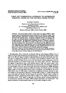
N (th) 1  exp(2t ) (36) 2 Let us study the impact of the two model parameters on the evolution of the mean number of preference particles. n(t ) 

The top panel of Figure 1 illustrates the impact of the coupling parameter. When the coupling parameter is increased, then the approach to the stationary value happens faster. The bottom panel of Figure 1 illustrates the impact of the volatility of the society. If the society is more volatile, then the stationary value is shifted to higher values.

100  

www.ccsenet.org/ijps

International Journal of Psychological Studies

Vol. 6, No. 4; 2014

Figure 1. Impact of the coupling parameter gamma (top panel) and volatility (bottom) Top panel parameters: N(th)=2.0, gamma was varied from 0.1 to 1 (bottom to top). Bottom panel parameters: gamma was equal to 1; N(th) was varied from 2 to 11 (bottom to top). All graphs were computed from Equation (36). The analytically obtained graphs can alternatively be computed from numerical simulations. This is illustrated in Figure 2. The dashed line in Figure 2 shows the analytical function. In contrast the solid line show the graph obtained from numerical simulation of a set of 100 trajectories. We found that the numerical result approximates to some extent the analytical function. Since the graph obtained by numerical simulations was calculated from a finite number (100) of agent trajectories, the numerically obtained result fluctuates and does not correspond to a smooth function. However, if the number of agents is increased then the numerically obtained graph becomes closer and closer to the analytically obtain function (data not shown).

Figure 2. Stochastic simulation (solid line) versus analytical result of the deterministic model (dashed line) The latter was computed from Equation (36) just as in Figure 1. Parameters: N(th)=2, gamma was equal to 1. The stochastic simulation of Equation (30) was conducted by means of an Euler-forward scheme with single time step 0.001 (Frank, 2005; Risken, 1989). The graph (solid line) shows the average of a total of 100 repetitions. Note that so far we did not take the decision making step into consideration. That is, the considerations presented above just address the increase of the number of preference particles and do not account for the fact that if for an individual agent the number reaches a critical threshold then a decision is made and the decision making process is terminated. Let us address next this decision making event. To this end, we consider the mean decision time of an ensemble of agents. This mean decision time is given by the so-called mean first passage time (MFPT) to reach the 101  

www.ccsenet.org/ijps

International Journal of Psychological Studies

Vol. 6, No. 4; 2014

threshold. That is, the mean decision time is the time on average it takes for the preference level to reach the threshold. Mathematically speaking, we have

1 R ( j) T  R  R j 1

TMFPT  lim

(37)

with

n ( j ) (t  T ( j ) )  

(38)

The mean decision time can be computed numerically using a large but finite set of agent trajectories. That is, in the numerical simulations R is finite. Before we present the results of such simulations, let us arrive at a hypothesis that can be tested in such computer experiments. As illustrated in Figure 1, an increase of the coupling parameter gamma yields a faster increase of the mean number of preference particles. Therefore, we speculate that the mean decision time as measured in terms of the MFPT becomes shorter when the coupling strength is increased. In order to test this hypothesis the mean decision time was computed for three values of coupling parameters gamma. The results are reported in Table 1. As expected, we found that the mean decision time decayed monotonically with increasing coupling strength. Hypothesis testing (ANOVA) showed that there was a statistical significant effect of the coupling strength on the mean decision time, F(2,27)=229.52, p