Mar 9, 2012 - model on a quasi-1-dimensional ladder filled with stationary anyons. .... The tunneling matrix between the legs at each rung corresponds to the coin shuffling ..... In the previous section, we derived the exact superoperator that ...
Quantum Walks of SU(2)k Anyons on a Ladder Lauri Lehman and Gavin K. Brennen Centre for Engineered Quantum Systems (EQuS), Macquarie University, Sydney, NSW 2109, Australia
Demosthenes Ellinas
arXiv:1203.1999v1 [quant-ph] 9 Mar 2012
Technical University of Crete, Department of Sciences, MΦQ Research Unit, GR-731 00 Chania, Crete Greece We study the effects of braiding interactions on single anyon dynamics using a quantum walk model on a quasi-1-dimensional ladder filled with stationary anyons. The model includes loss of information of the coin and nonlocal fusion degrees of freedom on every second time step, such that the entanglement between the position states and the exponentially growing auxiliary degrees of freedom is lost. The computational complexity of numerical calculations reduces drastically from the fully coherent anyonic quantum walk model, allowing for relatively long simulations for anyons which are spin−1/2 irreps of SU(2)k Chern-Simons theory. We find that for Abelian anyons, the walk retains the ballistic spreading velocity just like particles with trivial braiding statistics. For non-Abelian anyons, the numerical results indicate that the spreading velocity is linearly dependent on the number of time steps. By approximating the Kraus generators of the time evolution map by circulant matrices, it is shown that the spatial probability distribution for the k = 2 walk, corresponding to Ising model anyons, is equal to the classical unbiased random walk distribution.
I.
INTRODUCTION
Quantum walks have proven to be a fruitful model to study the dynamics of particles on lattices or more general graphs. The effects of exchange statistics on multiparticle quantum walks has been studied for bosons and fermions with a notable effect of statistics. For example it has been shown that quantum walks with non-interacting bosons give rise to effective interactions which lead to Bose-Einstein condensation in graphs with spatial dimension d < 2 [1]. Quantum walks with pairs of bosons or fermions have been studied in the context of the graph isomorphism problem by relating the Green’s function of the evolution to the spectrum of the graph. It was shown that these models have much more computational power when the particles are allowed to interact because they can distinguish non-isomorphic graphs that noninteracting particles cannot [2]. Recently using integrated photonics there has been experimental realization of two particle quantum walks which simulated bosonic, fermionic, and semionic (a type of Abelian anyon) statistics [3]. A natural extension of multiparticle quantum walks is to consider anyons which are particles that exist in two dimensions and have richer exchange statistics than bosons or fermions. In the case of Abelian anyons, exchanges, or braids, yield some model dependent phase eiφ while for non-Abelian anyons there is a large Hilbert space of fusion degrees of freedom of the multi particle system and a braid performs a unitary transformation on this vector space. A quasi-1-dimensional model for anyonic quantum walks was introduced in Ref. [4] where it was shown that Abelian anyons have quadratic variance just like standard quantum walks with trivial statistics but that non-Abelian anyons create entanglement during the walk purely due to braiding that acts to decohere the spatial degree of freedom. In Ref. [5] the quantum walk on a quasi-1-dimensional ladder was studied in detail for one type of non-Abelian anyon known as the Ising model anyon. This anyon corresponds to a spin−1/2 irrep. of SU (2)k=2 Chern-Simons theory, and the variance of the probability distribution of the walker was proven to be asymptotically linear in time with coefficient one, corresponding to the classical random walk behaviour. That particular case points out that there is a fundamental difference between the dynamics of Abelian vs. non-Abelian anyons. In this work we explore these differences for more general anyon models, specifically for spin−1/2 irreps of all values of the index k in SU (2)k Chern-Simons theory. Numerical results show that for small number of time steps, the position distribution approaches the quantum walk distribution as index k grows [4], and it was conjectured that the distribution looks classical when k � t. The problem with the fully coherent anyonic quantum walk is that to evaluate the probability distribution for t iterations of the discrete evolution operator, the number of paths which contribute to the walk grows exponentially with t. It turns out that evaluating each path is equivalent to computing the Jones polynomial for the link corresponding to the closed world line of that path, a computation which is itself exponentially hard (except for the cases k = 1, 2, 4 [6]) in the number of time steps t. To simplify the calculations for general k, we adopt here a special quantum walk protocol which introduces loss of memory to the coin and fusion degrees of freedom. Such a protocol allows for calculating the walk distribution for a relatively large number of time steps and to use certain approximations to diagonalize the walk operator and obtain analytical results.
2 II.
ANYONIC V 2 QUANTUM WALK
The anyonic quantum walk is a dynamical model for a single anyon (mobile or “walker” anyon) moving in a lattice of fixed anyons (stationary “background” anyons). The mobile anyon has an extra degree of freedom called the coin which is coupled to the direction of its movement. Here we consider a quasi-1-dimensional lattice of background anyons where the walker has only two directions of movement, left or right, and the coin is thus two-dimensional. Although the anyons are arranged on a line, they exist on a two-dimensional manifold such that the mobile anyon can pass them from above or below without coming into contact with the stationary This dynamics is accomodated � anyons. � by a walk on a ladder where the top(bottom) leg corresponds to mode 0 ( 1 ) of the coin, the sites correspond to the rungs and are labelled by an integer s, the stationary anyons are pinned in the islands of the ladder (see Fig. 1).
bs
0
UF s -1
s
s +1
s +2
1
FIG. 1: The anyonic quantum walk on a ladder of point contacts. The red oval is the walker anyon which moves along the black lines, and the grey ovals � are the stationary anyons which occupy the islands between the point contacts. The anyons are initialized in the state Φ0 meaning they are created out of the vacuum in pairs as indicated by the ovals joined by strings, and half of each pair is outside the ladder not participating in the walk. When on the upper(lower) edge the walker always to the left(right). The occupation sites of the mobile anyon are labelled by the positions s of the point contacts where the mobile anyon can tunnel. The tunneling matrix between the legs at each rung corresponds to the coin shuffling operator UF . Each lattice shift corresponds to a braid between the worldlines of the walker anyon and a stationary anyon, represented by the generator bs .
The arrangement in Fig. 1 is a crude model of quasiparticle dynamics in Fractional Quantum Hall samples which support anyonic quasiparticle excitations [7, 8]. The edge modes (horizontal in Fig. 1) carry mobile quasiparticles with a current direction determined by an externally applied voltage, and bulk quasiparticles can be pinned at antidots within the islands. The upper and lower edge modes are mixed by introducing point contacts controlled by front gates between the islands, allowing tunneling from edge to edge. The coin is thus encoded as propagation to left or right on the upper or lower edges respectively, and the scattering matrix that describes the tunneling between the edges represents the quantum coin flip operator. The model assumes a hardcore approximation for the anyons, such that they are always far apart, no polarization to fusion channels occurs and the anyons interact only non-locally via their braiding statistics. The model is also chiral: the particles on the upper edge are only allowed to move left and on the lower edge only to the right, and all braids are therefore anti-clockwise. When the walker shifts between lattice sites, the wave function is multiplied by the braid generator that corresponds to braiding the walker and the stationary anyon. The total Hilbert space is the tensor product space of the spatial � � N −1 sites, fusion degrees of freedom and the coin, H = Hspace ⊗Hfusion ⊗Hcoin . The position space is spanned by s s=0 , the fusion space accommodates 2N anyons (N − 1 stationary � anyons, � � the walker anyon and their antiparticle pairs) with total charge vacuum, and the coin space is spanned by 0 , 1 . We assume periodic boundary conditions, and choose the number of sites to be �
always larger than the length of the walk, N ≥ 4t + 1. The walker starts initially from the localized state s0 s0 . For reasons described below, rather than fully coherently evolving the system over many steps, the walk evolves coherently for two cycles followed over fusion and� coin � by tracing degrees of freedom. Afterward the fusion state is reset to the vacuum pair state Φ0 Φ0 , the coin state to c0 c0 , and the dynamics is iterated: � � �2 �† � ρS (t + 1) = Trf,c US UF ρS (t) ⊗ Φ0 Φ0 ⊗ c0 c0 (US UF )2 (1) UF = Ispace ⊗ Ifusion ⊗ H 1 H=√ 2
� � 1 1 1 −1
(2)
(3)
3 US =
N −1 � X
− Ss+1 ⊗ bs ⊗ P0 + Ss+ ⊗ bs ⊗ P1
�
(4)
s=0
� � − + when the Hadamard matrix � as the coin flip operator, Ss = s − 1 s and Ss = s + 1 s are the shift � H is chosen operators and P0 = 0 0 , P1 = 1 1 are projectors to the coin states. The braid generators bs are the matrices associated with braiding the anyons s and s + 1 in anticlockwise direction. Due to the periodic boundary conditions, there is also a braid generator bN −1 associated with braiding the anyons 1 and N which can be expressed in terms of the other generators1 , but we choose the system sizeQso that the walker never crosses the boundary and this generator is never applied. A string of braid generators, B = sj bsj is called a braid word. The braid matrices are determined by the anyon model in question. In a physical setting, the properties of the underlying material supporting the anyonic excitations determine the anyon model. We consider a general class of non-Abelian anyons corresponding to spin−1/2 irreps of the quantum group SU(2)k which is a group with a deformed version of the SU(2) algebra. The fusion rules of the SU(2)k model satisfy the triangle inequality and integer sum condition as in SU(2): j1 × j2 =
jX 1 +j2
j
j=|j1 −j2 |
but with two restrictions on the total spin charge j: j ≤ k/2;
j1 + j2 + j ≤ k
where j1 and j2 are two individual charges and the parameter k is the level of the theory. The Hilbert space of SU(2)k π ) is the quantum dimension. Since the fusion space grows anyons grows as dim(Hfusion ) ∝ dN where d = 2 cos( k+2 exponentially in the total number of anyons, if one is keeping track of correlations of the walker with the other anyons, the number of degrees of freedom to keep track of grows very fast with the number of time steps and the calculations become inefficient. To calculate the probability distribution of the walker for a given time step, only the calculation of the trace over the fusion degrees of freedom Fortunately, there exists a connection between the trace over �
is necessary. the representations of the braid group Φ0 B Φ0 and link invariants from knot theory that simplifies calculations of the trace. The trace over the fusion degrees of freedom can be understood in two equivalent ways: the usual matrix trace over the bracket representation of the density matrix of the fusion state, or the diagrammatic quantum trace which is defined by taking the fusion diagram representation of the state and joining the open ends of the incoming and outgoing charge indices [9]. The choice of which indices are joined together determines a tracing scheme for the braid word, and the tracing corresponds to a closure of a braid in knot theory, such that the closed braid forms a link. The usual tracing schemes are plat tracing, where the neighbouring charges are fused such that their total charge is vacuum, and Markov tracing, where each charge � is connected to itself before and after time evolution. We choose the initial state of the anyons Φ0 Φ0 such that the tracing corresponds to Markov tracing. The anyons are initially created from vacuum pairs, after which one member of each pair is dragged out of the system. In a braid presentation, this corresponds to having nearest-neighbour pairs with total charge vacuum, followed by a braid word which moves all left members of the pairs to the left. The total number of background anyons in an N -site walk is N − 1, but the total Hilbert space accommodates 2N anyons (background anyons, walker anyon, and their antiparticle pairs). Only half of the anyons participate in the quantum walk and after the two-step evolution are fused
all anyons � back together with their antiparticle pairs, see Fig. 2. In this scheme, the expectation value Φ0 B Φ0 corresponds diagrammatically to the Markov trace � over the braid word B.
� The virtue of using the state Φ0 as the initial fusion state is that the expectation value Φ0 B Φ0 can now be expressed in terms
� of the link invariant called the Kauffman bracket which is a Laurent polynomial in the variable A [10], denoted L (A), where L is a link, or a collection of tangled loops. This is written formally as
�
� L (A) Φ0 B Φ0 = n−1 (5) d � where L = (B Markov ) is the link obtained from the braid word B via closure by the initial state Φ0 , d is the quantum dimension of the anyons, n is the number of distinct components (strands) in the link L, and the value of
1
This generator can be explicitly written as bN −1 bN −2 . . . b2 b1 b†2 b†3 . . . b†N −2 b†N −1
4 4 8
6
2
1 3 5 7
=
3 1
5
2 4 6 8
B
7
FIG. 2: A link generated by the anyon worldlines in a quantum walk. Particle-antiparticle pairs are initially created from the vacuum state and one member of each pair is dragged out of the system. The walker anyon braids with the background anyons for two steps, after which each particle is fused back with their antiparticle pairs. Such a protocol implies that the diagrammatic tracing scheme is Markov.
the parameter for SU(2)k anyons is A = ie−iπ/2(k+2) . The calculation of the trace over the fusion states thus reduces to evaluation of the Kauffman bracket of the link that is drawn when the walker anyon moves on a particular path. The evaluation of the Kauffman bracket is not necessarily more efficient than calculating the matrix trace of the braid representations, but if one restricts to a model where the walker evolves coherently only for a finite amount of time steps, it turns out that for arbitrary long walks only a fixed number of links needs to be evaluated and the quantum walk distribution can be calculated exactly for fairly large number of time steps. In the usual quantum walk protocol, the quantum speedup occurs because the position of the walker becomes entangled with the coin. The system evolves coherently and the correlations between the position states and coin states preserve the memory in the system, hence the system dynamics is highly non-Markovian. If the walk is subject to decoherence, the correlations between the position and the coin become degraded and some of the memory in the system is lost. The loss of memory can be modeled using the so called “V n model” [11], where the state of the coin is erased and reset on every nth step, for example by doing a measurement on the coin and preparing it over again in the initial state. After resetting the coin, the system is in a product state and the correlations between the position and coin are lost. Remarkably even in the V 2 model there is enough coherence left in the system to provide for quadratic speed up over the classical random walk. Specifically, it was shown in Ref. [12] that the variance asymptotically scales like σ(t)2 = K2 t2 + K3 t for some constants K2 , K3 . Here the dynamics of our anyonic walk, Eq. 1, is the V 2 model where V = US UF . We write the dynamics as a super operator on the density operator ρs (t) for the spatial degrees of freedom of the walker: ρs (t + 1) = E(ρs (t)) =
Ph
� ��i � � h �† �2 i
� ρs (t) ⊗ Φ0 Φ0 ⊗ c0 c0 (US UF )2 I ⊗ f ⊗ c I ⊗ f ⊗ c US UF
f,c
=
Ph
� ��i
� �2 I ⊗ f ⊗ c US UF I ⊗ Ψ0 ⊗ c0 ρs (t)
f,c
h
≡
� ��i
� �† I ⊗ Φ0 ⊗ c0 (US UF )2 I ⊗ f ⊗ c
P f,c
Ef c ρs (t) Ef† c
where the Kraus generators have been defined as � ��
� �2 Ef c = I ⊗ f ⊗ c US UF I ⊗ Ψ0 ⊗ c0 .
(6)
Using equations (1)–(4) we find for the double step operator (US UF )2 =
NP −1 � s=0
� � s − 2 s ⊗ bs−2 bs−1 ⊗ P0 HP0 H + s s ⊗ b2s ⊗ P0 HP1 H
� � � + s s ⊗ b2s−1 ⊗ P1 HP0 H + s + 2 s ⊗ bs+1 bs ⊗ P1 HP1 H .
(7)
5 It is clear from this equation that the double step operator shifts the coefficients of the density matrix by two rows or columns, or not at all. By inserting this expression to and using the �
� the completeness � superoperator P P � † � of the fusion and coin bases, f bs Φ0 Φ0 bs0 f = Φ0 b†s0 bs Φ0 and c Pa HPb H c0 c0 H † Pa0 H † Pb0 c = c � f �
δa,b0 c0 H † Pa0 H † Pa HPb H c0 , the action of the superoperator on a general element s s0 of the spatial density matrix can be written as a sum of 7 terms: h � � � �
� E( s s0 ) = 41 s − 2 s0 − 2 Φ0 b†s0 −1 b†s0 −2 bs−2 bs−1 Φ0 + s − 2 s0 Φ0 b†2 s0 bs−2 bs−1 Φ0 �
� � � �
†2 2 �� 2 + s s0 − 2 Φ0 b†s0 −1 b†s0 −2 b2s Φ0 + s s0 Φ0 b†2 s0 bs Φ0 + Φ0 bs0 −1 bs−1 Φ0 (8) �
− s s0 + 2 Φ0 b†0 b†0 s
2 s +1 bs−1 Φ0
�
� � − s + 2 s0 Φ0 b†2 s0 −1 bs+1 bs Φ0
�i �
− s + 2 s0 + 2 Φ0 b†s0 b†s0 +1 bs+1 bs Φ0 . � � �
where we have chosen c0 = 0 such that c0 H † Pa0 H † Pa HPb H c0 = ± 41 . Equation (8) shows that for any element of the initial spatial density matrix, there are only seven nonzero elements of the superoperator E.� Writing the density matrix in a vectorized form, the superoperator can be written as a matrix: � P P ρ ~ 0 = f,c Ef c ⊗ Ef† c ρ ~, where the superoperator matrix f,c Ef c ⊗ Ef† c is a band matrix with seven diagonal � bands, and the rest of the elements are zero. Starting from the initial position density matrix ρs (0) = s0 s0 , the position density matrix after t time steps is obtained by applying the superoperator t times: � ρs (t) = E t ρs (0) . (9) �
† The elements of the are given by the product of the coin term c0 H Pa0 H † Pa HPb H c0 = ± 14 and superoperator � 0 the fusion term Φ�
0 B(s, s ) Φ0 . The probability distribution at time step t is obtained by starting from an initially localized state s0 s0 and applying the superoperator t times. The site probabilities are then given by the diagonal elements of the spatial density matrix. We have calculated the variance, σ(t)2 = hs2 i − hsi2 , of the V 2 walk for various choices of the level k up to t = 100 iterations of the superoperator, corresponding to 200 quantum walk steps. One interesting feature of the V 2 anyonic walk is that the effect of braiding statistics is trivial for Abelian anyons. If all the stationary anyons are of the same type, the walker always picks the same phase eiφ/2 when braiding with them, such that
� Φ0 B Φ0 = e−iφ/2 e−iφ/2 eiφ/2 eiφ/2 = 1. (10) This is similar to the fully coherent anyonic quantum walk, where the wave function always picks the phase eiφt/2 during the forward time evolution and phase e−iφt/2 during backward time evolution, such that the overall effect is trivial. Another way to think about the Abelian walk is to look at the case k = 1 in Chern-Simons theory. There are only two charges {0, 12 } in this model, the fusion channels are unambiguous: j1 × j2 = j, and the quantum dimension −iπ/6 is d = 1, so this model to the values of the brackets in Table I in Appendix A � is Abelian. Substituting A = ie 0 gives Φ0 B(s, s ) Φ0 = 1 for all brackets, confirming that the Abelian walk gives the same dynamics as the original V 2 quantum walk. The variance of the V 2 walk for Abelian anyons is plotted in Fig. 3 a). It shows the known fact [11] that the original V 2 walk propagates slower than the fully coherent quantum walk, but qualitatively the behaviour is still the same: the variance depends quadratically on time. The best fit for the variance of the k = 1 walk is given by σ 2 = 0.125 t2 + 0.75 t. In the non-Abelian case, the construction of the superoperator E requires evaluation of all eight expectation values in Eq. (8) for all s and s0 . The evaluation can be done by using the relation between the expectation values and the Kauffman bracket in Eq. (5). Each braid word consists of four braid generators, so that each planar representation of the corresponding link has four crossings. A very convenient feature of the link diagrams is that if s and s0 are far apart, the forward and backward braid words act on disjoint sets of strands, and the Kauffman brackets of all disjoint braids are equal (see Fig. 4 in Appendix A). Thus, the calculation of each expectation value involves only calculating the disjoint case and a small number of cases where s0 is close to s. The values of the expectation values are tabulated in Appendix A for all unique choices of s0 − s. The variances for various choices of k are plotted in Fig. 3 b). We observe that for k = 2, the variance follows exactly the linear line σ 2 = t. It is interesting to note that this behaviour is exactly the same as was shown for the fully coherent walk with k = 2 [5]. For the rest of the values of k, there is surprisingly small difference in the variance, with the slope of the variance slightly increasing as a function of k. For k = 3 and k = 4 (not shown in the figure) we
9000 8000 7000 6000 5000 4000 3000 2000 1000 0
220
k=1 RW QW
200 180 σ2
σ2
6
k=2 k=10 k->inf t
160 140 120 100
0
50
a)
100 Time step
150
200
100 b)
120
140 160 Time step
180
200
FIG. 3: The variance σ 2 of the two-step walk as a function of time t for various anyon models indexed by k. The scaling of the sites and time steps is chosen such that one iteration of the superoperator E corresponds to two iterations of the quantum walk time evolution operator, and at each iteration of E the walker shifts twice. a) Case k = 1 corresponds to the Abelian walk, which also coincides with the original V 2 quantum walk. Plotted for comparison are the variance of the classical random walk (RW) and the ordinary quantum walk (QW) with the same initial coin state and coin flip matrix. b) Non-Abelian SU(2)k models zoomed to the last 100 time steps. Also plotted is the linear curve σ 2 = t which corresponds to the classical random walk.
find that the slope of the variance is slightly smaller than 1, k = 3 having the smallest slope (best fit 0.9877). The highest variance is obtained when k → ∞, which corresponds to choice of the parameters A = i and d = 2, with slope 1.0665. It should be noted that in the fully coherent anyonic quantum walk model, taking the limit k → ∞ leads to the conventional SU(2) algebra, and the braiding generators are a non-Abelian representation of the permutation group. However when we introduced decoherence in the system, the braid words that contribute to the walk have different structure than in the fully coherent model. In the fully coherent model, the diagonal elements of the spatial degree of freedom of the walker correspond to a sum over all paths where the walker strand and necessarily all other strands return their initial position after forward and backward time evolution. Hence each of these paths is a trivial permutation in the fusion space and has no effect on the diagonal elements of the quantum walk. In the V 2 model however, the links do not have a dedicated walker strand as can be seen from Fig. 4 in Appendix A. The nontrivial character of the k → ∞ model thus follows from the fact that the links are not identity permutations and hence expectation values in Table I are not equal to 1, as they would be in the fully coherent walk. The key difference is that only for a highly non-Markovian environment does the k → ∞ case reduce to the normal quantum walk for only if one includes memory of all previous steps does the fusion DOF become disentangled with the spatial DOF.
III.
APPROXIMATION BY CIRCULANT MATRICES
In the previous section, we derived the exact superoperator that describes how the spatial density matrix transforms in a single step of the walk, and obtained numerical results by applying the superoperator to the density matrix repeatedly. We did not however obtain any expression for the density matrix after evolution by an arbitrary number of steps. In the following, we approximate the Kraus operators Ef c by circulant matrices which have uniform coefficients on each diagonal, and diagonalize the Kraus operators via Fourier transform to find arbitrary powers of the superoperator E in a compact form. Calling Eqs. (6) and (7) from previous section, the Kraus generators are written explicitly as Xh � �
� �
Cc00 f bs bs+1 Φ0 s s + 2 + f (Cc01 b2s + Cc10 b2s−1 ) Φ0 s s Ef c = s
�
� i + Cc11 f bs+1 bs Φ0 s + 2 s �
where the coin term has been defined as Ccab := c Pa HPb H c0 .
(11)
7 The matrix expression of the generators is df c (0) af c (0) ··· bf c (N − 2) d (1) a (1) bf c (N − 1) f c f c . . bf c (0) . df c (2) Ef c = . . .. .. bf c (1) af c (N − 3) . . .. .. af c (N − 2) ··· af c (N − 1) bf c (N − 3) df c (N − 1)
,
(12)
where �
af c (s) = Cc00 f bs bs+1 Φ0 , �
bf c (s) = Cc11 f bs+1 bs Φ0 , �
�
df c (s) = Cc01 f b2s Φ0 + Cc10 f b2s−1 Φ0 .
(13) (14) (15)
Comparing the matrix above with the general circulant matrix given in Eq. (B1) of the Appendix B, we see that although matrix Ef c is not a circulant matrix, it can be turned to a circulant matrix if the s-dependence of parameters af c (s), bf c (s), df c (s) is suppressed in some meaningful way, so that the sequences of these parametrers get approximated by some respective sequences e af c , ebf c and def c . This suppression of the s-dependence also leads to circulant form for Ef c . The advantage of having the Kraus generators being circulant matrices stems from the fact that the spectral decomposition problem of such matrices is solved (see Appendix B), and therefore this enables us to express the CP map of our QW and its powers in terms of the orthogonal eigenprojections of the generators. To this end we introduce for each af c (s), bf c (s) and df c (s) the following approximation for each s ∈ ZN 1 T r(b h2 Ef c ) N 1 df c (s) ≈ def c (s) = T r(Ef c ) N 1 bf c (s) ≈ ebf c (s) = T r(b h−2 Ef c ) N �
P where the elementary band matrices are defined as b h = s∈ZN s s + 1 . This is explicitly written as af c (s) ≈ e af c (s) =
e af c =
� Cc00 X f bs bs+1 Φ0 , N s
(16) (17) (18)
(19)
C 01 X 2 � Cc10 X 2 � def c = c f b s Φ0 + f bs−1 Φ0 N s N s
(20)
11 X � ebf c = Cc f bs+1 bs Φ0 , N s
(21)
i.e. the parameters af c (s), bf c (s), df c (s) are approximated by the arithmetic averages of the corresponding (f, Φ0 )elements of the respective generators. Denote Efwc the matrices obtained from Ef c by substituting the s-dependent terms with their averages: X �
X � X � s s + 2 + def c s s + ebf c s + 2 s Efwc = e af c (22) s
s
= e af c b h2 + def c Ib + ebf c b h−2 .
s
(23)
The map given by the new Kraus generators Efwc is not trace preserving, so we are seeking for a set of generators ef c which satisfy the trace preserving condition P E e† e E f,c f c Ef c = I. To this end we need to scale the circulant P w† w e matrices Efwc by f c Ef c Ef c ≡ M , so the new trace preserving circulant Kraus generators are defined Ef c = P w −1/2 ( f,c Efw† Efwc ≡ Λ Efwc with Λ = M −1/2 . c Ef c ) A calculation gives M = κ1 I + κ2 b h2 + κ∗2 b h−2
(24)
8 where � |e af c |2 + |def c |2 + |ebf c |2 f,c � � P = 14 N12 j,j 0 Φ0 b†j 0 +1 b†j 0 bj bj+1 Φ0 +
κ1 =
κ2 =
P
1 4
�
1 N2
P
j,j 0
� Φ0 b†j 0 b†j 0 +1 b2j−1 Φ0 +
2 N2
1 N2
P
j,j 0
P
j,j 0
†2 2 � Φ 0 b j 0 b j Φ0 +
Φ0 b†2 j 0 bj bj+1 Φ0
1 N2
��
P
j,j 0
�� Φ0 b†j 0 b†j 0 +1 bj+1 bj Φ0
(25)
.
The matrix M is a circulant band matrix which can be diagonalized via discrete Fourier transform F (see Appendix B): X � � F †M F = κ1 + κ2 ω 2l + κ∗2 ω −2l l l . l
The matrix F † M F is a diagonal matrix with all diagonal values nonzero, so its inverse exists. The normalization �−1/2 � P l l . operator Λ can now be defined as Λ = F (F † M F )−1/2 F † , where (F † M F )−1/2 = l κ1 + κ2 ω 2l + κ∗2 ω −2l 2 −1/2 A simple check verifies that Λ M = I and Λ = M as desired. ˆ for general values ef c = ΛEf c contain all even powers of the matrices h Unfortunately, the normalized generators E of the Chern-Simons parameter k and do not admit a helpful form. However, for the special values k = 2, 4 there is a significant simplification. Notice that each of the terms in expressions for κ1 , κ2 in Eq. (25) is an averaged Kauffman bracket. For large N most of these brackets will correspond to disjoint links, i.e. the links formed by two step walks involving the strands located at j and j 0 do not entangle. As shown in Table I, this always occurs if |j 0 − j| > 3. If we approximate the average by the value of the bracket for these disjoint links then κ1 =
1 32
κ2 =
1 8
�
� 2π 4π 6π π 6 cos( k+2 ) + 4 cos( k+2 ) + 2 cos( k+2 ) + 5 sec4 ( k+2 ) + O(1/N ) (26)
�
4π cos( k+2 )
−
2π cos( k+2 )
�
+ 1 sec
2
�
π ( k+2 )
+ O(1/N ).
where the error is of order 1/N . Thus at the special values k = 2, 4 we have κ2 ≈ 0 and the normalization operator −1/2 becomes a scalar multiple of the identity: Λ = κ1 I. Henceforth we focus on the case k = 2 since the behaviour of k = 4 is quite similar. The Kraus generators are given by � ef c = κ−1/2 e E af c b h2 + def c Ib + ebf c b h−2 . 1
(27)
� P The elementary circular matrix b h can now be diagonalized as F † b hF = gb = n∈ZN ω n n n where ω = e2πi/N . This allows to write the Kraus generators in a diagonal form � ef c = κ−1/2 F e E af c gb2 + def c I + ebf c gb−2 F † 1 X ≡ λf c (k)Pfk
(28) (29)
k∈ZN
� � −1/2 with λf c (k) = κ1 e af c ω 2k + def c + ebf c ω −2k and Pfk = F k k F † . The action of the superoperator Ee on a spatial density matrix ρS is then given by X X X e S) = ef c ρS E e† = E(ρ E λf c (k)λ∗f c (l)Pfk ρS Pf†l (30) fc f,c
f,c k,l∈ZN
and for t time steps Eet (ρS ) =
t X X Y
� λfi ci (k)λ∗fi ci (l) Pfk ρS Pf†l .
(31)
k,l∈ZN i=1 fi ,ci
Let’s use this compact form to calculate the diagonal probability distribution p(s, t) at time t: p(s, t) = � �
t s Ee (ρS (0)) s . Let’s assume that the walker is initialized in the position eigenstate s0 , that the size of the
9 � periodic lattice is N , and that during the 2-step walk the coin is always reinitialized to state c = 0 . We find for the index k = 2: pIsing (s, t) = hs|Eet (|s P0 ihs0 |)|si = 2t 1N 2 r,l∈ZN ω (s−s0 )(r−l) (ω 2(r−l) + ω −2(r−l) )t � Pt t P ω (s−s0 )(r−l) ω 2m(r−l) ω −2(t−m)(r−l) = 2t 1N 2 m=0 m � r,l∈ZN r(s−s +4m−2t) P P t t P 1 −l(s−s0 +4m−2t) 0 = 2t N 2 m=0 m ω l∈ZN ω � r∈ZN Pt t 1 2 = 2t N 2 m=0� m (N δs−s0 +4m−2t,0 ) t = 21t 2t−(s−s 0)
(32)
4
This is the binomial distribution where the range of the sites is s ∈ [−2t, 2t] and the probabilities are nonzero only for s = s0 + 4n, n ∈ Z, i.e. the V 2 model with k = 2. Ising anyon walkers therefore have the same probability distribution as the classical random walk where every step moves two units to the right or left and the variance, scaled so that 2 each two steps move takes place over two time intervals, is σIsing (t) = t. IV.
CONCLUSIONS
We have considered a lossy anyonic quantum walk protocol where the entanglement between the spatial modes of the walker and its environment, the coin and fusion space, is lost on every second step. We calculated the time evolution of the exact probability distributions for various values of the parameter k in Chern-Simons theory. The case k = 1 corresponds to the Abelian anyonic quantum walk and it was found to be equal to the standard V 2 quantum walk with trivial exchange statistics, the variance of which has a leading term proportional to t2 . Cases k ≥ 2 are non-Abelian anyon models, for which the variance grows linearly as a function of time for all tested values of k in the time scales of up to 100 iterations of the superoperator. By approximating the Kraus generators of the superoperator by circulant matrices, the generators can be diagonalized for k = 2, 4. This allows for a compact expression for the probability distribution after arbitrary number of iterations of the superoperator. The expression for k = 2 is the binomial distribution which is equal to the classical random walk distribution. Thus the V 2 anyonic quantum walk with Ising anyons has the same behaviour as the fully coherent walk, which was also shown to have a linear variance with coefficient 1 [5]. In the fully coherent walk, the slowdown of the walker propagation can be explained by decoherence: the fusion Hilbert space of non-Abelian anyons acts like an environment to the walker+coin system, degrading the quantum correlations between the spatial and coin modes which are the origin of the quantum speedup. It was conjectured in Ref. [5] that the slowdown happens when the parameter k is much smaller than the number of time steps t, k � t, ie. for any finite k, the walk behaves classically in the large time limit. In the V 2 model presented here the results support that conjecture. There are two kinds of decoherence mechanisms at work, one due to the fusion space of the anyons and the other because the entanglement between the spatial modes and the coin is lost. The loss of quantum correlations on every second step does not change the qualitative behaviour when the braiding statistics is Abelian, but when the additional effect of the fusion space comes into play for non-Abelian anyons, the spreading velocity changes to diffusive for all values of k for long enough times (in fact after fewer than 100 steps). The V 2 model can be easily generalized to V n models where the walk evolves coherently for n time steps instead of two. Evaluation of higher number of time steps becomes increasingly hard, because the number of different Kauffman brackets that need to be computed increases as the walker is allowed to do more steps between the tracing operation. One might expect that for large n, the walker propagates diffusively for n steps for small k and ballistically for large k, before the tracing is carried out. However, as we have shown, the variance of the anyonic V 2 walk is linear even when k � 2, so we expect that in the long time limit the variance is linear for all V n models, although the walker might spread ballistically in the initial stage of the walk. It is known that spatial randomness in the coin operator can lead to localization of the walker wave packet [13], ie. the probability to stay in the initial position becomes very high and the probability falls off exponentially away from the initial position. In the anyonic quantum walk setup, spatial randomness can also occur if the occupation numbers of the background anyons fluctuate randomly. These fluctuations might occur when thermal excitations create particleantiparticle pairs from vacuum, for example. It is interesting to note that if the occupation numbers of the islands are not uniform, the Abelian anyons can pick up different phases during forward and backward time evolution, and the effect of the braiding statistics becomes nontrivial. We have calculated evolution of the V 2 anyonic walk with random fillings of Abelian anyons on the islands, but observed diffusive spreading (no localization). Localization is a quantum phenomenon that requires interference of the probability amplitudes to occur. Interestingly our results show that while the memory loss in the V 2 model preserves enough coherence in the Abelian walk to provide for quadratic
10 speed up without disorder, it does not provide enough to give localization with disorder. Rather the competition of the two effects yields classical behaviour. Acknowledgements
One of us (D.E.) is grateful to the Department of Physics and Astronomy, Macquarie University for hospitality during a sabbatical stay during which this work was initiated. Appendix A: Braid group matrix elements
The construction of the superoperator E requires calculating the eight expectation values in Eq. (8) for all values 0 of
�s and s . The expectation values are related to the Kauffman bracket via Eq. (5). Kauffman bracket polynomial L (A) in the variable A [10] is a link invariant for framed, unoriented links. The defining properties of the Kauffman bracket are given by the uncrossing relation and two relations for removing loops from the bracket: D E D E D E =A + A−1 (A1)
�
� L ∪ = −(A2 + A−2 ) L
(A2)
�
= 1.
(A3)
The value of the Kauffman bracket for a specific braid word can be calculated by forming the link diagram that corresponds to the braid presentation and Markov closure of the word. The unique link diagrams for one braid word are drawn for illustration in Fig. 4. The value of the bracket polynomial is then obtained by applying the relations (A1) and (A2) to the link diagram, removing all crossings and loops in the diagram except one. The bracket of a single loop is trivial, so the remaining coefficient is the value of the bracket polynomial.
s-1
s
s'
s'+1
s-1
s'+1
bs' bs'+1 bs-1 bs-1 a)
b)
�
FIG. 4: Two links corresponding to the expectation value Φ0 b†s0 b†s0 +1 b2s−1 Φ0 . a) Case s0 − s = 1. The forward braids b2s−1 and the backward braids b†s0 b†s0 +1 act on separate sets of strands, therefore the links corresponding to the forward and backward braids are disjoint. The links corresponding to s0 − s ≤ −4, s0 − s ≥ 1 are all disjoint and the values of the Kauffman brackets are the same. b) Case s0 − s = −1. The forward and backward braids now form a joint link.
For SU(2)k anyons, the value of the parameter is A = ie−iπ/2(k+2) , and the quantum dimension satisfies d = π ). For s0 − s large, the forward and backward braid words never touch the same strands, the −(A2 + A−2 ) = 2 cos( k+2 links corresponding to forward and back evolution are disjoint, and value of �the Kauffman bracket polynomial is
the equal for all s and s0 . Thus, the calculation of a general element Φ0 B(s, s0 ) Φ0 involves only the calculation of the disjoint element and a few cases where s0 − s is small. The unique values of five of the expectation values are given in Table I. For the remaining elements, we have
†2 2 � †2 2 � Φ0 bs0 −1 bs−1 Φ0 = Φ0 bs0 bs Φ0
11 � � Φ0 b†s0 −1 b†s0 −2 bs−2 bs−1 Φ0 Φ0 b†s0 b†s0 +1 bs+1 bs Φ0
s0 − s
−2 −1 0 1 2 ≤ −3, ≥ 3
d−4 d−2 1 d−2 d−4 d−4
d−4 d−2 1 d−2 d−4 d−4 � † † � Φ0 b†2 Φ0 bs0 bs0 +1 b2s−1 Φ0 s0 bs−2 bs−1 Φ0
s0 − s
−3 −2 −1 0 ≤ −4, ≥ 1
−A6 (A4 + A−4 )/d3 d−2 d−2 −A6 (A4 + A−4 )/d3 −A6 (A4 + A−4 )/d3
−A−6 (A4 + A−4 )/d3 d−2 d−2 −A−6 (A4 + A−4 )/d3 −A−6 (A4 + A−4 )/d3
� 2 Φ0 b†2 s0 bs Φ0
s0 − s
−1 0 1 ≤ −2, ≥ 2
(A4 + A−4 )2 /d2 1 (A4 + A−4 )2 /d2 (A4 + A−4 )2 /d2
TABLE I: The values of the braid group elements involved in the evolution CP map.
and the conjugate transpose elements � ��∗
† Φ0 bs0 −1 b†s0 −2 b2s Φ0 = Φ0 b†2 s bs0 −2 bs0 −1 Φ0 and � ��∗
†2
Φ0 bs0 −1 bs+1 bs Φ0 = Φ0 b†s b†s+1 b2s0 −1 Φ0 .
Appendix B: Circulant matrices and CP map generators
A matrix C = (cij ) of order n is called a circulant matrix [14] if cij = ai−j( mod n) . The entries of the first column a ≡ (a0 , a1 , ..., an−1 ) determine the entire circulant matrix which we denote Cn = circ(a) = circ(a0 , a1 , ..., αn−1 ), and in matrix form it reads Cn =
a0 a1 a2 .. .
an−1 an−2 a0 an−1 a0 .. .. . .
an−1 an−2 an−3
· · · a1 · · · a2 · · · a3 . . . .. . . · · · a0
(B1)
�
P Alternatively circulant matrices are written in terms of elementary circulant matrix b h = m∈{0,1,...,n−1} m m + 1 = circ(0, 1, ..., 0), as Cn = circ(a0 , a1 , ..., αn−1 ) = p(b h) where p is the polynomial p(z) := a0 + a1 z + · · · an−1 z n−1 . Matrix b h is diagonalized by the finite Fourier transform unitary matrix F , with elements Fab = √1 ω ab , ω = n
i2π/n
†b
n−1
e , as F hF = gb, where gb = diag(1, ω, ..., ω ). Any circulant matrix is then canonically decomposed as Cn = circ(a0 , a1 , ..., αn−1 ) = F † diag(p(1), p(ω), ..., p(ω n−1 ))F. A banded circulant matrix is a circulant matrix
12 for which only a connected subset in the sequence a = (aj )n−1 After introducing the approxij=0 is non zero. mations issued in Eqs. (16)–(18) the generators Ef c of QW’s CP map become banded circulant matrices i.e. ef c = circ(a0 = def c , a1 = 0, a2 = ebf c , ..., an−2 = e E af c , an−1 = 0). P Circulant matrix b h = s∈ZN |si hs + 1| , and its inverse b h−1 0 1 1 0 X b , 1 0 h = |n + 1i hn| = .. n . 1 1 0 0 1 0 1 X −1 b , 0 1 h = |n − 1i hn| = .. n . 1 1 0
(B2)
(B3)
P generate the abelian group {b ha }a∈ZN ' ZN , share the property b h2 = 1. h† = b h−1 = s∈ZN |s + 1i hs| , where b An important tool used in Sec. III to approximate the V 2 quantum walk model is the optimal circulant of a matrix. For an arbitrary square matrix D = (djk ), i, k = 0, 1, ..., N − 1, we choose a suitable circulant matrix C. For the construction of C it has been recommended [15], (after preliminary transformations such as changing the order of the rows and multiplying them with suitable constants), to apply the following: by imposing periodicity i.e. dj+N,k = dj,k , PN −1 form the arithmetic averages of the elements along the diagonals i.e. aj = N1 k=0 dj+k,k , and construct in this way the circulant C = circ(a0 , a1 , ...maN −1 ). On the other hand an optimal circulant approximation of some Toeplitz matrix T (see e.g. Strang’s suggestion in [16]), have been constructed by determing the nearest circulant with respect to Frobenius matrix norm for matrix T , i.e. by solving the optimization problem minC:circulant kT − CkF [17]. The resulting circulant coincides with the one obtained by the method of arithmetic averages [15], applied to T . In the quantum walk context the method of ef c . arithmetic averages is been applied to the Kraus generators Ef c that are approximated by the optimal circulant E
[1] R. Burioni, D. Cassi, I. Meccoli, M. Rasetti, S. Regina, P. Sodano, and A. Vezzani, Europhys. Lett. 52, 251 (2000). [2] J.K. Gamble, M. Friesen, D. Zhou, R. Joynt, and S.N. Coppersmith, Phys. Rev. A 81, 052313 (2010). [3] L. Sansoni, F. Sciarrino, G. Vallone, P. Mataloni, A. Crespi, R. Ramponi, and R Osellame, Phys. Rev. Lett. 108, 010502 (2012). [4] G. Brennen, D. Ellinas, V. Kendon, J. Pachos, I. Tsohantjis and Z.Wang, Ann. Phys. 325, 664 (2010) [5] L. Lehman, V. Zatloukal, G. Brennen, J. Pachos and Z. Wang, Phys. Rev. Lett. 106, 230404 (2011). [6] F. Jaeger, D.L. Vertigan, and D.J.A. Welsh, Math. Proc. Camb. Phil. Soc. 108, 35 (1990). [7] R.L. Willett, L.N. Pfeiffer, and K.W. West, Proc. Nat. Acad. Sci. 106 8853 (2009). [8] P. Bonderson, K. Shtengel, and J. Slingerland, Ann. Phys. (N.Y.) 323, 2709 (2008). [9] P. Bonderson, PhD Thesis, California Institute of Technology (2007) [10] L. Kauffman, Topology 26, 395 (1987) [11] A.J. Bracken, D. Ellinas, and I. Tsohantjis, J. Phys. A 37, L91 (2004); [12] D. Ellinas and I. Smyrnakis, Physica A 365, 222 (2006). [13] E. Hamza et al, Math. Phys. Anal. Geom. 12, 381 (2009); N. Linden and J. Sharam, Phys. Rev. A 80, 052327 (2009); A, Joye and M. Merkli, J. Stat. Phys. 140, 1 (2010); A. Albrecht et al, J. Math. Phys. 52, 102201 [14] P. J. Davis, Circular Matrices, 2nd ed., Chelsea Publ. (New York 1994). [15] L. Berg, ZAMM - Journal of Applied Mathematics and Mechanics Zeitschrift fur Angewandte Mathematik und Mechanik 55, 439 (1975). [16] G. Strang, Stud. Appl. Math. 74 171 (1986) [17] T. Chan, SIAM J. Sci. Statist. Comput. 9 766 (1988)