Andrei Ludu and Walter Greiner. Institut für Theoretische Physik der. J. W. Goethe - Universität, Robert-Mayer-Strase 8-10, D-60054, Frankfurt am Main,.
Quasi-continuous symmetries of non-Lie type
arXiv:q-alg/9612004v1 2 Dec 1996
Andrei Ludu and Walter Greiner Institut f¨ ur Theoretische Physik der J. W. Goethe - Universit¨at, Robert-Mayer-Strase 8-10, D-60054, Frankfurt am Main, Germany
Abstract We introduce a smooth mapping of some discrete space-time symmetries into quasi-continuous ones. Such transformations are related with q-deformations of the dilations of the Euclidean space and with the non-commutative space. We work out two examples of Hamiltonian invariance under such symmetries. The Schr¨ odinger equation for a free particle is investigated in such a non-commutative plane and a connection with anyonic statistics is found.
.
PACS: 03.65.Fd, 11.30.Er
1
Continuous symmetries are generally described in terms of Lie groups and algebras through their irreducible unitary representations acting on the Hilbert space of states. Among these, the space-time symmetries are expressed as the invariance of the dynamical equations under transformations of the coordinate frame. One advantage of continuous symmetries over the discrete ones appears clearly in the Lagrangean field theories where, due to the Noether theorem, one can define currents and conserved quantities associated with the time evolution of the dynamical system. The discrete symmetries arising in physiscs can be clasificated in Z2 graded symmetries consisting in inversions of the space (parity P, reflexions, mirroring), charge conjugation (C) and time reversal (T) on one side, and permutations and braids on the other side. The former act on one-particle states or directly on the space-time manifold. The operators associated with these symmetries have the square equal with one. The latter ones act on many-particle states, and they are connected with the statistics of the physical system; they are finite or infinite dimensional unitary irreducible representations of some discrete groups over some Hilbert space of states. In this paper we introduce a continuous algebra of transformations in which are embedded some discrete space-time symmetries. A first direct way to construct such a structure is to introduce an associative continuous algebra of operators, defined by some commutator relations, containing the identity and the discrete transformations among its elements. Such an algebraic-continuous structure is more general then Lie algebras or loop groups. If both the identity and the discrete symmetries could be brought together in the same smooth algebraic structure, it is possible that new symmetries (associated with the intermediate steps in between the identity-discrete limits) could occure. We show in the following that such a structure exists and can be obtained as a q-deformed algebra. Quantum groups [1-3] (quantized universal enveloping algebras, q-algebras, q-deformations) have been the subject of numerous recent studies in mathematics and physics. They represent some special deformations (q 6= 1) of the universal enveloping algebra of Lie algebras (q = 1) [1-3]. For a recent review see [4]. In the present paper we are both interested in some limiting cases of the q-deformations, which should meet the discrete original symmetries, and in the intermediate (nongeometric) symmetries (joining the discrete elements). The mapping of the discrete symmetries on the continuous ones results in interesting consequences for the space-time discretisation, 2
non-commutative spaces and spontaneous breaking of symmetry. We introduce the R3 Euclidean (commutative) space generated by (xi ) = (x, y, z) and its tangent space, generated by ∂i = ∂/∂xi . Twelve infinitesimal (Lie) generators ξˆ ∈ {∂i , xj ∂i }, act on the product space of R3 with its tangent space. With these generators one constructs different Lie algebras with action on the functions defined on R3 . We associate to each generator ξˆ a one-real parameter Lie group, g(φ)|φ∈R by ˆ In order to play an example, we way of the exponential map ξˆ → g(φ) = exp(φξ). restrict to the following discrete transformations, acting on R2 : identity 1, infinitesimal generator of rotations in plane v (or finite rotation of −π/2), reflection against Oy axis ry and permutation P (or reflection against the line x = y). They satisfy the relations: ry2 = P 2 = 1, v 2 = −1, and (excepting I) they generate a Lie algebra, isomorphic with su(2), and defined by the commutators: [v, ry ] = 2P, [P, v] = 2ry , [P, ry ] = 2v.
(1)
The isolated (discrete symmetries) P and ry , can not be regarded as group elements, since they do not belong to any representation of SU(2), hence they are not realised in terms of a certain g(φ), for any φ. Consequently, following the Lie approach, one can not smootly map the identity group element into P or ry . In fact, this conclusion is the algebraic formulation of the geometric imposibility of continuously mapping the y axis into the −y axis through a Lie transformations (rotations against the x axis, dilation of the y axis, etc), in two dimensions only. All such methods always yield to intermediate situations having algebraic singularities: the number of dimensions increases to three or decreases to one. From the topological point of view the mirror transformation ry is similar with the problem of mirroring a knot [5]. The right-handed and the left-handed coordinate frames of the plane are actualy oriented knots since one of the axis always undercrosses the other. The coordinate frame is an oriented knot which holds the same topological informations as the original image. So, the discrete transformation ry of the coordinate frame, can be realised as a mirror transformation of a knot (the interchanging of the roles of undercrossed/overcrossed at each knot of a diagram). There are examples of (achiral) knots which can be continuously deformed into their mirror image (Eight knot) and examples of (chiral) knots which can not (Trifoil knot) [5]. This continuous deformation is a finite succesion of Reidemeister moves of ambiental 3
isotopy (transformations in the plane which simulate the corresponding natural topological transformations in the 3-dimensional space of the unfolded correspondent of the knot). Consequently, an algebraic treatment of the Reidemeister moves can direct the problem to the construction of a continuous connection of the discrete mirrorings with the identity. Since the quantum group glq (2) provides representations of such moves [5], we construct in the following special q-deformations of the Lie algebra gl(2) in relation with knots and braids. In order to use such deformations we introduce the q-deformed commutators in the form [x, y]q ≡ xy − qyx, [x, y]q=1 = [x, y], [4]. Such relations exist in the universal enveloping algebra of all the products of the generators, and they generate a special type of quantum group. By introducing the transformations. Ry = ry + v, V = ry − v we have the new commutators: [Ry , P ]q = (1 + q)Ry , [V, P ]q = −(1 + q)V, [Ry , V ]q = 2((1 − q)1 − (1 + q)P ).
(2)
We remark that in the last commutator we have obtained a deformed element which maps 1 into P , when q goes from q1 = −1 to q2 = 1. An example of action of the above defined deformed commutators on the real line is given by introducing a quantum analogue of the x coordinate through the operator ˆ xˆ = xQ(x∂ x , q),
(3)
ˆ x , q) is a linear operator given by a function of the infinitesimal generator of where Q(x∂ ˆ = 1. Following dilations x∂x and deppending on the parameter q, such that limq→1 Q [6,7] the corresponding canonical momentum is defined as ˆ ∂ˆx = Q(x∂ x , q)∂x .
(4)
From eqs.(3,4) it results the following commutation relation: [∂ˆx , xˆ] = 1 + (q 2 − 1)ˆ x∂ˆx ,
(5)
or, written in the formalism of q-deformed commutators, [∂ˆx , xˆ]q = 1.
4
(6)
Eq.(6) becomes the usual commutator relations between the x and ∂x operators, in the ˆ defined in eq.(4) must satisfy the condition limit q → 1. From eq.(6) the operator Q ˆ 2 + Qx∂ ˆ xQ ˆ = 1 + q 2 xQ ˆ 2 ∂x , Q which, applied on integer real functions f (x) =
P
j
(7)
fj xj , reads
ˆ 2 (j) = 1 + q 2 j Q ˆ 2 (j − 1), (j + 1)Q
(8)
From eq.(8) we obtain the solution ˆ 2 (j) = q j [j + 1] , Q j+1
(9)
where [j + 1] is the q-deformation of j + 1, [3,4]. Consequently, we have the realisation of the new coordinate operator in the form xˆ =
v u u xtq x∂x
q 2x∂x − 1 . (q − 1)(x∂x + 1)
(10)
similarly with the realisation introduced in [7]. In order to evoid the square root occuring in eq.(10) we can modify the q-deformed commutator relations, preserving the same behaviour in the limit q = 1. If the new coordinates of the phase-space satisfy ˆ
[∂ˆx , xˆ] = q 2ˆx∂x ,
(11)
ˆ a simpler form: by following the same procedure similar with eqs.(6,7) we get for Q ˆ = q x∂x , Q
(12)
which gives us just the dilation operator. In order to generalise the above construction we have to introduce a set of continuous transformations of the coordinates, depending on one complex parameter q, having no Lie algebraic equivalent and which, for certain fixed values of q, approache the space inversions Iˆx , Iˆy , Iˆz . These general structures are nonlocal, non-Lie and nonlinear transformations, i.e. they do not form a Lie group (they are not of the form eǫv with v a vector field of a Lie algebra not depending on ǫ). We introduce over R3 the infinitesimal generators of the dilation dˆi = xi ∂xi and ˆ k, D ˆ j ] = 0, ˆ k (s) = q dˆk = eisdˆk , [D their corresponding one-dimensional Lie groups D 5
where we use a complex deformation in the form q = eis with s ∈ [0, π]. The action of the dilation operators on analytical functions on R3 is continuous with respect to s. In ˆ i → 1 and in the limit q → −1 (s → π) we have the limit q → 1 (s → 0) we have D ˆ i → Iˆi . Consequently, in the range s : [0, π] the operators D ˆ i smoothly map the unit D
ˆ i (π) = Iˆi generating in this way element into the corresponding inversion operator Iˆi , D ˆ dˆi , s) = Pk Ck (s)dˆk all the inversions of R3 . A q-deformed operator integer function Q( i
ˆ s)xji ˆ dˆi, s)f (xi ) = j fj Q(j, Q( has the action on real integer functions f (xi ) = ˆ dˆi, 1) = 1. This operator should be linear and should which approaches f (xi ) for Q( ˆ dˆi , 1) = 1, Q( ˆ dˆi, −1) = eiπdˆi = Iˆi . have the following limits: Q( P
j j fj xi ,
P
In the following we we want to find the most general one-dimensional Hamiltonian having a symmetry for these types of transformations. In the one-dimensional case ˆ is invariant to the symmetry introduced by the operator (xi = x) a Hamiltonian H ˆ = Q( ˆ dˆi , s) if [H, ˆ Q] ˆ = 0. We choose a general one-dimensional Hamiltonian in the Q form ˆ = −∂ 2 + V (x) + W (x∂x ), H x
(13)
ˆ (x) = Ef (x). The Hamiltonian consists and the corresponding Schr¨odinger equation Hf Vj xj and an effective P ˆ potential W (x∂x ) = Wj (x∂x )j . The last term commutes with Q. ˆ under the transformation Q, ˆ [Q, ˆ H]f ˆ (x) = 0 The condition of symmetry of H
of the sum of the kinetic energy term, a local potential V (x) =
applied to an arbitrary integer function f (x) = responding powers of x, reads ˆ ˆ + 2)) = fk+2 (k + 1)(k + 2)(Q(k) − Q(k
P
P
j
fk xk , after identification of the cor-
k−1 X j=0
ˆ ˆ Vk−j fj (Q(k) − Q(j)).
(14)
Eq.(14) must be solved together with the Schr¨odinger equation for f which, expanded in powers of x, reads: fk+2 (k + 1)(k + 2) =
k X l=0
fl Vk−l − Efk + fk W (k).
(15)
ˆ=D ˆ x eq.(14) becomes In the simplest case Q fk+2 =
Pk−1
Vk−j fj (1 − q j−k ) . (1 − q 2 )(k + 1)(k + 2) j=0
6
(16)
Eqs.(14,15) give the conditions for the existence of the continuous symmetry described ˆ Both these equations are identities for Q ˆ = 1. In the case of the by the operator Q. ˆ → Iˆx , i.e. Q(k) ˆ inversion x → −x, Q = (−1)k , eq.(14) asks for Vk = fk = 0, for k odd, (V (−x) = V (x), f (x) = f (−x)) like in the traditional case. In the free particle case we have V (x) = 0 and from eq.(14) we get ˆ ˆ + 2), Q(k) = Q(k
(17)
ˆ odd ) = ±1 and Q(k ˆ even ) = 1. This restricts the allowed symmetries for the and Q(k free particle to inversion only. For any potential of the form V (x) = xn we obtain
the corresponding invariance condition q n = 1. In this case the number of admissible discrete symmetries between 1 and Iˆx is finite (n roots of the unity) and still there is no way of continuous mapping of the identity into the mirroring. ˆ = D. ˆ From eq.(14) we note We want to solve eqs.(14-15) in the simple case of Q that a full invariance of the wavefunction f (x) occures if the potential V (x) depends also on q. Hence, we introduce and arbitrary potential V 0 (x) =
P
k
Vk0 xk independent of q,
and we write the potential of the Hamiltonian in eq.(13) in the form of a transformation V (x) → V (x, q) =
X
Vk (q)xk =
k
1 X 0 q2 − 1 k x , kVk 2 k 1 − q −k
where the coefficients Vk0 (independent of q) determine the limit V (x, 1) =
(18) P
k
Vk0 xk =
V 0 (x). Due to this choice, eq.(14) does not depend any more on q and one can obtain the coefficients fk as function of Vk0 only. This procedure makes sense only if the coefficients 1 − q k−j in eq.(16) are not zero. This condition depends on j, k and consequently on the nonzero coefficients of V (x, q) in its Taylor expansion, and on the values of q. If we do not have such singularities (e.g. for s irrational multiples of π) the corresponding ˆ wavefunctions do not depend on q, i.e. do not depend on the global transformation Q, for any q, from the identity (q = 1) to the inversion (q = −1): fk+2 =
0 Vk−j fj . (k + 1)(k + 2)
P
k
(19)
ˆ ′s The physical system remains in the same quantum state under the action of all Q from ˆ1 to Iˆx . With the coefficients fk of the wavefunction obtained from eq.(19) we can determine the coefficients W (k) and E in eq.(15). Thus, we obtain a dynamical 7
ˆ symmetry for the Hamiltonian in eq.(13) under Q(x∂ x , q), with its eigenfunctions f (x) ˆ and eigenvalues E independent of q. As a consequence, the transformations Q(x∂ x , q) keep invariant the physical states. However the associated potential transforms with q, like in the case of a gauge transformation. The transformations of the potential, given by eq.(18), can be written explicitely in the form of a nonlocal operator applied on V 0 (x), for |q| < 1: V (x, q 2 ) =
q 2 (q + q −1 ) x∂x q 2
Z
dV 0 (x) dq x, dx
(20)
that is the q-primitive of the derivative of V 0 , evaluated in q 1/2 x, [8]: Z
f (x)dq x = (q −1 − q)x
∞ X
q 2n+1 f (q 2n+1 x).
(21)
n=0
For q = 1 the q-primitive tends to the normal integration and eq.(20) describes the action of the identity operator on V . This transformation of the potential is a sort of a nilpotent operation: one acts first with an operator (the derivative and a scaling in x with the factor q 1/2 ) and then with a q-deformation of the inverse of this operator (qintegration). The result is not the indentity but a sort of a ”defect” of the identity: an infinitesimal derivative followed by a finite-difference integration and scaling. All these results obtained for V (x) and W can be generalised to three dimensions, too. For q ∈ R the effect of the transformation introduced in eq.(29) is a scalling in x. For potentials having a pole in x0 the transformation moves the pole in x0 /q 1/2 and for q → 0 the pole is eliminated. For q ∈ C the transformed potential becomes complex and the poles are translated into the imaginary extension of the x axis. We present such an example, for a Coulomb-like potential, for real deformations in Fig.1 and for complex deformations ˆ in Figs.2. In the complex case (q = eis , s ∈ R) the real part of the q-deformed (Qinvariant) potential behaves completely different from the original Coulomb potential, for q not a root of the unity, and transforms into a bounded potential. In the limit q = −1, s = π the pole is translated from 1 to −1, as the general formalism asks. We analyse now the situation when s goes from 0 to π and provides zeros for q 2(k−j) − 1 in eq.(16). We introduce the concept of quasi-continuous transition between the discrete symmetries. Let us define a discrete equidistant partition of the interval [0, π], △N , by the points sn,N =
n π, N
n = 0, 1, ..., N and consider that s goes from 0
to π taking only the values sn,N . In this case, for any partition △N , we can define a 8
complete invariant potential V (x, sn,N ) denoted VN (x) VN (x) =
∞ X
Aj x2jN +
∞ X
Bj x(4j+1)N +
Cj x(4j+3)N ,
(22)
j=0
j=0
j=0
∞ X
with arbitrary coefficients Aj , Bj and Cj . The coefficients Aj do not contribute in eq.(14), since [(j − k)/2]s=sn,N = 0. In the same way we note that the coefficients Bj , Cj occure in eqs.(14,16) as 1 and −1, respectively. Hence, we can write, in the partition △N , eqs.(14,16) in the form:
fk+2 =
P
�
k−3 4
j=0
�
�
Bj fk−4j−1 − Cj fk−4j−3
eisn,N sin(sn,N )(k + 1)(k + 2)
�
,
(23)
where the right brakets in the limit of the sum represent the integer part. In each partition △N , eqs.(14,16) allow the obtaining of the eigenfunctions from the potential coefficients only, without any dependence on s. By introducing the obtained coefficients fj in eq.(15) we can solve all the system, i.e. we deduce the W (j)’s. In this case we ˆ in the partition have an exact quasi-continuous symmetry for the transformation Q △N . It is exact because all functions, the Hamiltonian and the wavefunctions, do not depend on any value of s in the given partition, and it is quasi-continuous because s takes only discrete values. For higher values of N this symmetry becomes very close to a continuous one. ˆ i (dˆi , q) and pˆi = By generalising eqs.(3,4,10) to the continuous operators xˆi = xi Q ˆ i (dˆi , q)∂i we have: Q ˆ x = Q( ˆ dˆx , s)q dˆy +dˆz , Q
ˆ y = Q( ˆ dˆy , s)q dˆz , Q
ˆ z = Q( ˆ dˆz , s), Q
ˆ ˆ dˆi , s) = exp( sdi )[dˆi + 1]1/2 (dˆi + 1)−1/2 , Q( 2
(24)
sin(sx) sin(s)
represents the q-deformation of the object x (a c-number, an operator, ˆ i → 1 and in the limit q → −1 (s → π) etc.), [3-8]. In the limit q → 1 (s → 0) we have Q
where [x] = we have
ˆ x → Iˆy Iˆz = −Iˆx , Q ˆ y → Iˆz , Q ˆ z → 1. Q
(25)
ˆ i form an associative commutative algebra, [Q ˆ i, Q ˆ j ] = 0. Consequently, The generators Q ˆ i map smoothly the unit element into a certain in the range s : [0, π] the operators Q 9
ˆ i (π) generate in this way, together with the rotations of the reflection operator and Q space, all possible inversions in R3 . A first interpretation for the operators given in eq.(24) comes out from traditional quantum mechanics. To the classical coordinate observables (x, y, z) one associates some operators, not like in the traditional way (multiplicative coordinate functions ˆ i . The action of Q( ˆ dˆi, s) xˆi = xi ˆ1) but through the q-deformed operators xˆi = xi Q ˆ dˆi , s)xk = Q(k, s)xk . Using also the fact that on integer functions of xi is given by Q( i i ˆ exp(isdi )xj = exp(is)xj δi,j , we obtain the action ˆ i xj = Q
s �
q2 + 1 δi,j + q(δi,j−1 + δi,j−2) + δi,j+1 + δi,j+2 xj , 2 �
ˆi = Q ˆ x , . . .. For some limiting cases we get exactly the discrete mirror operafor Q ˆ x (x, y, z)|s=π → (x, −y, −z), Q ˆ x (x, y, z)|s=π/2 → (0, iy, iz), Q ˆ y (x, y, z)|s=π → tors: Q ˆ y (x, y, z)|s=π/2 → (x, 0, iz), Q ˆ z (x, y, z)|s=π → (x, y, z), Q ˆ z (x, y, z)|s=π/2 → (x, y, −z), Q (x, y, 0). We can see that these operators behave also like projectors, cancelling some space components, or like analytical prolongations of the real coordinates into the complex plane. A second interpretation is that the operators xˆi are the new coordinates of a q-deformed non-commutative space. In this case [6,7,9] we introduce the relations xˆi xˆj = qˆ xj xˆi , i < j
(26)
which generate a space in these new non-commutative coordinates. We can express these new coordinates in the limit s → π: xˆ → Iˆx x, yˆ → Iˆz y and zˆ → z. Similarly one may introduce the momentum operators associate with the non-commutative coordinates xˆi in the form ˆ ˆ ˆ ˆ dx , s)∂x , ∂ˆx = q dy +dz Q(
ˆ ˆ ˆ dy , s)∂y , ∂ˆy = q dz Q(
ˆ dˆz , s)∂z . ∂ˆz = Q(
(27)
In the limiting cases we have ∂ˆi (s → 0) = ∂i and ∂ˆx (s → π) = −Iˆx ∂x , ∂ˆy (s → π) = Iˆz ∂y , ∂ˆz (s → π) = ∂z . Consequently, the new coordinates and the corresponding derivatives obey the non-commutative calculus [6,9]: ∂ˆi xˆj = q ∂ˆj xˆi ∂ˆi xˆi − q 2 xˆi ∂ˆi = 1 + (q 2 − 1) 10
X j>i
xˆj ∂ˆj
∂ˆi ∂ˆj = q −1 ∂ˆj ∂ˆi ,
(28)
with i 6= j. Both eqs.(3) and (27) are invertible with respect to the map xˆi (xj , ∂k ), ˆ dˆi , s) on integer ∂ˆi (xj , ∂k ) ↔ xi (ˆ xj , ∂ˆk ), ∂i (ˆ xj , ∂ˆk ), [7]. The action of the operators Q( functions f (xi ) =
P
ˆ dˆi , s)f (xi ) = Q(
j
fj xji is given by:
X j
where F (xi ) =
R
2 ˆq ˆ s)xi ji = F (q xi ) − F (xi ) = D fj Q(j, q(q − q −1 )x
�Z
f (xi )dxi
�
,
(29)
q −1 x
ˆ q f (x) = f (xi )dxi is the primitive of f , and the operator D
f (qx)−f (q −1 x) (q−q −1 )x
is the q-derivative [3-8] and reduces to the normal derivative in the limit q = 1, s = 0. In the limit s → s1,2 = 0, π, we have in the first order in s, for s ≃ 0, π: ˆ dˆi , s ≃ 0) ≃ 1 + is dˆi Q( 2 ˆ dˆi, s ≃ π) ≃ 1 − i(π − s) dˆi . Q( 2
(30)
ˆ By using eqs.(27,30) and q di ≃ 1 + isdˆi , we have in the same limiting cases:
1 ∂ˆx ≃ ∂x ± iǫ( x∂ 2x + y∂x ∂y + z∂x ∂z ), 2 1 ∂ˆy ≃ ∂y ± iǫ( y∂y2 + z∂z ∂y ), 2 1 ∂ˆz ≃ ∂z ± iǫ z∂z2 . 2
(31)
where the first sign holds for ǫ = s ≃ 0 and the second sign holds for ǫ = π − s ≃ 0. In the following we analyse a simple effect of non-commutativity of the coordinate space on the non-relativistic dynamics of a quantum particle. In order to get some physical information about such a model, in comparison with the normal plane, we investigate some properties of the operators of momentum and of the z component of ˆ z = (~r × ˆp~)z . The quantum non-commutative the angular momentum, defined by L plane, with its non-commutative differential structure is defined from eqs.(26-28) by the commutation relations: xy = qyx,
pˆx = −iq 2 ∂x , 11
pˆy = −iq∂y ,
(32)
and hence pˆx y = qy pˆx ,
pˆy x = qxˆ py ,
pˆx x = −iq 2 + q 2 xˆ px + q(q − 1)y pˆy ,
pˆy pˆx = q pˆx pˆy pˆy y = −iq + q 2 y pˆy .
(33)
In the commutative plane, the generators: Pˆx = ∂x , Pˆy = ∂y (translations or −i times ˆ = y∂x − x∂y (rotation or the L ˆ z component of the the momentum operators), and R angular momentum operator) fulfil the commutator relations: ˆ Pˆx ] = Pˆy , [R,
ˆ Pˆy ] = −Pˆx , [R,
[Pˆx , Pˆy ] = 0,
(34)
and result in a differential realisation of the Euclidean (Lie) algebra E(2), of translations and rotations in the plane. From the quantum mechanical point of view, ˆ → pˆx,y , L ˆ z ), on the Hilbert space of states in the (x, y) representation, we (Pˆx,y , R ˆ z in the form 4 < pˆ2 >< L ˆ 2 >≥< pˆ2 >. have an uncertainty relation between pˆy and L y
z
x
In the non-commutative plane, eqs.(34) do not close under the commutator relations and we have not a closed q-algebra, like the case of Eq (2): [ˆ px , pˆy ] = (1 − q)ˆ px pˆy , ˆ z ] = iq pˆy + (q − 1)L ˆ z pˆx − q(q 2 − 1)y pˆ2 , [ˆ px , L y
(35)
ˆ z ] = −iq pˆx − (q 3 − 1)L ˆ z pˆy + q(q 2 − 1)xˆ [ˆ py , L p2y , ˆ z = −iq(qy∂x − x∂y ). Eqs.(35) reduce to eqs.(34) when q → 1 . These commuwhere L tator relations are quadratic and, in order to close this q-deformed algebra, one needs to introduce the coordinate operators, too. When q → 1 eqs.(35) become: ˆ z ] = −iˆ ˆ z pˆx , [ˆ ˆ z ] = iˆ ˆ z pˆy , [ˆ px , pˆy ] = 2ˆ px pˆy , [ˆ px , L py − 2 L py , L px + 2 L
(36)
and the q-algebra closes. It is a quadratic deformation of the algebra eqs.(34). In the commutative case, from the second commutator relation in eqs.(34), the RHS is zero on a subspace of the (x, y)−representation of the Hilbert space, given by wave functions ˆ z and pˆy , due to the above uncertainty relation, Ψ(x, y) = Ψ(y). In this case both L can be measured with the same precision, i.e. there is no macroscopic motion in the y direction. The wave function is a constant with respect to x which forbids it to 12
belong to L2 (R). We have full delocalisation in the x direction and pˆx Ψ = 0. In the non-commutative case we look for such subspaces, wich annihilate the RHS in the third commutator relation in eqs.(35) and we get a nontrivial partial differential equation for Ψ(x, y) �
�
−q∂x + q(q 3 − 1)y∂x ∂y − (q 2 − 1)x(∂x2 + ∂y2 ) − q 2 (q − 1)∂y2 Ψ(x, y) = 0,
which, in the limit q → −1 becomes (∂x + 2y∂x ∂y + 2x∂y2 )Ψ(x, y) = 0.
(37)
We search solutions in the form Ψ(x, y) = g(x)f (y). By introduction this form in eq.(37), performing the derivations by taking care of the order of the operation in x and y, we obtain one bounded L2 (R) exact solution, in the form −αx2 √
Ψ(x, y) = e
yI1/4
�
αy 2 − αy2 e 2 , 2 �
(38)
where I1/4 is the Bessel function of imaginary argument and α is an arbitrary real parameter. This solution represents a bounded function at ∞ but has one pole at 2
y = 0. Its asympthotic behaviour for y → ∞ is given by: Ψ(x, y) ≃ e−αx and describes a wavefunction which is constant with respect to y. The wave function is localised in ˆ z > |Ψ =< pˆx > |Ψ =< pˆy > |Ψ = 0. Consequently, the nonthe x direction and < L commutative plane provides a behaviour for the free particle similar with the existence of a potential valley in the x direction. We note that in the general case, for an arbitrary q 6= ±1, eq.(37) becomes a finitedifference - partial differential equation, since, due to the order dependent operations on x, y, the unknown function will appear in these equations in the forms Ψ(x, y) and Ψ(x, qy), too. We are interested to find out what implications result from the use of the two different systems of coordinates (xi , t) and (ˆ xi , t), the first being commutative and the second non-commutative. We take a free non-relativistic particle described by the Schr¨odinger equation, which in the coordinates associated with the non-commutative space reads: ∂Ψ 1 i¯ h pˆ2 + pˆ2y + pˆ2z , = ∂t 2m x �
�
13
(39)
where pˆxi = −i¯ h∂i are the non-commutative momentum operators defined in eqs.(27). In the limits s → 0, π we are looking for solutions of eq.(39) in the perturbative form ~
Ψ(~r, t) = (Φ0 +ǫΦ(~r, t))ei(k~r−ωt) where Φ0 is a constant and ǫ = 0 for s ≃ 0 and ǫ = π −s
for s ≃ π. By taking into account eqs.(30,31) for s ≃ 0 and π, we calculate, in first order in ǫ the approximate form of eq.(39), expressed back in the commutative coordinates. In this case we introduce a shift in the momentum operator of the form ∂ˆi = ∂i + Ai ,
(40)
with k2 k2 k2 ~ = ∓s¯ A h x x + kx ky y + kx kz z, y y + ky kz z, z z , 2 2 2 �
�
(41)
obtained from the action of the operator ∂ˆi from eq.(31) on the exponential function, i.e. ∂ˆx exp(i~k~r) ≃ (ikx ∓ is( 1 xk 2 + ykx ky + zkx kz ))exp(i~k~r), etc. The transformation of 2
x
the coordinates and momenta, eqs.(3,24,27), results in the occurence of a non-integrable phase in the wave function ′
� Z
Ψ = Ψ exp i
�
Ai dxi ,
(42)
~ = ∓s¯ with curlA h(−ky kz , kx kz , kx ky ) 6= 0. If the motion is confined into a plane (xi , xj ) ~ is always orthogonal to this plane. A consequence of this approach than the vector curlA is the occurence of an anisotropy of the wavefunction with respect to the coordinates, resulting from the anysotropy of the non-commutative space, eq.(24). Consequently, the non-integrable phase factor depends on the direction of motion, i.e. on the wave function. The similarity between the q-deformed momentum operators, and the kinetic momentum operators: e − i¯ h∂ˆk ≃ −i¯ h∂k − Ak , c
(43)
is that one of a particle with charge e moving in an external magnetic field [7]. Using this analogy, we can say that the behaviour of a free particle in a non-commutative system of coordinates, as described by the Schr¨odinger equation, would be like that of a particle with charge e moving in a self-generated magnetic field given by Bk ≃ − 14
h ¯c skj kl , e
(44)
with (k, j, l) a permutation of (1, 2, 3). We also note that from eq.(41) results that this associated magnetic field is not reducible to zero by performing a gauge transformation, i.e. Ai can not be written in the form of a gradient. We note here a possible connection between this approach and the anyon statistics, [10]. The fractional statistics in the plane is obtained if the particles carry both charge and a magnetic flux. Due to the fact that this flux is not involved in any restriction (neither integer nor half-integer) such particles are anyons of fractional statistics. In our case, i.e. the quantum plane, the essential feature is that fractional statistics is implemented by means of the non-commutativity of the space. In fact, rather than affixing by hand an internally prescripted vector ~ to an ordinary particle, which is then transmuted into an anyon, we claim potential A ~ is the consequence of the non-commutativity of the space. that the apparition of A More, the corresponding Hamiltonian for a free particle in the non-commutative case, expressed in terms of the commutative coordinates is similar with some typical examples of Hamiltonians of the fractional quantum Hall effect [11]. However, in the present case the magnetic field is spreaded allover the plane, different from the case of anyons and cyons, where the magnetic field is confined only in a neighborhood of each particle. Consequently, a different type of statistics occures here , since the non-integrable phase-factor from eq.(42) depends on the contour of integration. We can calculate the general exact solution for the Schr¨odinger equation eq.(39) for the free particle in the non-commutative space with the help of eqs.(27). The solution of eq.(39) is given by a ~
k~ r −ωt) q-deformed exponential, instead of the normal exponential, Ψ(~r, t) = constant ei( . q
As q → 1 this wavefunction reduces to the trivial plane waves of the commutative free space [8]. Another application of this result is the connection of this solution with the solution for free electrons with quantum friction. It is known that in this latter case for one-dimensional space, the wavefunctions have the form of a q-deformed exponential, too [8]. In conclusion, the idea of a smooth connection between the discrete and continuous transformations, could lead to new implications in the structure of space-time. First the space-time coordinates turn out to be non-commutative (of course in a sensible way only at very high energies) and invariant at q-deformed groups of transformations. The algebraic properties with physicalsemnifications remain only those invariant under such nongeometric symmetries of the physical system. The request of invariance under 15
such symmetries lead to modifications in the dynamics of quantum extended particles and of free quantum particles. Loosely speaking, the broadening of the symmetries from Lie to q-deformations (in order to provide an appropriate algebraic frame for both the discrete and continuous transformations) could modify the statistics of identical particles in such spaces, and could restrict the freedom of motion of the particles due to the unceratinty of observation of the three coordinates, simultaneously.
16
References [1] Drinfeld V G 1986 Proc. Intern. Congress of Mathematicians, Berkeley, CA, AMS, Providence, RI, p.798 ( A. M. Gleason ed.); Jimbo M 1985 Lett. Math. Phys. 10, 63 [2] Sklyanin E K 1982 Funct. Anal. Appl. 16 262; Kulish P P and Reshetikhin Ny 1983 J. Sov. Math. 23 2435 [3] Biedenharn L C 1990 J. Phys. A: Math. Gen. 22 L873; Macfarlane A J 1990 J. Phys. A: Math. Gen. 22 4581; Y J Ng 1990 J. Phys. A: Math. Gen. 23 1023-1027 [4] Z. Chang 1995 Phys. Rep. 262 137-125; de Concini C and Procesi C 1993 in Dmodules, Representation Theory and Quantum Groups (Springer-verlag, Zampieri G and D’Agnolo A, eds.); V. Chari and A. Pressley, Quantum Groups (Cambridge University Press, Cambridge, 1994) [5] Kauffman L H 1991 Knots and Physics (World Scientific, Singapore) [6] J. Wess and B. Zumino, Covariant differential calculus on the quantum hyperplane, CERN-TH-5697/90, LAPP-TH-284/90; S. L. Woronowicz, Commun. Math. Phys., 111 (1987) 613, 122 (1989) 125 [7] S. Chaturvedi, R. Jagannathan, R. Sridhar and V. Srinivasan, J. Phys. A: Math. Gen. 26 (1993) L105 [8] H. Exton, q-Hypergeometric Functions and Applications, (Ellis Horwood Limited Publishers, Chichester, 1983) [9] A. Connes, Geometrie Non-Commutative, (InterEditions, 1990); Yu. I. Manin , Comm. Math. Phys. 123 (1989) 163 [10] Lerda A and Sciuto S 1993 Nucl. Phys. B 401 613 [11] F. Bagarello, J. Phys. A: Math. Gen., 29 (1996) 565
17
Figure captions
Fig.1 Real deformations of the Coulomb potential VC (x) =
1 , x−1
obtained with eq.(27),
are plotted for different values of the deformation parameter q = es , s = 0, −0.1, −0.25, −0.5 and −0.75, on a logaritmic scale. One can see that the pole of the q-deformed potential is translated in the positive direction of the x-axis.
Fig.2 Complex deformations of the same Coulomb potential as in Fig.1, for different values of the deformation parameter q = eis : s = 0 (the original V (x) potential), −0.15, −0.25, −0.5, −π/4, −π/2, −π and −10 for the real part of V (x, q), Fig.2a, and s = 0 (no imaginary part), −0.15, −0.3, −9 and −10 for the imaginary part, Fig.2a. The pole at x = 1 is eliminated for s 6= πZ. The values of the −s parameter are shown next to each curve.
18
5
4
3
Re V(x,q)
2
1
0.5 3.14/4 3.14/2
0 0.25 -1 10 -2
0.15
3.14
-3
0 -4 -3
-2
-1
0
1 x
2
3
4
7
6
5
Im V(x,q)
4
3
0.15 9
2 0.3 1
0 0 10
-1
-2 -2
-1
0
1 x
2
3
-ln[-V[x,s]] 2
0 s=-0.75 s=-0.5
-2 s=-0.25
-4
s=-0.1 -6
s=0
0.6
0.8
1
1.4
1.2 x
1.6
1.8
2