Institute of Computer Science ... ables and using a degree of relaxation of 5%, the BDD size .... method Approx is shown to always find a solution whose cost.
Quasi-Exact BDD Minimization using Relaxed Best-First Search R¨udiger Ebendt Rolf Drechsler Institute of Computer Science University of Bremen 28359 Bremen, Germany Email: {ebendt,drechsle}@informatik.uni-bremen.de Abstract In this paper we present a new method for quasiexact optimization of BDDs using relaxed ordered best-first search. This general method is applied to BDD minimization. In contrast to a known relaxation of A∗ , the new method guarantees to expand every state exactly once if guided by a monotone heuristic function. By that, it effectively accounts for aspects of run time while still guaranteeing that the cost of the solution will not exceed the optin mal cost by a factor greater than (1 + �)� 2 � where n is the maximal length of a solution path. E.g., for 25 BDD variables and using a degree of relaxation of 5%, the BDD size is guaranteed to be not greater than 1.8 times the optimal size. Within a range of reasonable choices for �, the method allows the user to trade off run time for solution quality. Experimental results demonstrate large reductions in run time when compared to the best known exact approach. Moreover, the quality of the obtained solutions is much better than the quality guaranteed by the theory.
1 Introduction Reduced ordered Binary Decision Diagrams (BDDs) were introduced in [2] and are well known from hardware verification and logic synthesis. It is well known that the size of BDDs is often very sensitive to a chosen variable ordering. In [2] an example has been given where the BDD size varies from linear to exponential dependent on the ordering of the variables. Especially in applications like logic synthesis targeting multiplexor design styles, e.g. [14, 15, 20], it is important to determine a good ordering, since a reduction in the number of BDD nodes directly transfers to a smaller chip area. In general, determining an optimal variable ordering is a difficult problem. In fact it has been shown that it is NPcomplete to decide whether the number of nodes of a given BDD can be improved by variable reordering [1]. For this, in the past many heuristic approaches have been proposed that are based on structural information [10] or on dynamic reordering of BDDs [12, 17]. But all these methods cannot guarantee an optimal result and experiments have shown
that they can yield results up to orders of magnitudes larger than an optimal solution. For the applications mentioned above, this is a significant drawback. For this reason, exact algorithms have been suggested. The fastest practical method [7, 8] makes use of ordered best-first search, i.e. the A∗ -algorithm [5, 11, 16]. Due to the hardness of the problem, the computational effort of the method is still high and further reductions in run time are strongly desirable. One way to avoid the low quality of heuristic solutions are quasi-exact or approximating approaches which guarantee a solution whose cost does not exceed the optimal cost by a factor greater than 1 + �. Quasi-exact methods aim to achieve smaller run times than their exact counterparts. However, it has been shown that the existence of a polynomial algorithm to approximate the optimal variable ordering of BDDs implies P = NP [18]. For this reason, as with exact methods, the run time of an approximate method to improve the variable ordering is expected to be much higher than that of heuristics. Previous algorithms for quasi-exact BDD minimization can be found in [13]. Similar to the exact approach of [9], the methods operate on a truth table representation of the involved Boolean function. For this reason, while being of theoretical interest, these algorithms are not practical. Both run time and space demand are always exponential as they are proportional to the size of the truth table. In this paper, we investigate a more practical algorithm for quasi-exact BDD minimization, called Approx . The new method is based on the fastest known exact algorithm for BDD minimization, the A∗ -based approach in [8]. A∗ finds the minimum cost path in a graph using heuristic information and can be devised to operate on state space graphs. A∗ searches the state space by systematically expanding and generating states until a match to a goal condition is found. If certain requirements to the heuristic function guiding the search are met, A∗ will find a minimum cost path to a goal state. To transform this method into a faster quasi-exact algorithm, in this paper a technique of [3] is used and adapted to the new context. In [3], the Traveling Salesman Problem (TSP) has been tackled by an extended A∗ -algorithm. This approach is called A∗� and it relaxes the selection condition of A∗ which triggers the choice of the next state for
expansion (i.e. for generating all its successors). When searching in large state spaces, a potential source of performance loss is the repeated consideration of the same states. This problem arises in search algorithms of various paradigms, e.g. for the Branch and Bound (B&B) framework as well as for A∗ . In the exact BDD minimization algorithm of [6] the simultaneous use of more than one lower bound has been suggested as a remedy. In the A∗ based approach of [8], the problem is solved by the use of a monotone heuristic function. The following questions have not been discussed in an analysis of A∗� : how does the method behave in the case that a monotone heuristic function guides the search? And: In this case, can there exist states that are reopened and expanded (again and again)? This question is of particular interest since the original A∗ -algorithm is known to expand every distinct state at most once in the case of a monotone heuristic function. If A∗� cannot guarantee the same, performance can be degraded. In a worst-case scenario, the number of reopened states could even exceed the savings provided by the relaxation when using A∗� instead of A∗ . In this paper first it is proven that A∗� in fact can show the above (unwanted) behavior. Second, a simple modification of the algorithm resolves the problem while still guaranteeing a bounded deviation from the optimum. The resulting method Approx is shown to always find a solution whose cost may exceed the optimal cost by a factor not greater than n (1 + �)� 2 � where n is the maximal length of a solution path. Experimental results show the efficiency of the approach. This paper is structured as follows: in Section 2, some background on BDDs and on state space search as well as basic notations and definitions are given. In Section 3, previous work related to our approach is briefly reviewed. Section 4 gives an example for a severe weakness of a previous approach. This weakness then is tackled by the new approach in Section 5. Experimental results are given in Section 6. Finally, a summary in Section 7 concludes the work with the obtained results.
2 Background 2.1 BDDs We use the standard terminology of reduced ordered Binary Decision Diagrams (BDDs) which are directed acyclic graphs where a Shannon decomposition is carried out with each node. Variables are from the set Xn = {x1 , . . . , xn } and they are encountered at most once and in the same order (the “variable ordering”) on every path from the root to a terminal node. Note that reduced diagrams are considered, derived by removing redundant nodes and merging isomorphic subgraphs. An example of a shared BDD representing more than one function in one diagram is given in Fig. 1. For more details see [2].
f
f
2
2
x
x
1
1
x
x
2
f
2
f3
1
x
3
x
x
3
1
x
4
1
3
0
{x , x } 1
4
f
x
...
x
4
f3
1
x
4
2
0
...
{x , x , x } 1
2
4
Figure 1. BDDs for a transition q x4 q ∪ {x4 }. {x1 , x2 } −→
:=
2.2 State Space Search by A∗ -Algorithm An important method to guide the search on a state space is heuristic search. With every state q a quantity h(q) is associated which estimates the cost of the cheapest path from q to a goal state t. This allows us to search in the direction of the goal states. The A∗ -algorithm is a heuristic search algorithm designed to find a minimum cost path from the initial state s to a goal state t. It starts at s and bases the choice of the next state to expand on two criteria: • the cost of the cheapest known path from the initial state up to state q, denoted g(q), and • the estimate h(q). They are combined to the so-called evaluation function ϕ(q) = g(q) + h(q). The minimal cost of a path from s to q is denoted g ∗ (q). The minimal cost of a path from q to a goal state is denoted h∗ (q). For A∗ , the estimate h(q) has to be a lower bound on the cost of an optimal path from q to a goal state, more formally: h(q) ≤ h∗ (q).
(1)
In this case, h is called admissible. A∗ is called an admissible algorithm, since theory guarantees that A∗ terminates and always finds a minimum cost path. A∗ maintains a prioritized queue O PEN which is ordered with respect to increasing values ϕ(q). In the beginning, this queue only contains s. In each step, a state q with a minimal ϕ-value is expanded, dequeued and put on a list called C LOSED. During expansion, the successor states of q are generated and inserted into the queue O PEN according to their ϕ-values. For this, the values g and h of the successor states are computed dynamically. For a transition q −→ q � let c(q, q � ) denote the cost of the transition. Then q � is associated with its cost g(q � ) = g(q) + c(q, q � ), i.e. g accumulates transition costs. In this, for a state q, g(q) is computed as the sum of the cost c(r, r� ) of all transitions r −→ r� occurring on the cheapest
known path to q. If a path between q and q � is optimal, its cost is denoted by k(q, q � ). A successor state q � might be generated a second time if � q has more than one predecessor state. If a cheaper path from s to q � is found in this case, g(q � ) is updated. If q was on the list C LOSED, q is reopened, i.e. it is put on O PEN again. By that, states get a second chance during the search for the minimum cost path when new information about them is available. These updates of the “g-part” of ϕ to the costs of a newly found cheaper path to q continuously compensate for the fact that the character of the “h-part” is only estimative. The cheapest known path to q � is denoted p(q � ) and is also updated respectively. The algorithm terminates if the next state to expand is a goal state t. The estimate h(t) = h∗ (t) must be zero. In this case, the path found up to t, i.e. p(t), is of minimal cost C ∗ which is also expressed with ϕ∗ (t) = g(t) = g ∗ (t) = C ∗ . This minimum cost path p(t) = p∗ (t) is reported as solution.
3.2 Relaxing Ordered Best-First Search Experiments have shown the following: during execution of an A∗ -algorithm, a large amount of time is spent discriminating among many paths whose cost do not vary significantly from each other. To assure optimality of the final solution, A∗ spends a disproportionately long time to select the best of roughly equal candidate states as next state to expand. This behavior raises the idea of equipping A∗ with the capability of terminating earlier with a suboptimal but otherwise perfectly acceptable solution path. In [3] an extension of A∗ called A∗� has been proposed, that addresses the above problem by adding a second queue F OCAL which maintains a subset of the states on O PEN. This subset is the set of those states whose cost does not deviate from the minimal cost of a state on O PEN by a factor greater than 1 + �. Formally, F OCAL = {q | ϕ(q) ≤ (1 + �) ·
3 Previous Work In this section previous work related to our approach is briefly reviewed.
3.1 Finding a Best Ordering by Path Cost Minimization In [8] an A∗ -based approach to exact BDD minimization has been presented: the problem of finding an optimal variable ordering is expressed as the problem of finding a minimum cost path from the initial state ∅ to the goal state Xn in the state space 2Xn . To achieve this, an appropriate cost function is chosen. The key idea of [8] is to define the cost function such that the number of nodes in the first k levels of a BDD is taken as the cost of this path. An example of a state transition and the corresponding BDDs is given in Fig. 1. The heuristic function used in [8] has the property of monotonicity. Definition 3.1 Consider an A∗ -algorithm with heuristic function h and with the cost of optimal paths between states k. Heuristic function h is said to be monotone (or consistent), if h(q) ≤ k(q, q � ) + h(q � )
(2)
�
if q is any descendant of q. In [11] it is shown that, in the case of a monotone heuristic function h, A∗ finds optimal paths to all expanded nodes, more formally: Theorem 3.1 Consider an A∗ -algorithm with a monotone heuristic function h. Then, if a state q is expanded, a cheapest path to q has already been found, i.e. we have g(q) = g ∗ (q) and therefore p(q) = p∗ (q). With that, performance degradation by reopenings of states (as described in Section 1) cannot occur as every state is expanded exactly once.
min
r∈ O PEN
ϕ(r)}.
(3)
The operation of A∗� is identical to that of A∗ except that A∗� selects a state q from F OCAL with minimal value hF (q). The function hF is a second heuristic estimating the computational effort required to complete the search. By this the nature of hF differs significantly from that of h since h estimates the solution cost of the remaining path whereas hF estimates the remaining time needed to find this solution. It can be shown that A∗� is �-admissible, i.e. it always finds a solution whose cost does not exceed the optimal cost by more than a factor of 1 + �.
4 Monotonicity In Section 1 the following question has been raised: provided that A∗� is guided by a monotone heuristic h, can states be reopened? Next we give an example which shows that such states may exist. Example 4.1 In Fig. 2, the left datum annotated at a node is the g-value, the right one is the h-value. Edges depict state transitions and the cost of the transition is annotated at each edge. The heuristic function h is monotone since (2) is respected along every path in the state space graph. For the following, let � = 12 . First, A∗� expands the initial state s with successor states � q and q0 . All nodes are minimal nodes on O PEN with ϕ(s) = ϕ(q � ) = ϕ(q0 ) = 2. Since q0 has the highest gvalue, the cost of this state appears to be less estimative, i.e. the state can be expected to be the closest to a terminal state. Thus q0 is expanded next while the minimum on O PEN stays ϕ(q � ) = 2. The successor state of q0 , state q, appears on F OCAL since ϕ(q) = 3 ≤ (1+ 12 )·2 = 3. Moreover, it is the state with the highest g-value 3, and hence it is chosen as the most promising state in terms of run time. The successor state is q �� which does not appear on F OCAL since ϕ(q �� ) = 4 > (1 + 12 ) · 2 = 3. As the only node left on F OCAL, q � is expanded next, reopening successor q: at
s
The (rather tedious, nevertheless straightforward) proof is omitted due to space limitation.
02 1 2
q’
11
6 Experimental Results 20
1
q0
1
q
30 1
q’’
40
Figure 2. An example for a suboptimal path to an expanded state.
the time of expansion of q, the best path to q via q � had not been explored yet. Hence it is g(q) = 3 > 2 = g ∗ (q) and thus g(q) now is updated to the value 2. To further analyze the operation of A∗� , the following new result states an upper bound for the deviation of g from g ∗ for an expanded state. Lemma 4.1 Let � > 0. The paths to expanded states found by an A∗� -algorithm that is guided by a monotone heuristic may be suboptimal. However, this deviation is bounded, in detail: ∀q ∈ C LOSED : g(q) ≤ (1 + �) · g ∗ (q) + � · h(q)
(4)
We omit a proof due to space limitation. During experiments conducted with A∗� , using the monotone heuristic from [7, 8], this phenomenon in fact has been observed, causing high increases in run time (due to space limitation these earlier experiments are not included in Section 6). In other words: due to the relaxation, A∗� has lost much of the capability of A∗ to gain from the monotonicity of h.
5 Preventing to Reopen States In this section a simple modification of A∗� yields the final method Approx used in our experiments. Consider the following change of operation for A∗� : instead of maintaining closed states on a list C LOSED, states are simply marked as closed after expansion and removal from O PEN. If the method finds a better path for a state q marked as closed, this better path is ignored, i.e. g(q) is not updated. Otherwise, method Approx follows the usual operation of ∗ A� . Although �-admissibility can not be guaranteed for Approx , we still can show the following result: Theorem 5.1 Let n be the maximal length of a solution path. When driven by a monotone heuristic, algorithm Approx always finds a solution not exceeding the optimal cost n by a factor greater than (1 + �)� 2 � .
All experimental results have been carried out on a machine with an Athlon processor running at 2.2 GHz, with a main memory of 512 MByte and a run time limit of 20,000 CPU seconds. The new algorithm for exact BDD minimization is called Approx and its operation at different degrees of relaxation is compared to the fastest known method based on A∗ [7, 8]. The maximal solution path during operation equals the number of variables of the BDD, in our case no more than 25 variables. Consequently, the lowest relaxation degree used (5%) guarantees a solution not greater than 1.8 times the optimal size (10%: 3.1 times, 15%: 5.4 times) whereas at the highest degree (40%) a solution is guaranteed not greater than 57 times the optimal size. Although this last bound may not appear perfectly tight, attention was turned also to higher relaxation degrees: experiments with simulation-based techniques have revealed that heuristics may yield results from 100 up to 1000 times the optimum. The implementation of the new algorithm Approx is based on the implementation of the A∗ -based approach. For a comparison of plain concepts, we did not combine the methods with B&B. To put up a testing environment, both algorithms have been integrated into the CUDD package [19]. By this it is guaranteed that they run in the same system environment. In a series of experiments Approx and A∗ have been applied to benchmark circuits of LGSynth93 [4]. The results are given in Table 1. In the first column the name of the function is given. Column in (out) denotes the number of inputs (outputs) of a function. Column time A∗ shows the run time for computation of the minimum BDD size with A∗ . Column opt shows the number of BDD nodes needed for the minimal representation. The following five doublecolumns 5%, 10%, 20%, 30%, and 40% show run time and the sizes of the resulting BDDs when setting � to the corresponding values 0.05, 0.1, 0.2, 0.3, and 0.4. When comparing to A∗ , large reductions in run time can already be observed for Approx operating with � = 0.05, i.e. at a degree of relaxation of only 5%. The reduction is up to 62.6% (e.g., see lal). On average, the reduction is 41.8%. As the degree of relaxation is increasing in the range of 5 up to 30%, further reductions in run time are obtained. For a degree of relaxation of 30%, the reduction is up to 92.0% (e.g., see lal), i.e. a speed-up factor of more than 12. On average, the obtained gain is 61.4%. However, beyond a level of 30%, higher degrees of relaxation can change the picture. Fig. 3 depicts several points on the space spanned by the two dimensions total run time (in CPU seconds) and solution quality (i.e. the number of BDD nodes). Note that an additional measuring point for � = 0.25 has been added which is not included in Table 1 due to space limitation. Within the range of 0 up to 30%, the resulting plot forms a monotonically decreasing hyperbola. For a degree of 40% the total run time increases again.
Similar results have been observed in [3] where the TSP has been used as a test vehicle for A∗� : there, and also in our application, the number of states expanded is not always a monotonically decreasing function. The reason for this phenomenon lies with the modified condition for the selection of the next, most promising state. This directly influences the necessary condition for state expansion. While A∗ guarantees that no state q with ϕ(q) > C ∗ would be expanded, A∗� (and with that, also Approx ) only guarantees, that states satisfying ϕ(q) > (1 + �) · C ∗ will be excluded from expansion. Consequently, it is possible that some states q satisfying the condition (1 + �) · C ∗ > ϕ(q) > C ∗ would be expanded by the relaxed extensions of A∗ , but not by A∗ . The same observation can be made when looking at the run times of individual benchmarks, e.g., see comp. Note that for comp a run time of only 184 CPU seconds has been observed at a relaxation level of 50%, i.e. a speed-up factor of more than 19 (not included in Table 1 due to space limitation; the number of nodes obtained in this case was 101, i.e. the solution is only 6.3% larger than the optimal BDD size). This shows that sometimes, despite the general tendency illustrated in Fig. 3, also higher degrees of relaxation can be advantageous. As the results show, the outlined speed-ups are obtained with only minor degradation of solution quality. In fact this degradation is usually very much less than the worst-case n degradation by a factor of (1 + �)� 2 � which is guaranteed by the theory. Operating at 5% of relaxation, the observed maximal degradation in solution quality is 4.0% (see tcon). On average, the results are only 0.5% larger than the optimum BDD size. When using a relaxation of 30%, the maximal degradation is 28.0% (see tcon). On average, the resulting BDDs are still only 4.9% larger than the minimum size.
7 Conclusion An algorithm for the computation of a quasi-optimal variable ordering of BDDs has been presented. It is based on an extension of the A∗ -algorithm designed to tolerate worst-case increases in solution cost. This happens in favour of smaller search efforts required to complete the algorithm. In contrast to previous extensions of A∗ , the new method expands every state exactly once if provided with a monotone heuristic function. This result can be transferred to other applications of relaxed best-first search. In this, the new method effectively accounts for aspects of run time while still guaranteeing that the cost of the solution will not n exceed the optimal cost by a factor greater than (1 + �)� 2 � where n is the maximal length of a solution path. Within a practical range of a few percents up to 30% degree of relaxation, the user can trade off run time for quality of the solution. Experimental results are reported that clearly demonstrate the efficiency of the presented approach. A comparison to the best known exact BDD minimization algorithm (which is based on A∗ ) shows reductions in run time by up to one order of magnitude. This is obtained while the
degradation of solution quality stays below a few percents on average.
References [1] B. Bollig and I. Wegener. Improving the variable ordering of OBDDs in NP-complete. IEEE Trans. on Comp., 45(9):993– 1002, 1996. [2] R. E. Bryant. Graph-based algorithms for Boolean function manipulation. IEEE Trans. on Comp., 35(8):677–691, 1986. [3] E. Cerny and J. Gecsei. Studies in semi-admissible heuristics. IEEE Trans. on Pattern Analysis and Machine Intelligence, PAMI-4(4):392–399, 1982. [4] Collaborative Benchmarking Laboratory. 1993 LGSynth Benchmarks. North Carolina State University, Department of Computer Science, 1993. [5] R. Dechter and J. Pearl. Generalized best-first search strategies and the optimality of A∗ . Journal of the Association for Computing Machinery, 34(1):1–38, 1987. [6] R. Ebendt, W. G¨unther, and R. Drechsler. An improved branch and bound algorithm for exact BDD minimization. IEEE Trans. on CAD, 22(12):1657–1663, 2003. [7] R. Ebendt, W. G¨unther, and R. Drechsler. Combining ordered best-first search with branch and bound for exact BDD minimization. In Asian and South Pacific Design Automation Conf., pages 876–879, 2004. [8] R. Ebendt, W. G¨unther, and R. Drechsler. Combining ordered-best first search with branch and bound for exact BDD minimization. IEEE Trans. on CAD, 2005. [9] S. Friedman and K. Supowit. Finding the optimal variable ordering for binary decision diagrams. IEEE Trans. on Comp., 39(5):710–713, 1990. [10] H. Fujii, G. Ootomo, and C. Hori. Interleaving based variable ordering methods for ordered binary decision diagrams. In Int’l Conf. on CAD, pages 38–41, 1993. [11] P. Hart, N. Nilsson, and B. Raphael. A formal basis for the heuristic determination of minimum cost paths. IEEE Trans. Syst. Sci. Cybern., 2:100–107, 1968. [12] N. Ishiura, H. Sawada, and S. Yajima. Minimization of binary decision diagrams based on exchange of variables. In Int’l Conf. on CAD, pages 472–475, 1991. [13] A. Kolpakov and R. Latypov. Approximate algorithms for minimization of binary decision diagrams on the basis of linear transformations of variables. Automation and Remote Control, 65(6):938–954, 2004. [14] L. Macchiarulo, L. Benini, and E. Macii. On-the-fly layout generation for PTL macrocells. In Design, Automation and Test in Europe, pages 546–551, 2001. [15] A. Mukherjee, R. Sudhakar, M. Marek-Sadowska, and S. Long. Wave steering in YADDs: a novel, non-iterative synthesis and layout technique. In Design Automation Conf., pages 466–471, 1999. [16] J. Pearl. Heuristics: Intelligent Search Strategies for Computer Problem Solving. Addison-Wesley, 1984. [17] R. Rudell. Dynamic variable ordering for ordered binary decision diagrams. In Int’l Conf. on CAD, pages 42–47, 1993. [18] D. Sieling. Nonapproximability of OBDD minimization. Information and Computation, 172(2):103–138, 2002. [19] F. Somenzi. CU Decision Diagram Package Release 2.4.0. University of Colorado at Boulder, 2002. [20] C. Yang and M. Ciesielski. BDS: a BDD-based logic optimization system. IEEE Trans. on CAD, 21(7):866–876, 2002.
14000
total runtime in seconds
13000
3 0%
12000 11000 10000 9000 8000 7000
5% 3 3
3
6000 5000 3350
40% 3
3 30% 3
3400
3450
3500
3550
3600
total number of BDD nodes Figure 3. Trading off run time for solution quality with Approx .
name
in
out
cc cm150a cm163a cmb comp cordic cps i1 lal mux pcle pm1 s208.1 s298 s344 s349 s382 s400 s444 s526 s820 s832 sct t481 tcon ttt2 vda
21 21 16 16 32 23 24 25 26 21 19 16 18 17 24 24 24 24 24 24 23 23 19 16 17 24 17
20 1 5 4 3 2 102 16 19 1 9 13 9 20 26 26 27 27 27 27 24 24 15 1 16 21 39
Table 1. Results of Approx for different degrees of relaxations time A∗ opt degree of the relaxation applied in Approx in percent 5 10 20 30 40 time size time size time size time size time size 46s 46 47s 46 45s 46 32s 47 27s 47 37s 48 109s 33 110s 34 101s 36 91s 34 29s 35 27s 37 0.5s 26 0.6s 27 0.4s 26 0.5s 26 0.5s 26 0.5s 26 0.2s 28 0.2s 28 0.2s 28 0.2s 28 0.2s 28 0.2s 28 3519s 95 2017s 95 1280s 95 2168s 98 1839s 101 2690s 104 1.4s 42 1.3s 42 0.9s 42 1.2s 43 1s 44 2s 49 1132s 971 1390s 980 1568s 977 1224s 980 375s 996 531s 1133 17s 36 17s 36 17s 36 8.7s 36 13.7s 36 37s 37 661s 67 247s 67 249s 67 228s 67 53s 67 86s 67 110s 33 109s 34 101s 36 91s 34 29s 35 26s 37 4s 42 4s 42 3.9s 43 3.8s 43 2s 43 2.6s 43 0.4s 40 0.4s 40 0.4s 40 0.4s 40 0.3s 41 0.3s 40 3.9s 41 3.9s 41 3s 41 4.3s 42 1.7s 44 2.4s 45 4.7s 74 4.5s 74 4.7s 74 4.7s 74 4.9s 74 2.7s 80 1136s 104 516s 104 565s 104 418s 106 543s 104 680s 110 1137s 104 515s 104 564s 104 417s 106 543s 104 683s 110 477s 119 327s 119 329s 119 124s 119 192s 120 299s 119 479s 119 326s 119 329s 119 123s 119 192s 120 300s 119 442s 119 294s 119 287s 119 112s 119 159s 120 259s 119 1370s 113 286s 113 352s 114 339s 115 130s 113 231s 113 767s 220 645s 222 667s 222 702s 225 469s 259 601s 224 736s 220 644s 222 665s 222 699s 225 465s 259 545s 225 5.2s 48 4.8s 48 5.4s 48 4.3s 48 4.9s 48 4.3s 48 0.2s 21 0.3s 21 0.2s 21 0.3s 21 0.2s 21 0.2 21 0.5s 25 1.0s 26 1.1s 27 1.8s 29 0.4s 32 1s 26 1320s 107 323s 107 346s 108 335s 108 118s 114 192s 107 20s 478 21s 480 21s 481 20s 484 14.5s 504 19.6s 481