Quasi-Stochastic Integration Filter for Nonlinear Estimation

Hindawi Publishing Corporation Mathematical Problems in Engineering Volume 2014, Article ID 967127, 10 pages http://dx.doi.org/10.1155/2014/967127

Research Article Quasi-Stochastic Integration Filter for Nonlinear Estimation Yong-Gang Zhang, Yu-Long Huang, Zhe-Min Wu, and Ning Li College of Automation, Harbin Engineering University, No. 145 Nantong Street, Nangang District, Harbin 150001, China Correspondence should be addressed to Yu-Long Huang; [email protected] Received 21 October 2013; Revised 18 May 2014; Accepted 24 May 2014; Published 23 June 2014 Academic Editor: Dan Simon Copyright © 2014 Yong-Gang Zhang et al. This is an open access article distributed under the Creative Commons Attribution License, which permits unrestricted use, distribution, and reproduction in any medium, provided the original work is properly cited. In practical applications, numerical instability problem, systematic error problem caused by nonlinear approximation, and nonlocal sampling problem for high-dimensional applications, exist in unscented Kalman filter (UKF). To solve these problems, a quasistochastic integration filter (QSIF) for nonlinear estimation is proposed in this paper. nonlocal sampling problem is solved based on the unbiased property of stochastic spherical integration rule, which can also reduce systematic error and improve filtering accuracy. In addition, numerical instability problem is solved by using fixed radial integration rule. Simulations of bearing-only tracking model and nonlinear filtering problem with different state dimensions show that the proposed QSIF has higher filtering accuracy and good numerical stability as compared with existing methods, and it can also solve nonlocal sampling problem effectively.

1. Introduction Nonlinear filtering has been widely used in many applications. Generally, filtering problem can be addressed by using Bayesian estimation theory, which provides an optimal solution for dynamic state estimation problem by computing the posterior probability density function (PDF) [1, 2]. However, multidimensional integrals involved in the Bayesian estimation are typically intractable, and closed form solution to the Bayesian estimation is available only for a few special cases [3], for example, for a linear Gaussian system which leads to the well-known Kalman filter (KF) [4]. In other cases, approximate methods are necessary to obtain suboptimal nonlinear filters. These methods can be divided into two groups: global and local methods [5, 6]. Global methods do not make any explicit assumption about PDFs which are computed directly by using approximate methods [6], such as the point-mass filter using adaptive grids [7], the Gaussian mixture filter [8], the particle filter [9], and Quasi-Monte Carlo filter [10]. Typically, global methods suffer from enormous computational demands. In addition, the performances of the particle filter and Quasi-Monte Carlo filter depend highly on the selection of proposal distributions [10]. Local methods derive nonlinear filters by assuming PDFs to be Gaussian, which leads to Gaussian filter (GF) [11].

The unscented transformation- (UT-) based unscented Kalman filter (UKF) is a typical Gaussian approximate filter and has been widely used due to its ease of implementation, modest computational cost, and appropriate performance [12, 13]. However, UKF suffers from three main problems in its practical applications: numerical instability problem [6, 11], systematic error problem caused by nonlinear approximation [14–16], and nonlocal sampling problem for high-dimensional applications [17]. In order to address the numerical instability problem, Arasaratnam and Haykin proposed the cubature Kalman filter (CKF) based on the third-degree spherical-radial cubature rule [6]. However, CKF is virtually a special case of UKF with parameter 𝜅 = 0 and can only capture the third order information of Taylor series expansion for nonlinear approximation; thus large systematic errors may be produced. In addition, CKF suffers the nonlocal sampling problem for high-dimensional applications. To reduce systematic errors caused by nonlinear approximation and improve filtering accuracy, Jia et al. proposed high-degree CKF which can capture the fifth order information of Taylor series expansion for nonlinear approximation by generalizing the third-degree spherical-radial cubature rule to arbitrary degree spherical-radial cubature rule [18]. However, high order systematic errors still exist in high-degree CKF and the nonlocal sampling problem

2 is not addressed in high-dimensional applications. Dunik et al. indicated that systematic errors exist in all Gaussian approximate filters for nonlinear estimation [14]. To eliminate systematic errors caused by nonlinear approximation, Straka et al. proposed the stochastic integration filter (SIF) [14–16] based on the stochastic integral rule (SIR) [19]. The posteriori mean and covariance computed by SIR tend to true posteriori mean and covariance in the sense of statistics because it can provide asymptotically unbiased integral computation; thus filtering accuracy is improved. However, a large number of round-off errors are introduced into integration computation using the third-degree SIR (3rd-SIR) because the negative weight is utilized in the 3rd-SIR; thus the filtering numerical stability cannot be ensured and the filtering accuracy will degrade greatly, even filtering divergence may appear in the third-degree SIF (3rd-SIF). To address nonlocal sampling problem for highdimensional applications, Chang et al. proposed the transformed UKF (TUKF) by using the transformed sigma points to compute the nonlinear posteriori mean and covariance in the Gaussian filtering frame [17]. As compared with CKF and UKF, high order terms of nonlinear posteriori mean and covariance computed by TUKF are much smaller, and the nonlocal sampling problem is addressed to some extent. However, similar to CKF algorithm, TUKF can only capture the third order information of Taylor series expansion for nonlinear approximation; thus large systematic errors still exist in TUKF. Besides, the high order information of transformed sigma points computing mean and covariance may be in the opposite direction of the true terms in some cases, which causes TUKF to produce much larger systematic errors. In conclusion, the above-mentioned existing typical nonlinear filtering methods including UKF, CKF, high-degree CKF, TUKF, and 3rd-SIF cannot simultaneously address numerical instability problem, systematic error problem, and nonlocal sampling problem. To simultaneously address these problems, a quasi-stochastic integration rule (QSIR) with arbitrary degree accuracy is proposed in this paper based on fixed radial integral rule (FRIR) and stochastic spherical integral rule (SSIR). A novel quasi-stochastic integration filter (QSIF) with arbitrary degree accuracy is then obtained by applying the proposed QSIR to compute multidimensional integrals involved in GF. QSIF addresses the nonlocal sampling problem for high-dimensional applications and reduces systematic errors by SSIR. The numerical instability problem is solved by FRIR, thus filtering accuracy is improved. To illustrate the superiority of the proposed QSIF algorithm, two numerical simulations are presented including bearings-only tracking and nonlinear filtering problem with different state dimensions. As can be seen from simulation results of bearings-only tracking, the proposed QSIF has higher filtering accuracy and better numerical stability than existing filtering algorithms. Simulation results of nonlinear filtering problem with different state dimensions show that the nonlocal sampling problem can be effectively addressed by the proposed QSIF. Note that, as a special case of SIF, the first-degree SIF (1st-SIF) proposed in [16] can also address numerical instability problem, systematic error problem, and

Mathematical Problems in Engineering nonlocal sampling problem. However, its estimation accuracy can be further improved, and, as shown in our simulations, the proposed 5th-QSIF has higher estimation accuracy than the 1st-SIF, and it provides a new way to solve the abovementioned problems. The remainder of the paper is organized as follows. The GF for nonlinear estimation and its problems are introduced in Section 2. The QSIR based on FRIR and SSIR is proposed in Section 3. The specific third-degree QSIF (3rd-QSIF) and fifth-degree QSIF (5th-QSIF) are given in Section 4. Simulations are provided in Section 5. Concluding remarks are drawn in Section 6.

2. Gaussian Filter and Problem Statement 2.1. Gaussian Filter. Consider a discrete nonlinear system written in the form of dynamic state space model as follows: x𝑘 = f (x𝑘−1 ) + w𝑘−1 ,

(1)

z𝑘 = h (x𝑘 ) + v𝑘 ,

where x𝑘 ∈ R𝑛 and z𝑘 ∈ R𝑚 represent the immeasurable state of the system and measurement at time 𝑘, respectively. f(⋅) and h(⋅) are any known functions. w𝑘−1 is Gaussian process noise with zero mean and known covariance Q𝑘−1 . v𝑘 is Gaussian measurement noise with zero mean and known covariance R𝑘 and it is uncorrelated with the process noise. The nonlinear filter is to obtain the minimum variance estimate of the true but unknown system state based on the noisy observations at time 𝑗(𝑗 ≤ 𝑘), that is, E[x𝑘 | Z𝑘 ] with Z𝑘 = {z𝑗 , 1 ≤ 𝑗 ≤ 𝑘} [11]. If the PDF is well approximated by the Gaussian distribution, a Gaussian filter in the Kalman-like structure (using linear update rule) can be used to address the estimation task. The Gaussian distribution is uniquely characterized by its first two-order moments (mean and covariance), and the general Gaussian filter is formulated as [6] x̂𝑘|𝑘 = x̂𝑘|𝑘−1 + W𝑘 (z𝑘 − ̂z𝑘|𝑘−1 ) ,

(2)

P𝑘|𝑘 = P𝑘|𝑘−1 − W𝑘 P𝑧𝑧,𝑘|𝑘−1 WT𝑘 ,

(3)

W𝑘 = P𝑥𝑧,𝑘|𝑘−1 P−1 𝑧𝑧,𝑘|𝑘−1 ,

(4)

where x̂𝑘|𝑘−1 = E [f (x𝑘−1 ) | Z𝑘−1 ] =∫

f (x𝑘−1 ) 𝑝 (x𝑘−1 | Z𝑘−1 ) 𝑑x𝑘−1

=∫

f (x𝑘−1 ) 𝑁 (x𝑘−1 ; x̂𝑘−1|𝑘−1 , P𝑘−|𝑘−1 ) 𝑑x𝑘−1 ,

R𝑛𝑥

R𝑛𝑥

T

P𝑘|𝑘−1 = E [(x𝑘 − x̂𝑘|𝑘−1 ) (x𝑘 − x̂𝑘|𝑘−1 ) | Z𝑘−1 ] =∫

R𝑛𝑥

f (x𝑘−1 ) f T (x𝑘−1 )

× 𝑁 (x𝑘−1 ; x̂𝑘−1|𝑘−1 , P𝑘−1|𝑘−1 ) 𝑑x𝑘−1 T − x̂𝑘−1|𝑘−1 x̂𝑘−1|𝑘−1 + Q𝑘−1 ,

Mathematical Problems in Engineering

3

̂z𝑘|𝑘−1 = E [h (x𝑘 ) | Z𝑘−1 ] =∫

R𝑛𝑧

Taylor series expansion is the most commonly used tool for the error analysis of local methods. Firstly, computational error of mean using CT will be considered. The Taylor expansion of the true mean of y is as follows [12, 13]:

h (x𝑘 ) 𝑁 (x𝑘 ; x̂𝑘|𝑘−1 , P𝑘|𝑘−1 ) 𝑑x𝑘 , T

P𝑧𝑧,𝑘|𝑘−1 = E [(z𝑘 − ̂z𝑘|𝑘−1 ) (z𝑘 − ̂z𝑘|𝑘−1 ) | Z𝑘−1 ] =∫

R𝑛𝑥

1 𝑛 𝑛 2 g y = g (̂x) + ∑ ∑ 𝑃𝑥 (𝑖, 𝑗) ∇𝑖,𝑗 2 𝑖=1 𝑗=1

h (x𝑘 ) hT (x𝑘 ) 𝑁 (x𝑘 ; x̂𝑘|𝑘−1 , P𝑘|𝑘−1 ) 𝑑x𝑘

− ̂z𝑘|𝑘−1 ̂zT𝑘|𝑘−1

(7)

+ R𝑘 ,

+E[ T

P𝑥𝑧,𝑘|𝑘−1 = E [(x𝑘 − x̂𝑘|𝑘−1 ) (z𝑘 − ̂z𝑘|𝑘−1 ) | Z𝑘−1 ] =∫

R𝑛𝑥

D4Δ𝑥 g (x) 4!

+

D6Δ𝑥 g (x) 6!

+ ⋅⋅⋅],

where

T

x𝑘 h (x𝑘 ) 𝑁 (x𝑘 ; x̂𝑘|𝑘−1 , P𝑘|𝑘−1 ) 𝑑x𝑘

2 g= ∇𝑖,𝑗

− x̂𝑘|𝑘−1 ̂zT𝑘|𝑘−1 .

󵄨󵄨 𝑗 𝑛 󵄨󵄨 1 𝑗 𝜕 1 ) g (x)󵄨󵄨󵄨󵄨 , DΔ𝑥 g (x) = (∑Δ𝑥𝑖 𝑗! 𝑗! 𝑖=1 𝜕𝑥𝑖 󵄨󵄨 󵄨x=̂x

(5) It can be seen from the above update that the general GF consists of one-step prediction of state and measurement in (5) and measurement update in the sense of linear minimum mean square error (MSE) in (2)–(4). The heart of the GF is to compute Gaussian weighted integrals in (5) and different Gaussian filters will be obtained by using different numerical methods. For example, the UKF can be obtained by using the UT to compute Gaussian weighted integrals in (5). However, the numerical instability problem, systematic error problem, and nonlocal sampling problem exist in the UKF. Next we will show systematic errors and nonlocal sampling problem by introducing the computation of the mean and covariance in cubature transform (CT) and the numerical instability problem by introducing the 3rd-SIR. 2.2. Problems Statement

󵄨󵄨 󵄨󵄨 𝜕2 g (x)󵄨󵄨󵄨 , 󵄨󵄨 𝜕𝑥𝑖 𝜕𝑥𝑗 󵄨x=̂x (8)

Δx = x − x̂, Δx𝑗 is the 𝑗th element of the vector Δx. The Taylor expansion of computational mean of y can be formulated as follows [14, 15, 20]: 1 𝑛 𝑛 2 g ŷCT = g (̂x) + ∑ ∑𝑃𝑥 (𝑖, 𝑗) ∇𝑖,𝑗 2 𝑖=1 𝑗=1 +

2𝑛

1 ∑( 2𝑛 𝑝=1

D4𝜀𝑝 g (𝜒𝑝 ) 4!

+

D6𝜀𝑝 g (𝜒𝑝 ) 6!

(9) + ⋅⋅⋅),

where

2.2.1. Systematic Errors. Suppose that x is an 𝑛-dimensional Gaussian random vector with mean x̂ and covariance P𝑥 . Another 𝑛𝑦 -dimensional random vector y is related to x through the nonlinear function y = g(x). The CT can be used to calculate the mean and covariance of y. The mean and covariance of y using CT, that is, ŷCT and PCT 𝑦 , are formulated as ŷCT =

1 𝑛 ∑ [g (√𝑛P𝑥 𝑒𝑗 + x̂) + g (−√𝑛P𝑥 𝑒𝑗 + x̂)] , 2𝑛 𝑗=1

PCT 𝑦 =

1 𝑛 ∑ [g (√𝑛P𝑥 𝑒𝑗 + x̂) gT (√𝑛P𝑥 𝑒𝑗 + x̂) 2𝑛 𝑗=1

D𝑗𝜀𝑝 g (𝜒𝑝 ) 𝑗!

󵄨󵄨 𝑗 󵄨󵄨 𝜕 1 𝑛 󵄨 ) g (𝜒𝑝 )󵄨󵄨󵄨 , = (∑ (𝜒𝑝 (𝑖) − 𝑥̂𝑖 ) 󵄨󵄨 𝑗! 𝑖=1 𝜕𝜒𝑝 (𝑖) 󵄨󵄨𝜒𝑝 =̂x

𝜒𝑝 = √𝑛P𝑥 𝑒𝑝 + x̂,

𝜀𝑝 = √𝑛P𝑥 𝑒𝑝 ; (10)

𝜒𝑝 (𝑖) is the 𝑖th element of the vector 𝜒𝑝 . The systematic error 𝜀CT is defined as the difference between the true mean value shown in (7) and the estimated mean value calculated by CT in (9): (6)

+ g (−√𝑛P𝑥 𝑒𝑗 + x̂) gT (−√𝑛P𝑥 𝑒𝑗 + x̂)]

𝜀CT = E [

D4Δ𝑥 g (x) D6Δ𝑥 g (x) + + ⋅⋅⋅] 4! 6!

4 6 1 2𝑛 D𝜀𝑝 g (𝜒𝑝 ) D𝜀𝑝 g (𝜒𝑝 ) − + + ⋅⋅⋅). ∑( 2𝑛 𝑝=1 4! 6!

CT T

− ŷCT (̂y ) , where √P𝑥 is the square root matrix of P𝑥 ; that is, T √P𝑥 √P𝑥 = P𝑥 . 𝑒𝑗 = [0, 0, . . . , 1, . . . , 0]T denotes a unit 𝑗

vector to the direction of coordinate axis 𝑗.

(11)

Generally, the error 𝜀CT is nonzero [14]. Similarly, it can be shown that the covariance matrix computations using the CT also contain systematic errors; thus systematic errors exist

4

Mathematical Problems in Engineering

in CKF. Finally, it should be noted that systematic errors can be found in all local filters. To reduce systematic errors, highdegree CKF captures the fifth order information of nonlinear Taylor series expansion in (7) by using more sigma points, but high order errors still exist. Systematic errors in (11) in local filters are because of bias of the deterministic numerical integration for computing multidimensional integrals [14– 16]. To address this problem, Genz and Monahan proposed the SIR by using stochastic radial integral rule (SRIR) and SSIR to fulfill the Gaussian weighted integrals computation. Because the SIR is unbiased, that is, E[𝜀SIR ] = 0, hence, the SIR can eliminate the systematic errors in (11) and improve filtering accuracy. However, the 3rd-SIF suffers from numerical instability problem which will be specified in Section 2.2.3. 2.2.2. Nonlocal Sampling Problem. The fourth and higherorder moments (hom) of the 𝑗th component for the computational posterior mean of CT in (9) can also be written as [17] hom =

2𝑙 1 2𝑛 [ ∞ D𝜀𝑝 g(𝜒𝑝 ) ] ∑ ∑ 2𝑛 𝑝=1 𝑙=2 (2𝑙)! [ ]𝑗 2𝑙

∞ 1 2𝑛 [ ∞ [𝜀𝑝,𝑗 ] ] 1 2𝑛 = = ∑𝑛𝑙−1 [ ∑ ∑ ∑ P (𝑝, 𝑗)] . 2𝑛 𝑝=1 𝑙=2 (2𝑙)! (2𝑙)! 𝑝=1 𝑥 𝑙=2 [ ] (12)

As can be seen from (12), hom is proportional to the index power of state dimension 𝑛𝑙−1 and increases as state dimension increases. More seriously, the computational posterior mean and covariance using CT will have large high order information for high-dimensional problem coupled with strong nonlinear functions such as the exponent and trigonometric, which will degrade the filtering accuracy of CKF [17]. This problem is regarded as the nonlocal sampling problem whose essence is that sigma points used in CKF are far away from the mean as the state dimension increases, which degrades the ability of approximating PDF. The TUKF proposed in [17] mitigates the nonlocal sampling problem by constructing transformed sigma points based on orthogonal transform and improves the filtering accuracy of CKF or UKF. However, similar to CKF algorithm, TUKF can only capture the third order information of Taylor series expansion for nonlinear approximation; thus large systematic errors still exist. Besides, the high order information of transformed sigma points computing mean and covariance may be in the opposite direction of the true terms in some cases, which causes TUKF to produce much larger systematic errors. 2.2.3. Numerical Instability Problem. Dunik et al. proposed the so-called SIF using the SIR to compute multidimensional integrals in (5) based on the GF frame [14–16]. Next we will show the numerical instability problem by introducing the 3rd-SIR [14–16].

The mean of y computed by the 3rd-SIR is formulated as ŷSIR3 = 𝑤0 g (̂x) 𝑛

+ ∑𝑤𝑖 [g (̂x + √P𝑥 𝜌Qe𝑖 ) + g (̂x − √P𝑥 𝜌Qe𝑖 )] , 𝑖=1

(13) where 𝑤0 = 1 − 𝑛/𝜌2 and 𝑤𝑖 = 1/2𝜌2 with 𝜌 ∼ 𝜒2 (𝑛 + 2). Q is a uniformly random orthogonal matrix. 𝜌 is randomly chosen from 𝜒2 (𝑛 + 2); thus its value will be in the range [0 √ 𝑛] with a certain probability. Consequently, 𝑤0 = 1 − 𝑛/𝜌2 will be negative with a certain probability. In particular, if 2𝑛 𝜌 → 0, then 𝑤0 → −∞, which leads to ∑𝑖=0𝑥 |𝑤𝑖 | ≫ 1. As a result, large round-off errors are introduced for integration computation [6, 11, 21, 22], which may result in divergence of the 3rd-SIF method when the system noise is large. This problem is regarded as numerical instability problem and it also exists in UKF [6]. CKF method which is based on deterministic spherical-radial cubature rule can avoid round-off errors of numerical computation and has good numerical stability. However, the accuracy of CKF is low and nonlocal sampling problem exists in CKF for highdimensional applications. To mitigate numerical instability problem, systematic error problem, and nonlocal sampling problem in nonlinear estimation, a QSIR with arbitrary degree accuracy is proposed based on the FRIR and the SSIR in the paper. Then the QSIF with arbitrary degree accuracy will be obtained by applying the proposed QSIR to compute multidimensional integrals involved in GF. Next we will introduce the QSIR.

3. Quasi-Stochastic Integral Rules Definition 1. We introduce the following integral: ∫ g (x) 𝑤𝑓 (x) 𝑑x ≈ ∑𝑤𝑖 g (𝛾𝑖 ) , R𝑛

𝑖

(14)

where x = [𝑥1 𝑥2 ⋅ ⋅ ⋅ 𝑥𝑛 ]T ∈ R𝑛 and 𝑤𝑓 (x) is a given weighting function. Equation (14) is a 𝑑th-degree rule if it is exact for all 𝛼 𝛼 monomials 𝑥1 1 𝑥2 2 ⋅ ⋅ ⋅ 𝑥𝑛𝛼𝑛 with the total degree up to 𝑑, that 𝛼1 𝛼2 is, {𝑥1 𝑥2 ⋅ ⋅ ⋅ 𝑥𝑛𝛼𝑛 | ∑𝑛𝑖=1 𝛼𝑖 ≤ 𝑑}, and there is at least one monomial of degree 𝑑 + 1 for which (14) is not exact. It is clear from the analysis in Section 2.1 that the key problem of GF is how to compute multidimensional integrals formulated as I (g) = ∫ g (x) exp (−xT x) 𝑑x. R𝑛

(15)

A crucial step before applying the spherical-radial cubature rule is to transform the integration variable from Cartesian coordinate system to spherical-radial system. Define x = 𝑟s with sT s = 1; then ∞

I (g) = ∫ ∫ g (𝑟s) 𝑟𝑛−1 exp (−𝑟2 ) 𝑑𝜎 (s) 𝑑𝑟, 0

𝑈𝑛

(16)

Mathematical Problems in Engineering

5

where s = [𝑠1 , 𝑠2 , . . . , 𝑠𝑛 ]T , 𝑈𝑛 = {s ∈ R𝑛 : 𝑠12 +𝑠22 +⋅ ⋅ ⋅+𝑠𝑛2 = 1}, and 𝜎(s) is the spherical surface measure or an area element on 𝑈𝑛 . Two types of integrals are contained in (16), that is, ∞ radial integral ∫0 g𝑟 (𝑟)𝑟𝑛−1 exp(−𝑟2 )𝑑𝑟 and spherical integral ∫𝑈 g(𝑟s)𝑑𝜎(s). 𝑛 The integration rule proposed in this paper is QSIR, in which the spherical integral ∫𝑈 g(𝑟s)𝑑𝜎(s) is computed by 𝑛

∞

using SSIR and radial integral ∫0 g𝑟 (𝑟)𝑟𝑛−1 exp(−𝑟2 )𝑑𝑟 is computed by using FRIR. Next we will introduce SSIR and FRIR, respectively.

Note that (20) is based on the third-degree full symmetric spherical integral rule and can capture the third order information at least, and it needs 2𝑛 spherical integral points, that is, ±Qe𝑗 (𝑗 = 1, 2, . . . , 𝑛). The existing first-degree SIR (1st-SIR) is based on the first-degree full symmetric spherical integral rule and can capture the first order information at least, and it needs 2 spherical integral points, that is, ±Q𝜍, where 𝜍 is any point on 𝑈𝑛 . Similarly, the unbiased fifthdegree full symmetric SSIR can be formulated as IQ,𝑈𝑛 ,5 (g𝑠 ) 𝑛(𝑛−1)/2

≈ 𝑤𝑠1 ∑ (g𝑠 (Qs+𝑗 )+g𝑠 (−Qs+𝑗)+g𝑠 (Qs−𝑗 ) + g𝑠 (−Qs−𝑗 ))

3.1. Stochastic Spherical Integral Rule

𝑗=1

Lemma 2 (see [18]). For the spherical integral I𝑈𝑛 (g𝑠 ) = ∫𝑈 g𝑠 (s)𝑑𝜎(s), the (2𝑚 + 1)th-degree full symmetric spherical 𝑛 integral rule is formulated as I𝑈𝑛 ,2𝑚+1 (g𝑠 ) ≈ ∑ 𝑤p G {up } ,

(17)

|p|=𝑚

𝑛

+ 𝑤𝑠2 ∑ (g𝑠 (Qe𝑗 ) + g𝑠 (−Qe𝑗 )) , 𝑗=1

(21) where

where I𝑈𝑛 denotes a spherical integral and I𝑈𝑛 ,2𝑚+1 denotes (2𝑚 + 1)th-degree full symmetric spherical integral rule. Here 𝑤p and G{up } are defined as 𝑛 𝑝𝑖 −1

𝑤p = I𝑈𝑛 (∏ ∏ 𝑖=1 𝑗=0

−𝑐(up )

G {up } = 2

𝑠𝑖2 − 𝑢𝑗2

), 2

𝑢𝑝2 𝑖 − 𝑢𝑗

(18)

where 𝑝𝑖 is a nonnegative integer. p = [𝑝1 , 𝑝2 , . . . , 𝑝𝑛 ] and |p| = 𝑝1 +𝑝2 +⋅ ⋅ ⋅+𝑝𝑛 . 𝑐(up ) is the number of nonzero entries in up = (𝑢𝑝1 , 𝑢𝑝2 , . . . , 𝑢𝑝𝑛 ), where 𝑢𝑝𝑖 = √𝑝𝑖 /𝑚 (𝑝𝑖 = 0, . . . , 𝑚). The points of the spherical integral rule I𝑈𝑛 ,2𝑚+1 are given by [V1 𝑢𝑝1 , V2 𝑢𝑝2 , . . . , V𝑛 𝑢𝑝𝑛 ] with weights 2−𝑐(up ) 𝑤p , where V𝑖 = ±1. Hence, the arbitrary degree spherical integral rules can be obtained through Lemma 2. Lemma 3 (see [19, 23]). If Q is a uniformly random orthogonal 𝑁𝑠 𝑤𝑗 g𝑠 (s𝑗 ) is (2𝑚 + 1)th-degree full matrix, I𝑈𝑛 ,2𝑚+1 (g𝑠 ) ≈ ∑𝑗=1 symmetric spherical integral rule of I𝑈𝑛 (g𝑠 ) = ∫𝑈 g𝑠 (s)𝑑𝜎(s), 𝑛

𝑠 then IQ,𝑈𝑛 ,2𝑚+1 (g𝑠 ) ≈ ∑𝑗=1 𝑤𝑗 g𝑠 (Qs𝑗 ) is an unbiased (2𝑚 + 1)th-degree full symmetric SSIR.

According to Lemma 2, the third-degree full symmetric spherical integral rule can be formulated as [18] (19)

Based on Lemma 3, the unbiased third-degree full symmetric SSIR can be formulated as IQ,𝑈𝑛 ,3 (g𝑠 ) ≈

𝐴𝑛 𝑛 ∑ (g (Qe𝑗 ) + g𝑠 (−Qe𝑗 )) . 2𝑛 𝑗=1 𝑠

(4 − 𝑛) 𝐴 𝑛 , 2𝑛 (𝑛 + 2)

1 = {√ (e𝑘 + e𝑙 ) : 𝑘 < 𝑙, 𝑘, 𝑙 = 1, 2, . . . ., 𝑛} , 2

(22)

In the calculation of the unbiased fifth-degree SSIR, we need 2𝑛2 spherical integral points. 3.2. Fixed Radial Integral Rule. The generalized GaussLaguerre quadrature rule (GGLQR) can be used to compute radial integral. If we define 𝑡 = 𝑟2 , the radial integral can be rewritten as ∞

∫ g𝑟 (𝑟) 𝑟𝑛−1 exp (−𝑟2 ) 𝑑𝑟 = 0

1 ∞ ∫ g̃ (𝑡) t(𝑛/2−1) exp (−𝑡) 𝑑𝑡, 2 0 𝑟 (23)

where g̃𝑟 (𝑡) = g𝑟 (√𝑡). The right-hand side of (23) is the generalized Gauss-Laguerre integral with the weighting function 𝑡(𝑛/2−1) exp(−𝑡) and can be approximated by GGLQR. The (2𝑁𝑟 − 1)th-degree GGLQR is formulated as ∞

𝑁𝑟

0

𝑖=1

∫ g̃𝑟 (𝑡) 𝑡(𝑛/2−1) exp (−𝑡) 𝑑𝑡 ≈ ∑𝑤𝑓,𝑖 g̃𝑟 (𝑟𝑓,𝑖 ) ,

𝑛

𝐴𝑛 ∑ (g (e ) + g𝑠 (−e𝑗 )) . 2𝑛 𝑗=1 𝑠 𝑗

𝑤𝑠2 =

1 s−𝑗 = {√ (e𝑘 − e𝑙 ) : 𝑘 < 𝑙, 𝑘, 𝑙 = 1, 2, . . . ., 𝑛} . 2

k

I𝑈𝑛 ,3 (g𝑠 ) ≈

𝐴𝑛 , 𝑛 (𝑛 + 2)

s+𝑗

∑g𝑠 (V1 𝑢𝑝1 , V2 𝑢𝑝2 , . . . , V𝑛 𝑢𝑝𝑛 ) ,

𝑁

𝑤𝑠1 =

(20)

(24)

where 𝑤𝑓,𝑖 and 𝑟𝑓,𝑖 can be obtained because (23) is exact for g̃𝑟 (𝑡) = 1, 𝑡, 𝑡2 , . . . , 𝑡2𝑁𝑟 −1 . 𝑤𝑟,𝑖 and 𝑟𝑖 can be obtained by using 𝑤𝑟,𝑖 = (1/2)𝑤𝑓,𝑖 , 𝑟𝑖 = √𝑟𝑓,𝑖 (𝑖 = 1, . . . , 𝑁𝑟 ). Finally, the GGLQR formulated by (24) is exact for g𝑟 (𝑟) = 1, 𝑟2 , 𝑟4 , . . . , 𝑟2(2𝑁𝑟 −1) . Next two radial integral rules which are the most commonly used in nonlinear filtering will be given.

6

Mathematical Problems in Engineering

When 𝑁𝑟 = 1, the radial integral rule that is exact for g𝑟 (𝑟) = 1, 𝑟2 is formulated as [18] ∞

∫ g𝑟 (𝑟) 𝑟𝑛−1 exp (−𝑟2 ) 𝑑𝑟 ≈ 0

𝑛 Γ (𝑛/2) g𝑟 (√ ) . 2 2

(25)

When 𝑁𝑟 = 2, the radial integral rule that is exact for g𝑟 (𝑟) = 1, 𝑟2 , 𝑟4 is formulated as [18] ∞

𝑛−1

∫ g𝑟 (𝑟) 𝑟 0

≈

R𝑛

exp (−𝑟 ) 𝑑𝑟

1 1 𝑛 1 1 Γ ( 𝑛) g𝑟 (√ 𝑛 + 1) . Γ ( 𝑛) g𝑟 (0) + 𝑛+2 2 2 (𝑛 + 2) 2 2 (26)

4. Quasi-Stochastic Integral Filtering Methods The third-degree quasi-stochastic integration algorithm (3rdQSIA) and fifth-degree QSIA (5th-QSIA) will be specified in this section. We use them to compute Gaussian weighted multidimensional integrals in (5) and obtain the corresponding 3rd-QSIF and 5th-QSIF. 4.1. Third-Degree and Fifth-Degree Quasi-Stochastic Integration Filters. The third-degree QSIR (3rd-QSIR) is used in the 3rd-QSIF. Combining (16), (20), and (25), the 3rd-QSIR is given by

= ∫ g (√Σ√2x + 𝜇) exp (−xT x) 𝑑x R𝑛

=

∞ 1 ∫ ∫ g (√Σ√2𝑟s + 𝜇) 𝑟𝑛−1 exp (−𝑟2 ) 𝑑𝜎 (s) 𝑑𝑟 𝑛/2 𝜋 0 𝑈𝑛

≈

2 1 g (𝜇) + 𝑛+2 (𝑛 + 2)2 ×

𝑛(𝑛−1)/2

∑ (g (√(𝑛 + 2) ΣQs+𝑗 + 𝜇)

𝑗=1

+ g (−√(𝑛 + 2) ΣQs+𝑗 + 𝜇)) +

𝑛(𝑛−1)/2

1 ∑ (g (√(𝑛 + 2) ΣQs−𝑗 + 𝜇) (𝑛 + 2)2 𝑗=1 +g (−√(𝑛 + 2) ΣQs−𝑗 + 𝜇))

+

4−𝑛 𝑛 ∑ (g (√(𝑛 + 2) ΣQe𝑗 + 𝜇) 2(𝑛 + 2)2 𝑗=1 +g (−√(𝑛 + 2) ΣQe𝑗 + 𝜇)) . (28)

As can be seen from (28), in the calculation of the 5thQSIR, we need 2𝑛2 + 1 cubature points and it has the same weights as that of deterministic fifth-degree cubature rule. The 3rd-QSIA and 5th-QSIA are summarized as follows.

I = ∫ g (x) 𝑁 (x; 𝜇, Σ) 𝑑x R𝑛

= ∫ g (√Σ√2x + 𝜇) exp (−xT x) 𝑑x R𝑛

∞ 1 = 𝑛/2 ∫ ∫ g (√Σ√2𝑟s + 𝜇) 𝑟𝑛−1 exp (−𝑟2 ) 𝑑𝜎 (s) 𝑑𝑟 𝜋 0 𝑈𝑛

1 𝑛 Γ (𝑛/2) 𝐴 𝑛 ∑ 𝜋𝑛/2 𝑗=1 2 2𝑛 𝑛 𝑛 × [g (√Σ√2√ Qe𝑗 + 𝜇) + g (−√Σ√2√ Qe𝑗 + 𝜇)] 2 2

≈

I = ∫ g (x) 𝑁 (x; 𝜇, Σ) 𝑑x

2

As can be seen from (24) and (25) the above given FRIRs are not exact for odd-degree polynomials such as g𝑟 (𝑟) = 𝑟, 𝑟3 . Fortunately, when the FRIRs are combined with the SSIRs to compute the integral (15), the combined sphericalradial rule vanishes for all odd-degree polynomials because SSIR vanishes by symmetry for any odd-degree. Hence, the arbitrary degree QSIR can be obtained by combining SSIR introduced in Section 3.1 and FRIR introduced in Section 3.2. Next we will formulate two QSIF methods based on the proposed QSIR.

≈

As can be seen from (27), in the calculation of the 3rdQSIR, we need 2𝑛 cubature points with the same weight (1/2𝑛) > 0. Hence, the 3rd-QSIR is numerically stable because its weights are all positive. Similarly, combining (16), (21), and (26), the fifth-degree QSIR (5th-QSIR) is given by

Step 1. Choose a maximum number of iterations 𝑁max . Step 2. Set the number of iterations 𝑁 = 0, initial computational integral values of the 3rd-QSIA and 5th-QSIA 𝐼̃3 = 0 and 𝐼̃5 = 0, and initial computational variance values of the 3rd-QSIA and 5th-QSIA 𝑉3 = 0 and 𝑉5 = 0. Step 3. Repeat (until 𝑁 = 𝑁max ) the following loop. (a) Set 𝑁 = 𝑁 + 1, 𝑆𝑅3 = 0, and 𝑆𝑅5 = 0.

1 𝑛 ∑ [g (√𝑛ΣQe𝑗 + 𝜇) + g (−√𝑛ΣQe𝑗 + 𝜇)] . 2𝑛 𝑗=1 (27)

(b) Generate a uniformly random orthogonal matrix Q of dimension 𝑛 × 𝑛.

Mathematical Problems in Engineering

7

(c) Compute the values 𝑆𝑅3 and 𝑆𝑅5 at current iteration: 𝑛

𝑆𝑅3 =

1 ∑ [g (√𝑛ΣQe𝑗 + 𝜇) + g (−√𝑛ΣQe𝑗 + 𝜇)] (29) 2𝑛 𝑗=1

𝑆𝑅5 =

2 g (𝜇) 𝑛+2 +

𝑛(𝑛−1)/2

1 ∑ (g (√(𝑛 + 2) ΣQs+𝑗 + 𝜇) (𝑛 + 2)2 𝑗=1 + g (−√(𝑛 + 2) ΣQs+𝑗 + 𝜇)) 𝑛(𝑛−1)/2

1 + ∑ (g (√(𝑛 + 2) ΣQs−𝑗 + 𝜇) (𝑛 + 2)2 𝑗=1

2

∑2𝑛 𝑖=0 |𝑤𝑖 | ≫ 1 will not happen in the 5th-QSIR because 2

(30)

+ g (−√(𝑛 + 2) ΣQs−𝑗 + 𝜇)) +

4−𝑛 𝑛 ∑ (g (√(𝑛 + 2) ΣQe𝑗 + 𝜇) 2(𝑛 + 2)2 𝑗=1 +g (−√(𝑛 + 2) ΣQe𝑗 + 𝜇))

and use them to update the approximate variance and integral value as 󵄩󵄩2 󵄩󵄩 (𝑁 − 2) 𝑉𝑖 󵄩󵄩󵄩 (𝑆𝑅𝑖 − 𝐼̃𝑖 ) 󵄩󵄩󵄩 󵄩󵄩 󵄩 + 󵄩󵄩 𝑉𝑖 = (𝑖 = 3, 5) , 󵄩󵄩 𝑁 𝑁 󵄩󵄩 󵄩󵄩 󵄩 (31) 𝐼̃𝑖 = 𝐼̃𝑖 +

(𝑆𝑅𝑖 − 𝐼̃𝑖 ) 𝑁

multidimensional integral mainly depends on the computational accuracy of spherical integral [18, 21, 22]. An unbiased spherical integral computation is important in nonlinear GF. Secondly, QSIF has good numerical stability, similar to that of CKF. QSIR has the same weights as deterministic spherical-radial cubature rule because it uses FRIR to compute the radial integral. The 3rd-QSIR is a completely stable numerical integral rule because its weights are all positive. The 5th-QSIR is also completely stable when state dimension is less than four; that is, 𝑛 ≤ 4. However, it is not completely 2 stable when 𝑛 ≥ 5 due to ∑2𝑛 𝑖=0 |𝑤𝑖 | > 1. Fortunately,

(𝑖 = 3, 5) .

Step 4. Output the approximate integral value 𝐼̃𝑖 and standard deviation 𝜎𝑖 = √𝑉𝑖 of the 3rd-QSIA and 5th-QSIA. Note that the variable 𝑁max provides a tradeoff between efficiency and accuracy, and its selection depends on application requirements. For the calculation of (b), Stewart (1980) gave an algorithm for generating from the uniform distribution (invariant Haar measure) over orthogonal matrices [23]. Essentially, the approach is to generate an 𝑛 × 𝑛 matrix X of standard norm variables and form the QR factorization: X = QR. Then Q has the right distribution. The algorithm for computing 𝐼̃𝑖 and 𝑉𝑖 is a modified version of a stable onepass algorithm [19]. The output standard deviations 𝜎3 and 𝜎5 can be used to evaluate the exactness of the 3rd-QSIA and 5th-QSIA, respectively. Based on GF frame and using the above 3rd-QSIA and 5th-QSIA to compute Gaussian weighted multidimensional integrals in (5), the 3rd-QSIF and 5th-QSIF can be developed. 4.2. Properties of Quasi-Stochastic Integration Filters. QSIF is obtained by using QSIR to compute Gaussian weighted multidimensional integrals in (5); thus its properties depend completely on properties of QSIR. Firstly, QSIF can reduce systematic errors and improve filtering accuracy by using unbiased spherical integral computation. The computational accuracy of Gaussian weighted

as 𝑛 → +∞, ∑2𝑛 𝑖=0 |𝑤𝑖 | → 1; thus it does not suffer from numerical instability problem. Hence, QSIF has good numerical stability. Thirdly, high order information of computational mean and covariance of QSIF converges to true values and its high order errors do not increase as state dimension increases, so QSIF can mitigate the nonlocal sampling problem. Finally, a comparison of computational complexity between the proposed filters and existing Gaussian approximate filters is shown in Table 1. The computational complexity of the proposed QSIF and existing SIF are all dependent on the iteration numbers, and the proposed 3rd-QSIF and existing 3rd-SIF are almost consistent in computational complexity. Note that, as a special case of SIF, the 1st-SIF can be deemed as MCKF with antithetic variates [16]. Although its computational complexity in a single iteration is smaller than the proposed QSIF algorithms, it needs more iteration numbers to achieve equivalent accuracy as compared with 3rd-SIF, 3rd-QSIF, and 5th-QSIF. As will be shown in later simulations, the proposed 5th-QSIF has higher estimation accuracy than the 1st-SIF with equivalent computational complexity by choosing different iteration numbers for both algorithms. In conclusion, the proposed QSIF not only has high accuracy and good numerical stability, but also can effectively mitigate the nonlocal sampling problem. Next the advantages of the proposed QSIF as compared with existing methods will be illustrated by two simulation examples.

5. Simulations The high accuracy and good numerical stability of the proposed QSIF are illustrated by a bearings-only tracking simulation. A nonlinear filtering problem with different state dimensions is used to illustrate that the proposed QSIF can effectively mitigate the nonlocal sampling problem. 5.1. Bearings-Only Tracking. The considered nonlinear model, describing the bearings-only tracking, is of the form [24] x𝑘 = [

0.9 0 ] x + n𝑘−1 , 0 1 𝑘−1

x2,𝑘 − sin (𝑘) z𝑘 = tan ( ) + v𝑘 , x1,𝑘 − cos (𝑘) −1

(32)

8

Mathematical Problems in Engineering Table 1: Comparison of computational complexity.

Filters Computational complexity

3rd-CKF and TUKF 𝑂(𝑛3 )

5th-CKF 𝑂(𝑛4 )

1st-SIF 𝑂(𝑁max 𝑛2 )

3rd-SIF and 3rd-QSIF 𝑂(𝑁max 𝑛3 )

5th-QSIF 𝑂(𝑁max 𝑛4 )

Table 2: AMSEs and single step running times for bearings-only tracking. TUKF 8.79 0.38

MCKF 64.33 3.64 T

1st-SIF 2.30 3.65

3rd-SIF 107.87 1.85

T

where x𝑘 = [x1,𝑘 x2,𝑘 ] = [𝑠 𝑡] denotes the positions in the 𝑠-𝑡 plane (Cartesian coordinate system). The process 0.1 0.05 ]. The measurement noise n𝑘 ∼ 𝑁(0, Q𝑘 ) and Q𝑘 = [ 0.05 0.1 noise v𝑘 ∼ 𝑁(0, R𝑘 ) and R𝑘 = 0.025. The true initial T state x0 = [20 5] and the associated covariance P0|0 = T [0.1 0; 0 0.1] . Under the same initial conditions, we give simulation results of TUKF, MCKF with sampling points of 50, 1st-SIF with iteration numbers of 25, 3rd-SIF with iteration numbers of 5, 3rd-CKF, 5th-CKF, the proposed 3rd-QSIF, and 5th-QSIF with iteration numbers of 5. Note that the 1st-SIF, MCKF, and the proposed 5th-QSIF have almost consistent computational complexity in this simulation. Besides, we also give the conditional posterior Cram´er– Rao low bound (CPCRLB) [25] for better comparison. To compare the performances of these filters, simulation results are presented in the form of figures and tables. In figures, all filtering methods are intuitively compared by using the MSE performance index defined as follows: MSE (𝑘) =

2 1 𝑁 𝑛 𝑛 ) ∑ (x − x̂𝑖,𝑘/𝑘 𝑁 𝑛=1 𝑖,𝑘

(𝑖 = 1, 2) .

(33)

In Table 2, all filtering methods are specifically compared by using the average MSE (AMSE) performance index defined as follows: AMSE (𝑘) =

3rd-CKF 8.79 0.35

2 1 2 𝑇 𝑁 𝑛 𝑛 ), ∑ ∑ ∑ (x𝑖,𝑘 − x̂𝑖,𝑘/𝑘 2𝑇𝑁 𝑖=1 𝑘=1 𝑛=1

(34)

𝑛 is the 𝑖th component of the true state in the where x𝑖,𝑘 𝑛 is its filtering estimate, 𝑛th simulation at time 𝑘 and x̂𝑖,𝑘/𝑘 𝑁 denotes the number of Monte Carlo simulations, and 𝑇 denotes the simulation time. We set 𝑇 as 100 seconds in simulation. For a fair comparison, we do 1000 independent Monte Carlo runs. MSEs and CPCRLB of positions are shown in Figures 1 and 2, and AMSEs and single step running times are shown in Table 2. (Note that TUKF is identical to 3rd-CKF when state dimension 𝑛 = 2.) As shown in Figures 1 and 2, the existing 3rd-SIF and MCKF diverge at time 30 s and 10 s, respectively, and the proposed 3rd-QSIF and 5th-QSIF outperform the existing 3rd-CKF and 5th-CKF in terms of filtering accuracy, respectively. From Table 2, we can see that the proposed 3rdQSIF has almost consistent computation demands with the existing 3rd-SIF, and the proposed 5th-QSIF provides higher estimation accuracy than the existing 1st-SIF with almost consistent computation demands.

5th-CKF 2.07 0.72

3rd-QSIF 6.86 1.81

5th-QSIF 1.79 3.62

12 10 Mean square error of x(1)

Filters AMSEs (m) Time (msec)

8 6 4 2 0

0

20

40

60

80

100

Time (s) 3rd-CKF 5th-CKF 3rd-QSIF 5th-QSIF

CPCRLB TUKF MCKF 1st-SIF 3rd-SIF

Figure 1: MSE of x(1).

5.2. Nonlinear Problem with Different State Dimensions. We consider a nonlinear filtering problem with different state dimensions to show the nonlocal sampling problem for different methods. The nonlinear model is formulated as [17] x𝑘 = 2 cos (x𝑘−1 ) + q𝑘−1 , z𝑘 = √1 + x𝑘T x𝑘 + k𝑘 ,

𝑘 = 1, . . . , 𝑇,

(35)

where x𝑘 is assumed to be an 𝑛-dimensional Gaussian random variable. q𝑘 ∼ 𝑁(𝑞; 0𝑛×1 , I𝑛 ) is the Gaussian process noise, 0𝑛×1 denotes an 𝑛-dimensional column vector with all its elements equal to 0. I𝑛 denotes an 𝑛-dimensional identity matrix. k𝑘 is Gaussian measurement noise with zero mean and unity variance. The true initial state x0 = 0.1×1𝑛×1 , where 1𝑛×1 denotes an 𝑛-dimensional column vector with all its elements equal to 1. The initial conditions for all methods are x̂0 = 0𝑛×1 and P0|0 = I𝑛 . We aim to compare the performances of 3rd-CKF, 5th-CKF, TUKF, 1st-SIF, 3rd-SIF, 3rd-QSIF, and 5th-QSIF for different state dimensions 𝑛 (𝑛 = 1 : 30).

Mathematical Problems in Engineering

9

Table 3: Single step running times for 30-dimensional system model. Filters Time (msec)

TUKF 1.01

1st-SIF 8.99

3rd-SIF 11.68

3rd-CKF 0.97

5th-CKF 14.63

3rd-QSIF 10.33

10

15 20 Dimension, n

5th-QSIF 131.93

4.2 4 3.8

25

3.6

20 MSE

Mean square error of x(2)

30

15

3.4 3.2 3

10

2.8 5 0

2.6 0

20

40

60

80

100

0

5

Time (s) 3rd-CKF 5th-CKF 3rd-QSIF 5th-QSIF

CPCRLB TUKF MCKF 1st-SIF 3rd-SIF

3rd-CKF 5th-CKF TUKF 1st-SIF

The performance is compared by using the MSE defined as follows: 2 1 𝑀 𝑇 𝑚 𝑚 ), ∑ ∑ (x − x̂1,𝑘/𝑘 𝑀𝑇 𝑚=1 𝑘=1 1,𝑘

30

3rd-SIF 3rd-QSIF 5th-QSIF

Figure 3: MSE with different state dimensions.

Figure 2: MSE of x(2).

MSE (𝑛) =

25

(36)

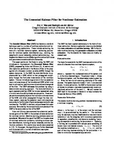
where 𝑀 denotes the number of Monte Carlo simulations and 𝑇 denotes the simulation time. We set 𝑇 as 100 seconds in 𝑚 is the first component of the true state in the simulation. x1,𝑘 𝑚 is its filtering estimate. 𝑚th simulation at time 𝑘 and x̂1,𝑘/𝑘 In fact, any element of x𝑘 can be chosen to illustrate the performance due to their symmetric status in x𝑘 and x𝑘 (1) is chosen in our simulation. We do 50 independent Monte Carlo runs under the same initial conditions. MSEs for state dimensions 𝑛 = 1 : 30 are shown in Figure 3, and single step running times of all filters for 30-dimensional system model are shown in Table 3. As shown in Figure 3, TUKF outperforms the 1st-SIF, 3rdSIF, 3rd-CKF, and 5th-CKF, especially for high state dimensions, and the proposed 3rd-QSIF and 5th-QSIF considerably outperform TUKF for moderate state dimensions in terms of filtering accuracy, and the proposed 3rd-QSIF, 5th-QSIF, and TUKF are almost consistent in filtering accuracy for high state dimensions. Besides, from Figure 3 and Table 3, we can see that the proposed 3rd-QSIF has higher filtering accuracy than the existing 1st-SIF with almost consistent computation demands. Simulation results illustrate that the proposed QSIF can effectively mitigate the nonlocal sampling problem.

6. Conclusion A QSIF method is proposed based on unbiased SSIR and FRIR in the paper. It can effectively solve the numerical instability problem, systematic error problem caused by nonlinear approximation, and nonlocal sampling problem for high-dimensional applications which exist in Gaussian filtering. Simulations of bearing-only tracking model and nonlinear filtering problem with different state dimensions show the advantages as compared with existing Gaussian filtering algorithms.

Conflict of Interests The authors declare that there is no conflict of interests regarding the publication of this paper.

Acknowledgments This work was supported by the National Natural Science Foundation of China under Grant nos. 61001154, 61201409, and 61371173, China Postdoctoral Science Foundation no. 2013M530147, Heilongjiang Postdoctoral Fund LBH-Z13052, and the Fundamental Research Funds for the Central Universities of Harbin Engineering University no. HEUCFX41307.

10

References [1] H. Jazwinski, Stochastic Processing and Filtering Theory, Academic Press, New York, NY, USA, 1970. [2] Y. C. Ho and R. C. K. Lee, “A Bayesian approach to problems in Stochastic estimation and control,” IEEE Transactions on Automatic Control, vol. 9, no. 4, pp. 211–221, 1975. [3] B. D. O. Anderson and S. B. Moore, Optimal Filtering, Prentice Hall, Englewood Cliffs, NJ, USA, 1979. [4] D. Simon, Optimal State Estimation: Kalman, H Infinity, and Nonlinear Approaches, John Wiley and Sons, New Jersey, NJ, USA, 2006. [5] H. W. Sorenson, “On the development of practical nonlinear filters,” Information Sciences, vol. 7, pp. 230–270, 1974. [6] I. Arasaratnam and S. Haykin, “Cubature Kalman filters,” IEEE Transactions on Automatic Control, vol. 54, no. 6, pp. 1254–1269, 2009. ˇ [7] M. Simandl, J. Kr´alovec, and T. S¨oderstr¨om, “Advanced pointmass method for nonlinear state estimation,” Automatica, vol. 42, no. 7, pp. 1133–1145, 2006. [8] D. L. Alspach and H. W. Sorenson, “Nonlinear Bayesian estimation using Gaussian sum approximations,” IEEE Transactions on Automatic Control, vol. AC-17, no. 4, pp. 439–448, 1972. [9] N. J. Gordon, D. J. Salmond, and A. F. M. Smith, “Novel approach to nonlinear/non-gaussian Bayesian state estimation,” IEE Proceedings F: Radar and Signal Processing, vol. 140, no. 2, pp. 107–113, 1993. [10] D. Guo and X. Wang, “Quasi-Monte Carlo filtering in nonlinear dynamic systems,” IEEE Transactions on Signal Processing, vol. 54, no. 6, pp. 2087–2098, 2006. [11] Y. Wu, D. Hu, M. Wu, and X. Hu, “A numerical-integration perspective on gaussian filters,” IEEE Transactions on Signal Processing, vol. 54, no. 8, pp. 2910–2921, 2006. [12] S. Julier, J. Uhlmann, and H. F. Durrant-Whyte, “A new method for the nonlinear transformation of means and covariances in filters and estimators,” IEEE Transactions on Automatic Control, vol. 45, no. 3, pp. 477–482, 2000. [13] S. J. Julier and J. K. Uhlmann, “Unscented filtering and nonlinear estimation,” Proceedings of the IEEE, vol. 92, no. 3, pp. 401– 422, 2004. [14] J. Dunik, O. Straka, and M. Simandl, “The development of a randomised unscented Kalman filter,” in Proceedings of the 18th IFAC World Congress, vol. 18, pp. 8–13, Milano, Italy, 2011. ˇ [15] O. Straka, J. Dun´ık, and M. Simandl, “Randomized unscented Kalman filter in target tracking,” in Proceedings of the 15th International Conference on Information Fusion (FUSION ’12), pp. 503–510, Singapore, September 2012. ˇ [16] J. Dun´ık, O. Straka, and M. Simandl, “Stochastic integration filter,” IEEE Transactions on Automatic Control, vol. 58, no. 6, pp. 1561–1566, 2013. [17] L. Chang, B. Hu, A. Li, and F. Qin, “Transformed unscented Kalman filter,” IEEE Transactions on Automatic Control, vol. 58, no. 1, pp. 252–257, 2013. [18] B. Jia, M. Xin, and Y. Cheng, “High-degree cubature Kalman filter,” Automatica, vol. 49, no. 2, pp. 510–518, 2013. [19] A. Genz and J. Monahan, “Stochastic integration rules for infinite regions,” SIAM Journal on Scientific Computing, vol. 19, no. 2, pp. 426–439, 1998. ˇ [20] M. Simandl and J. Dun´ık, “Derivative-free estimation methods: new results and performance analysis,” Automatica, vol. 45, no. 7, pp. 1749–1757, 2009.

Mathematical Problems in Engineering [21] P. J. Davis and P. Rabinowitz, Methods of Numerical Integration, Academic Press, New York, NY, USA, 1975. [22] A. H. Stroud, Approximate Calculation of Multiple Integrals, Prentice-Hall, Englewood Cliffs, NJ, USA, 1971. [23] G. W. Stewart, “The efficient generation of random orthogonal matrices with an application to condition estimators,” SIAM Journal on Numerical Analysis, vol. 17, no. 3, pp. 403–409, 1980. ˇ [24] J. Dun´ık, M. Simandl, and O. Straka, “Unscented Kalman filter: aspects and adaptive setting of scaling parameter,” IEEE Transactions on Automatic Control, vol. 57, no. 9, pp. 2411–2416, 2012. [25] Y. Zheng, O. Ozdemir, R. Niu, and P. K. Varshney, “New conditional posterior Cram´er-Rao lower bounds for nonlinear sequential Bayesian estimation,” IEEE Transactions on Signal Processing, vol. 60, no. 10, pp. 5549–5556, 2012.

Advances in

Operations Research Hindawi Publishing Corporation http://www.hindawi.com

Volume 2014

Advances in

Decision Sciences Hindawi Publishing Corporation http://www.hindawi.com

Volume 2014

Journal of

Applied Mathematics

Algebra

Hindawi Publishing Corporation http://www.hindawi.com

Hindawi Publishing Corporation http://www.hindawi.com

Volume 2014

Journal of

Probability and Statistics Volume 2014

The Scientific World Journal Hindawi Publishing Corporation http://www.hindawi.com

Hindawi Publishing Corporation http://www.hindawi.com

Volume 2014

International Journal of

Differential Equations Hindawi Publishing Corporation http://www.hindawi.com

Volume 2014

Volume 2014

Submit your manuscripts at http://www.hindawi.com International Journal of

Advances in

Combinatorics Hindawi Publishing Corporation http://www.hindawi.com

Mathematical Physics Hindawi Publishing Corporation http://www.hindawi.com

Volume 2014

Journal of

Complex Analysis Hindawi Publishing Corporation http://www.hindawi.com

Volume 2014

International Journal of Mathematics and Mathematical Sciences

Mathematical Problems in Engineering

Journal of

Mathematics Hindawi Publishing Corporation http://www.hindawi.com

Volume 2014

Hindawi Publishing Corporation http://www.hindawi.com

Volume 2014

Volume 2014

Hindawi Publishing Corporation http://www.hindawi.com

Volume 2014

Discrete Mathematics

Journal of

Volume 2014

Hindawi Publishing Corporation http://www.hindawi.com

Discrete Dynamics in Nature and Society

Journal of

Function Spaces Hindawi Publishing Corporation http://www.hindawi.com

Abstract and Applied Analysis

Volume 2014

Hindawi Publishing Corporation http://www.hindawi.com

Volume 2014

Hindawi Publishing Corporation http://www.hindawi.com

Volume 2014

International Journal of

Journal of

Stochastic Analysis

Optimization

Hindawi Publishing Corporation http://www.hindawi.com

Hindawi Publishing Corporation http://www.hindawi.com

Volume 2014

Volume 2014