QUASI-VERSUS PSEUDO-RANDOM GENERATORS

International Journal of Innovative Computing, Information and Control Volume 2, Number 3, June 2006

c ICIC International °2006 ISSN 1349-4198 pp. 1—31

QUASI-VERSUS PSEUDO-RANDOM GENERATORS: DISCREPANCY, COMPLEXITY AND INTEGRATION-ERROR BASED COMPARISON Syamal Kumar Sen, Tathagata Samanta and Andrea Reese Department of Mathematical Sciences Florida Institute of Technology Melbourne, FL, 32901, USA { sksen, tsamanta, areese }@fit.edu

Received May 2005; revised July 2005 Abstract. Presented here are several quasi- and pseudo-random number generators along with their numerical discrepancy, i.e., nonuniformity measure and computational/ time complexity. These generators have been compared and ranked based on discrepancy, complexity, and error in multiple Monte Carlo integrations. We believe that such a statistical comparison/ranking will be useful for solving real world problems where one needs to scan an s-dimensional region for an optimal solution of a mathematical program or multiple integrations. Keywords: Complexity, Error, Low discrepancy sequence, Monte Carlo integration, Pseudo-random number, Quasi-random number

1. Introduction. Non-existence of true random numbers in nature and artifact. The dictionary meaning of the word “random” is “made or done by chance without plan”. By this meaning it implies that no one will be able to predict the outcome out of several possible outcomes of any process. In nature, the outcome of any process cannot be strictly random since there is a relationship between the outcome and the inputs of the process through the process which obeys all the laws of nature perfectly and exactly. This observance of all the concerned laws of nature by any activity/process/method/algorithm is a hypothesis which has never been disproved. There is no question of breaking any law of the material universe under any circumstances at any time. Of course due to our limitations such as the lack of complete and/or perfect knowledge of the system and of all the laws governing the system, we, the human beings, are not able to explain or predict many phenomena/outcomes. If there is no process, then there is no outcome and hence no random numbers (RNs). Similarly, artificially too, we are not able to generate true RNs. Thus RN generation does exist neither in nature nor in digital computers (artifacts). Nature never produces any situation associated with a number that is random nor does it ever create chaos 1 . What we produce/generate in computers are thus called pseudo(implying false) RNs (PRNs) and/or quasi- (implying sub-) RNs (QRNs). Why quasi- over pseudo-random sequence. In many evolutionary approaches we need the explicit construction of point sets which fills out the s-dimensional (s-D) unit cube

1

The dictionary meaning of the word “chaos” is complete disorder or confusion. Chaos in science and engineering refers to an apparent lack of order in a system that nevertheless obeys certain laws and rules. This understanding of chaos is the same as that of dynamical instability. 1

2

S. K. SEN, T. SAMANTA AND A. REESE

as uniformly as possible. PRNs are often used for this purpose. However, PRNs tend to show some clustering effect (Galanti and Jung 1997). This effect will be more or less pronounced based on the PRN generator (PRNG) used. To obviate this undesired effect, consequently, QRNs were introduced. The generators of these numbers are designed and developed such that they produce more uniformly distributed random sequences. The general study of uniformly distributed sequences was initiated by Weyl (1916). In this context he introduced the notion of discrepancy (reflecting clustering) to measure the quality of uniformity of a finite random point set. Because of this property, QRNs are also referred to as low-discrepancy sequences or quasi-random (QR) sequences. QR sequence is more uniform than pseudo-random sequence. A random number generator (RNG) will be uniform in the interval [0, 1) if it produces outputs so that each trial has the same probability of generating a point (RN) on equal subintervals [0, 1/2) and [1/2, 1). In the case of PRNGs, it is possible for all of t trials (where t < 30, say t = 29 to denote small sample in the statistical sense2 ) to generate points so that they lie in the first half of the interval [0, 1/2), while the (t + 1)st point could lie in the other half [1/2, 1). This is not usually the case with the low discrepancy sequences or, equivalently, quasi-sequences, in which the outputs are constrained by a low-discrepancy requirement that has a net effect of points being generated in a highly correlated manner (i.e., the next point ”knows” where the previous points are). There are various explicit constructions, based on combinatorial methods, and algebraic number theory. The main challenge for the low discrepancy sequences is to avoid the multi-D clustering caused by the correlations between/among the dimensions. Having generated N (N ≥ 2) sample points, viz., QRNs, the next generated sample point will be distinct and away from any of the foregoing N sample points in a given region. This will tend to avoid clustering. Or, in other words, this will enhance the uniformity and reduce the discrepancy. Precisely, the sample points in a low discrepancy sequence are, “maximally avoiding” of each other. Zero-discrepancy sequence though most desirable is not essential. Ideally, a sequence having zero discrepancy is most desirable. However, there exist no QRN generators (QRNGs) that would produce QRNs resulting in zero discrepancy in mathematical sense in a digital computer. For real world applications we can generate enough QRNs to make discrepancy sufficiently low to obtain results that would be correct up to four significant digits (subject to the precision of the computer) since, in general, there exists no measuring device that has more than 0.005% accuracy3 . For any engineering application, low discrepancy sequences or, equivalently, QR sequences are sufficiently good. We do not have to go below certain discrepancy depending on the context. Accuracy and complexity based ranking for quasi-Monte Carlo methods. We compare the accuracy of the solution of the test4 problems, say numerical integration of single, double,

2

In the mathematical sense, however, the term small/large is relative. The term accuracy implies the relative error. If Q = quantity of higher order accuracy and Q0 = quantity of lower order accuracy then the accuracy (= relative error) in the quantity Q0 = |Q - Q0| / |Q|. Although the accuracy is the same as the relative error, these two terms are complementary, i.e., if the accuracy is more relative error is less and vice versa. 4 A test problem is one whose true (numerical) solution is already known. A real-world problem, on the other hand, is in general one whose true (numerical) solution is never known. For if it is known, then we do not have to do any computation. 3

QUASI-VERSUS PSEUDO-RANDOM GENERATORS

3

and triple variable functions by quasi-Monte Carlo (QMC) method or, equivalently, lowdiscrepancy MC method and pseudo-Monte Carlo (PMC) method. This comparison is done for a specified accuracy and hence for the consequent number of QRNs/PRNs. For k significant digit accuracy, if we need N QRNs for a single integration in [0, 1) then, for the same accuracy, we would require N 2 and N 3 QRNs for the corresponding (limits of integration for each variable are 0 and 1) double and triple integrations, respectively. A ranking of these methods is attempted based on accuracy/error and time complexity. The motive is to decide upon an appropriate quasi-randomized method to solve a realworld optimization/multiple integration problem so as to minimize relative error as well as time/computational complexity. We include an estimate of both error and complexity for any real problem that we solve. Error and Complexity: PRN versus QRN. The convergence rate of PMC Integration √ (PMCI) - how quickly the error decreases with the number of samples - is O(1/ N ). This implies that four times as many samples are required to cut down the error by 50%. Halton (Halton 1960; Morokoff and Caflisch 1994) showed the existence of infinite sequences in s-D cube which satisfy DN = O((log10 N )s /N ) where DN refers to the discrepancy of the first N terms of the random √ sequence. This is considered an important result since it offers hope that the PMC O(1/ N ) convergence can be improved significantly. We have taken the dimension s as 1 for the single integration and 2 for double integration. Determinism and error computation. QMC integrations (QMCIs) may be viewed as deterministic versions of PMCIs (Niederreiter 1992). The quasi-sequence injects determinism through deterministic points rather than random samples and through the availability of deterministic error bounds instead of probabilistic PMC error bounds. In QMCIs, deterministic nodes are selected in such a way that the error bound is as small as possible. The nature of QMC methods with these deterministic procedures implies that we get deterministic and thus guaranteed error bounds (Niederreiter 1992). It is thus always possible to determine beforehand an integration rule that yields a specified accuracy. For instance, for the single PMCI, we would need 100 times the RNs to reduce the error by a factor of 10 while for the single QMCI we would require hardly 10 times the RNs assuming constant discrepancy. It can also be seen that with the same computational effort, i.e., with the same number of function evaluations (which could be computationally intensive in numerical integration), the QR sequence achieves a significantly higher accuracy than the pseudo-random (PR) sequence. The detailed relative computational complexity (amount of computations) will be provided along with the examples. QR sequences: existing literature. Several methods for producing QR sequences have been developed (Halton 1960; Sobol 1967; Faure 1982; Niederreiter 1988). Fox (1986) compared the efficiency of Halton and Faure QRNGs and a linear congruential PRNG, Bratley, Fox, and Niederreiter (1992) included in this comparison the Sobol QRNG. QR/low-discrepancy sequences along with their measures and applications were considerably discussed (Hua and Wang 1981; Sarkar and Prasad 1987; Niederreiter 1988, 1992; Shirley 1991; Struckmeier 1995; Galanti and Jung 1997, Kocis and Whiten 1997; Henderson et al. 2000). There are many computational problems such as those in linear and

4


nonlinear optimization (Hickernell and Yuan 1997), numerical multiple integration (Sloan and Joe 1990), computer graphics (Shirley 1991), image processing (Hannaford 1993), computational finance (Papageorgiou and Traub 1997), and linear algebra (Mascagni and Karaivanova 2000) where these sequences are more desirable for better quality of numerical results through algorithms that use these sequences. We present the foregoing QRNGs in Section 2 while single, double and triple Monte Carlo integrations (MCIs) using these QRNGs and also the PRNGs Rand (Matlab), Simscript (Sims), R250, and Whlcg are described in Section 3. The role of discrepancy in pseudo- and quasi-random sequences along with its theoretical and computational definitions is discussed in Section 4. Also investigated in this section are the minimal discrepancies and also the number of RNs needed to be generated in pseudo- and quasi-random sequences. Numerical experiments with statistical tables and graphs to highlight the scope of QRNs over PRNs constitute Section 5, ranking of both PRNGs and QRNGs comprises Section 6 while conclusions are included in Section 7. All the relevant Matlab programs are appended for ready check/use. 2. Random Number Generators. 2.1. Quasi-random numbers. We describe the Halton, the Sobol, the Faure, and the Niederreiter (Nied) QRNGs. All these QRNGs have generated QRNs in the semi-closed interval [0, 1). A generalization to any other interval [a, b) is immediate since the new QRN will be a + r(b − a), where r is the QRN in [0, 1). Halton QRNG. The Halton sequence (Halton 1960; Halton and Smith 1964) is a class of multi-D infinite sequence which is generated using a prime base depending on each dimension s. For s = 1, base 2 (the Van der Corput base 2 sequence (Van der Corput 1935) is also the first dimension of the Halton sequence) is used, for s = 2, base 3 is used while s = 3, base 5 is used. Thus, for s = n, the nth prime number will be the base. For example, s = 28, the base will be 107, i.e., the 28th prime number starting from the prime number 2. Any integer n can be written uniquely in base p, i.e., n=

m X

a j pj

(1)

j=0

where m is the lowest integer that makes aj = 0 for all j > m and 0 ≤ aj < p. Although the base p can be any positive integer for uniqueness for the foregoing representation (1), in Halton sequence p is chosen as a prime. This is because the finite field arithmetic (multiplication/division) will have unique representation only in prime base. To generate a Halton sequence, a decimal integer n (n = 0, 1, 2, . . . ) is represented in base p where p is a prime number. To obtain a value in [0, 1), the digits are reversed and a decimal point is added by using φ(n) =

m X

aj p−j−1

(2)

j=0

Example: Consider the decimal integer n = 13, dimension = 1 and so the prime base = 2. Then n = 13 = 1 × 23 + 1 × 22 + 0 × 21 + 1 × 20 , so the number in base 2


5

is 1101. Reflecting about the radix point, obtain 0.1011 and the consequent decimal fraction φ(11) = (0.1011)2 = 1 × 2−1 + 0 × 2−2 + 1 × 2−3 + 1 × 2−4 = (11/16)10 = 0.6875 (up to 4 decimal places). Similarly, for the decimal integer n = 11, dimension = 2 and so the prime base = 3. Then n = 11 = 1 × 32 + 0 × 31 + 2 × 30 , so the number in base 3 is 102. Reflecting about the radix point, obtain 0.201 and the consequent decimal fraction φ(10) = (0.201)3 = 2 × 3−1 + 0 × 3−2 + 1 × 3−3 = (19/27)10 = 0.7037 (up to 4 decimal places). It can be seen that the Halton sequence for one dimension (always base 2) is identical to the Van der Corput (always base 2) sequence. The base of each Halton sequence increases as we increase the dimension. Larger dimension implies larger base which results in longer cycle and more computational time. The length of the cycle equals the base of the dimension, i.e., for base 2 (representing dimension = 1) the length of the cycle is 2. Similarly, for base 173 (representing dimension = 40) the length of the cycle is 173. The cycle numbers for base 2 along with generated QRNs and cycle length are depicted in Table 1 while those for base 3 are represented in Table 2. Table 1. Dimension s= 1, i.e., base = 2 Cycle Generated Cycle Number QRNs Length 1 0 1/2 2 2 1/4 3/4 2 3 1/8 5/8 2 4 3/8 7/8 2 5 1/16 9/16 2 6 5/16 13/16 2 7 3/16 11/16 2 8 7/16 15/16 2

Table 2. Dimension s = 2, i.e., base = 3 Cycle Number 1 2 3 4 5 6 7 8 9

Generated Cycle QRNs Length 0 1/3 2/3 3 1/9 4/9 7/9 3 2/9 5/9 8/9 3 1/27 10/27 19/27 3 4/27 13/27 22/27 3 7/27 16/27 25/27 3 2/27 11/27 20/27 3 5/27 14/27 23/27 3 8/27 17/27 26/27 3

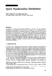
For high dimensions the sequence is overly sensitive to the starting values of n, because reflection about the decimal point generates values that are more densely populated near zero, i.e., they cluster near zero. So as the dimension of the sequence increases the number of discarded points also increases. Further as the dimension s increases the space to be filled in becomes large needing many more points to be generated - these will reduce clustering effect (Figures 1-4). We have used Matlab program scatterplot.m with maxcount 1000 (1000 pairs of QRNs) that uses halton1 and halton2 with dimensions 1 and 2 respectively in Figure 1, those with dimensions 7 and 8 in Figure 2, and those with dimensions 27 and 28 in Figure 3. Figure 4, however, differs from Figure 3 only in maxcount which is taken as 10000 (10000 pairs of QRNs). Sobol QRNG. The Sobol sequence (Sobol 1967) uses base 2 for all dimensions. In higher dimensions it is a reordering of the first dimension. Because of this the higher-D Sobol sequence eliminates the problem of clustering caused by the Halton and the Faure sequences. Any integer n can be written uniquely in any base. In base 2, it is

6


Figure 1. Halton points (ordered pair of QRNs) in dimension 1 - dimension 2 coordinates




n=

M X

ai 2i

i=0

where M is the smallest number greater than or equal to log2 n and ai is 0 or 1. The Sobol sequence uses linear recursions (3) and (5) below (Bratley and Fox 1988). A primitive polynomial of degree d is P = xd + h1 xd−1 + h2 xd−2 + ... + hd−1 x + 1 where hj , (j = 1, 2, . . . , d-1) is 0 or 1. For example, the primitive polynomial P = x3 + x2 + x + 1 has h1 = 1 and h2 = 1.


7

We generate all mi , i = 0, 1,. . . , M using the coefficients hj (j = 1, 2, . . . , d-1) of the primitive polynomials of modulo 2 and a recursion for i > d mi = 2h1 mi−1 ⊕ 22 h2 mi−2 ⊕ ... ⊕ 2d−1 hd−1 mi−d+1 ⊕ 2d mi−d ⊕ mi−d (3) where ⊕ is the bitwise exclusive-or (XOR) operator defined by1 ⊕ 0 = 0 ⊕ 1 = 1 and 1 ⊕ 1 = 0 ⊕ 0 = 0. Observe that the value of mi is an odd integer that lies in [1, 2i −1]. The direction numbers v(i), where i = 1, 2, . . . M, in the finite field with elements {0, 1} is given, in base 2, by Then the nth

(4) v(i) = mi /2i element of the Sobol sequence (QRNs), φ(n), can be generated by using

φ(n) = a1 v(2) ⊕ a2 v(3) ⊕ ... ⊕ ai v(i) (5) For faster generation of Sobol QRNs, Antonov and Saleev (1979) implemented (5) in a different way, known as Gray code. The algorithm for generating Gray code is by the bitwise exclusive-or operation of n and n/2, i.e.,φ(n) = n ⊕ (n/2). Consequently, the modified version of (5) is φ(n + 1) = φ(n) ⊕ v(i) (6) where v(i) is the ith direction number and i is the rightmost zero bit in the base 2 expansion of n. Example: To generate the Sobol QRNs, choose a primitive polynomial, say, P = x3 + x2 + 1 = 1x3 + 1x2 + 0x + 1, where the coefficients h1 = 1and h2 = 0. Using (3) we have, mi = 2mi−1 ⊕ 23 mi−3 ⊕ mi−3 . Choose the first three mi ’s arbitrarily as m1 = 1, m2 = 3, and m3 = 7. Then m4 = 2m3 ⊕8m1 ⊕m1 = 14⊕8⊕1 = 1110⊕1000⊕0001 = 0111 = 7. Similarly m5 = 2m4 ⊕ 8m2 ⊕ m2 = 14 ⊕ 24 ⊕ 3 = 01110 ⊕ 11000 ⊕ 00011 = 10101 = 21, m6 = 2m5 ⊕ 8m3 ⊕ m3 = 42 ⊕ 56 ⊕ 7 = 101010 ⊕ 111000 ⊕ 000111 = 010101 = 21, and so on. Using (4), find v(1) = 1/21 = 1/2 = 0.1, v(2) = 3/22 = 3/4 = 0.11, v(3) = 7/23 = 7/8 = 0.111, and so on. Now the Sobol QRNs are generated with the gray code suggested by Antonov and Saleev (1979) as follows. Choose φ(0) = 0, for n = 0 the right most zero bit in base 2 expansion of n is i = 1, then the first QRN is φ(1) = φ(0 + 1) = φ(0) ⊕ v(1) = 0.0 ⊕ 0.1 = 0.1 = 1/2. For n = 1 the right most zero bit in base 2 expansion of n is i = 2, then the second QRN is φ(2) = φ(1 + 1) = φ(1) ⊕ v(2) = 0.10 ⊕ 0.11 = 0.01 = 1/4. For n = 2 the right most zero bit in base 2 expansion of n is i = 1, then the third QRN is φ(3) = φ(2 + 1) = φ(2) ⊕ v(1) = 0.01 ⊕ 0.10 = 0.11 = 3/4 and so on. Faure QRNG. The Faure sequence (Faure 1982) is also an s-D sequence but, unlike the Halton sequence, all its dimensions use the smallest prime ≥ s as the base. The one-D sequence uses base 2. It can be seen that each of the Van der Corput base 2 sequence and the Halton base 2 sequence is the same as the Faure base 2 sequence for the first dimension. The two-D Faure sequence also uses base 2 (the smallest prime number ≥ 2). In this case, both second dimension and first dimension sequences use base 2 but the second dimension sequence is a reordering of the values in the first dimension. The three-D Faure sequences use base 3. In this case, the second and the first dimensions

8


also use base 3 but they will have different reordering. Likewise the fourth-D and fifth-D sequences use base 5 but will have different reordering of the first sequence generated. The sequence is constructed as follows. Each integer n (n = 0, 1, 2, . . . ) is represented in base p, except p is now chosen as the smallest prime number ≥ the dimension s and ≥ 2. To obtain a value in [0, 1), the digits are reversed and then a decimal point is inserted in front of the left-most digit (similar to the Halton sequence). Any integer n can be written uniquely in base p, as in (1). Let the combinations Cij = j!/i!(j − i)!. Digits aj thus obtained are reordered (see the example below) to obtain the new sequence bi using " m # X j bi = Ci (s − 1)j−i aj mod p i = 0, 1, 2, . . . , j (7) j≥i

To obtain a value φ(n) in [0, 1), these new coefficients bi are reversed and a decimal point is added before the left-most digit as in (2). Example: Let n = 10, dimension s = 2, so base p = 2. Then n = 10 = 1 × 23 + 0 × 22 + 1×21 +0×20 , so the number is (a3 a2 a1 a0 )2 = (1010)2 . Note that (s−1)j−i = (2−1)j−i =1. ⎡ ⎡ 0 ⎤ ⎤ ⎡ ⎤ a0 b0 C0 C01 C02 C03 ⎢ ⎢ b1 ⎥ ⎢ ⎥ C11 C12 C13 ⎥ ⎥ = (s − 1)j−i × ⎢ 0 ⎥ ⎢ a1 ⎥ mod p b4 (n) = ⎢ 2 3 ⎦×⎣ ⎣ b2 ⎦ ⎣ 0 0 C2 C2 a2 ⎦ 3 b3 0 0 0 C3 a3 ⎡ ⎤ ⎡ ⎤ ⎡ ⎤ 1 1 1 1 0 0 ⎢ 0 ⎥ ⎢ 0 1 2 3 ⎥ ⎢ 1 ⎥ ⎥ ⎢ ⎥ ⎢ ⎥ =1×⎢ ⎣ 0 0 1 3 ⎦ × ⎣ 0 ⎦ mod 2 = ⎣ 1 ⎦ 0 0 0 1 1 1

so the binary number 1010 after reordering and with a binary point at the extreme left becomes 0.0011. Hence the corresponding decimal number is φ(10) = 0.0011 = 0 × 2−1 + 0 × 2−2 + 1 × 2−3 + 1 × 2−4 = 3/16 = 0.1875 which is the required QRN in [0, 1). The base p of each Faure sequence increases with the increase in dimension s, but the problem starts when the dimension is large. As s increases the space to be filled in becomes large. Larger dimension implies larger base which results in longer cycle and more computational time. However, in a higher dimension, for the same number of QRNs generated, Faure fills gap more uniformly than Halton. This is because Halton in dimension 28 uses base as 107 (which is also the cycle length) while Faure in dimension 28 uses base as 29. For large dimensions the sequence is overly sensitive to the starting values of n, because reflection about the decimal point generates values that cluster near zero (Bratley et.al. 1992). To minimize this effect Faure (Bratley and Fox 1988) suggested discarding the first n = p4 − 1 points, where p is the base of the sequence. So as the dimension of the sequence increases the number of discarded points also increases. If p = 29 then the first 294 − 1 = 707280 QRNs will be discarded. Niederreiter QRNG. A QR sequence in base b generated by Niederreiter’s method (1988) has the property that strings of bm (m is any integer ≥ 0) successive points divide themselves evenly among certain elementary intervals in base b. To obtain a (t, s) sequence in


9

base b, let B = {0, 1, ..., b − 1} for the set of digits in base b, where b ≥ 2, s ≥ 1, and both are integers. Then choose the following. i) a commutative ring R with identity and card(R) = b, ii) bijections ψr : B → R for r = 0, 1, . . . , with Ψr (0) = 0 for all sufficiently large r, iii) bijections λij : R → B for i = 1, 2, . . . , s and j = 1, 2, . . . , with λij (0) = 0 for 1 ≤ i ≤ s and sufficiently large j, (i) (i) iv) elements cjr ∈ R for 1 ≤ i ≤ s, j ≥ 1, r ≥ 0, where for fixed i and r we have cjr = 0 for all sufficiently large j. To generate xn (Bratley et al. 1992, 1994) let the base b representation of n − 1 be n − 1 = aR−1 aR−2 ...a1 a0 , ak ∈ B where n = 1, 2, . . . . Then xn is, as a base b fraction, xn = 0.d1 d2 ...dR , where dj =

R−1 XY r=0

(cjr , ar ),

dk ∈ B

1 ≤ j ≤ R.

In practice we compute an integer Qn whose base b representation is Qn = d1 d2 ...dR and set xn = Qn /bR . However, the following simpler form (Judd 1999) of Nied QRNG is more attractive for computer implementation. Let θ be the fractional part of the real number θ. The Nied QR sequence in Rs is then xn = {n.2s/(s+1) }, where, for each dimension s, the subscript n will take values 1, 2, 3, . . ., N , (N being the number of RNs to be generated). Example For s = 1 and N = 3 we have x1 = {1.21/2 } = {1.4142} = .4142, x2 = {2.21/2 } = .8284, x3 = {3.21/2 } = .2426. For s = 2 and N = 3 we have x1 = {1.22/3 } = {1.5874} = .5874, x2 = {2.22/3 } = .1748, x3 = {3.22/3 } = .7622 and so on. 2.2. Pseudo-random numbers. Most of the commonly used PRNGs are based on linear congruential (LCG) methods while others on generalized feedback shift register procedure, subtract with borrow technique, and combined linear congruential methods (Knuth 1981; L’Ecuyer 2001; Lakshmikantham et. al. 2005). These generators are distinct and are used in the programming languages Apple, Bcpl, Derive, Glim, Matlab 5, Minstd, Simscript, Turbo C++, Turbopascal, Urn12, and Matlab 6.5. Without any ambiguity we call these generators by their respective programming language names (Lakshmikantham et. al. 2005). The other generators are R250, Whlcg, Ranecu, Lelcg, Randu, and Drand48 (Lakshmikantham et. al. 2005). We have considered the generators Simscript (linear congruential generators), R250 (generalized feedback shift register generator), Matlab Rand (subtract with borrow generator), and Whlcg (combined linear congruential generator) for the purpose of comparison with QRNGs. It can be seen that each of the foregoing

10


four generators is based on a distinct well-known method. For the sake of a comparison, we think that we will get a clear picture of where the QRNGs stand with respect to the PRNGs in solving problems that need the scanning of an s-D region. Figures 5 and 6 show the plot of PR points on a square. Observe that the PR points in Figures 5 and 6 are less uniformly distributed (through visual perception) than the QR points in Figure 1 implying greater degree of clustering effect in PRGs. In Figures 5 and 6, we have used Matlab program scatterplot.m in which maxcount =1000 (1000 pairs of PRNs).

Figure 5. R250 pseudorandom points in 2-D coordinates (1000 pairs of PRNs)

Figure 6. Rand pseudorandom points in 2-D coordinates (1000 pairs of PRNs)

3. Quasi- and Pseudo-Monte Carlo Integrations. We consider here single, double, and triple integrations, viz.,

I1 =

Z1

f (x) dx,

I2 =

0

Z1 Z1 0

f (x, y) dx dy,

I3 =

0

Z1 Z1 Z1 0

0

f (x, y, z) dx dy dz.

(8)

0

The generalization to any multiple integrations beyond three dimensions is straightforward. It may be seen that the interval [a, b], [0, ∞), or (-∞, ∞) can always be mapped onto finite intervals such as the interval [0, 1], [0, 1), or (0, 1) respectively by the change of interval of integration5 (Krishnamurthy and Sen 2001). 5

It may be seen that while 0 is a number (representing graphically a point), ∞ is not a number conventionally. The semi-open interval [a, ∞) can only be mapped onto the semi-open interval [0, 1). Mathematically speaking exactly the point ‘1’ is not included in this interval, while in the engineering sense it may be included and we may write this interval as the closed interval [0, 1]. Consider for example R∞ R1 the integral I = 1/x3 dx = (t − 1) dt = 1/2. In this integral, [1, ∞) may be assumed to have been 1

0

mapped onto the closed interval [0, 1] in the engineering sense, this is incorrect in the strict mathematical sense though. Observe that a point is something that has no length, no width, and no height but it exists. Although this definition has inherent contradiction, it is not difficult to grasp the concept of point. A point adjacent to the point ‘1’ is certainly not the point ‘1’ yet the distance between these two points R∞ Rk may be assumed zero. Also observe that I = 1/x3 dx = lim 1/x3 dx in strict mathematical sense. 1

k→∞ 1


11

Summation based MC integration. QMCI (Morokoff and Caflisch 1995) is the same as the PMCI except that PRNs are replaced by QRNs. For the description of the probability based PMCI, refer Lakshmikantham et al. (2005). In this description, we have used probability of a dart (representing a random point) hitting the area under the curve represented by the function f (x)(orf (x, y)orf (x, y, z)). The integral evaluation will be better if the points are uniformly scattered in the entire rectangular area (or cuboid or rectangular hyperspace of dimension four 6 ), that is, if the points are spread uniformly all over the area. One disadvantage of this procedure is that we need to consciously take care of the function on the positive as well as the negative quadrants separately. To obviate this disadvantage, we write any integral (single or multiple) with any limits of integration [a, b] to one with limits of integration [0, 1]. We then use a summation (single or multiple) formula below to obtain the integration value. This summation procedure is a much simpler form of MCI in which we do not have to consciously worry about the negative/positive value of the function F (t). Summation formula for MC integration: single, double, and triple. The MCI is to use random points for the numerical evaluation of an integral. Consider the computation of I1 in (8). The standard MC estimate of the integral is equal to the average value of the function taken over N points selected randomly from the unit interval [0, 1]. The strong law of large numbers states that a series of independent and identically distributed (iid ) random variables, normalized by the number of terms in the series, will converge to the mean of any one of the terms in the series consisting of partial sums sN . So this estimate tends to the true value of the integral √ as N tends to infinity. From the Central Limit theorem, the standard error tends to1/ N . The only restriction on the function f (x) is that it be square integrable7 . The unbiased Monte Carlo estimate is N 1 X f (xi ) I1 = N i=1

(9)

Limit theorem the where xi are chosen uniformly randomly in [0, 1]. By the Central P variance Var of the estimateI1 is defined as V ar = (1/(N − 1)) (f (xi ) − I 1 )2 , where the summation is over i = 1 to N , which is a measure of the extent to which f (x) deviates from its average value over the √ range of integration. A measure of the error in the integration value I1 given as E = ( V ar)/N . The error is due to the fact that it is an average of randomly generated points and so itself random. In real world situation we do not have the knowledge of the exact/true numerical result of the integral. To get an estimate of the error/spread, we compute variance and hence the error E as given above. 6

Cuboid is rectangular parallelepiped while the rectangular hyperspace of dimension four will be a hypercube when all four dimensions are equal. We cannot comprehend geometrically objects of dimension four and above although the mathematical extension to dimension four and much greater than four is extremely useful in solving real-world linear and nonlinear problems. R∞ 2 7 A function f (x) is square integrable if |f (x)| dx is finite. −∞

12


However, another way (Lakshmikantham and Sen 2005) of estimating the relative error (RE ) in I1 is to compute I1 with N (N = 2000, say) QRNs. Call this I1 as ILA , which is a quantity of lower order accuracy. Likewise, compute I1 with M (M = 20000, say) QRNs. Call this I1 as IHA , which is a quantity of sufficiently higher order accuracy. Then the RE in ILA = (|IHA − ILA | / |IHA |) × 100. This estimate of the error is universally varied for any real-world numerical integration (MC as well as non-MC). Let us assume that the period of the sequence of PRNs generated is sufficiently large √ (long). Then the error for summation based PMCI is O(1/ N ) (Bratley et al. 1992), where N is the total number of PRNs generated, independent of the dimension of the integral. The 2-D integral I2 in (8) is approximated by the double summation I2 =

q q q q 1 XX 1 XX f (x , y ) = f (xi , yj ) i j q 2 i=1 j=1 N i=1 j=1

(10)

where N = q 2 is the number of RNs generated, while the 3-D integral I3 in (8) is approximated by the triple summation q q q q q q 1 XXX 1 XXX I3 = 3 f (xi , yj , zk ) = f (xi , yj , zk ) q i=1 j=1 k=1 N i=1 j=1 k=1

(11)

where N = q 3 is the number of RNs generated. The QRNs improve the accuracy of the integration as well as complexity so long as the dimension of integration is not very high, say 40 (Galanti and Jung 1997). Disadvantages of QRNs. QMC methods are valid for integration problems, but may not be directly applicable to simulations, due to the correlations between the points in neighboring dimensions of a QR sequence. The improved accuracy of QMCIs is generally lost for problems of high dimension (due to clustering), say 40, or problems in which the integrand is violently fluctuating in the interval of integration. 4. Discrepancy. It is a measure of the lack of uniformity or lack of equidistribution of points placed in a set, usually in the unit hypercube [0,1)s . The most widely studied discrepancy measures are based on the Lp norms (p = 2, or p = ∞). With p = 2 this discrepancy is called the L2 -discrepancy. When p = ∞, this discrepancy is called the ∗ . The discrepancy of the point set {xi }i = 1,...,N ∈ [0, 1)s is star-discrepancy DN ¯ ¯ ¯ sup ¯¯ A(E, N ) s DN = − λ(E)¯¯ ¯ E N where E = [0, t1 ) × ... × [0, ts ), 0 ≤ tj ≤ 1, j = 1, ..., s is an s-D hyper-rectangle8 , the parameter λ(E) is the Lebesgue measure of E, which is the s-D space under the curve y = f (x1 , x2 , . . . , x s ) (Niederreiter 1992). The parameter A(E, N ) is the number of xi contained in E and hence A(E, N )/N is the fraction of xi contained in E, and the discrepancy is the largest9 difference between A(E, N )/N andλ(E). 8

The hyper-rectangle will be the hypercube if all tj are equal to one. The term sup denotes supremum which implies maximum or largest when n is finite. For different independent runs (i.e., the same MCI computed several times), the value of A(E, n)/n will be different. We consider the one which is the largest in magnitude. 9


13

For any N > 1 and sequence {x i }, let {xi }i = 1,...,N denote the first N points of the ∗ ≤ C s (log 10 N )s /N , where the constant Cs depends only on sequence {x i }. If we have DN the dimension s, then the sequence {x i }, is called a low-discrepancy sequence. Niederreiter (1992), Press et al. (1992), and Drmota and Tichy (1997) may be referred. The construction of QR sequences is based on minimizing their discrepancy. While seemingly complicated, for a 1-D point set the star-discrepancy is the Kolmogorov-Smirnov statistic based on the uniform distribution. The test procedure follows the steps below (Banks 1996). Step 1 : Rank the data from smallest to largest, so that R1 ≤ R2 ≤ ... ≤ RN

Step 2 : Compute +

D = max

1≤i≤N

Step 3 : Compute

½

¾ i − Ri , N

½ ¾ i−1 D = max Ri − 1≤i≤N N −

D = max(D + , D − ) (12) The Koksma-Hlawka inequality (Niederreiter 1992) is essentially the only theoretical tool for estimating the accuracy (implying non-discrepancy) of a QMC estimate, and was motivated by numerical integration, but this is very difficult to implement. The discrepancies for the PRNs and QRNs are, respectively, ³p ´ ∗ (P RN ) ∈ O (log10 log10 N )/N (13) DN ∗ (QRN ) ∈ O ((log10 N )s /N ) (14) DN For further information on computing the discrepancy, refer Dobkin and Eppstein (1993).

5. Numerical Experiments. We have computed the discrepancy of each RNG in one dimension based on the Kolmogorov-Smirnov test. We have compared the RNGs using the MCI of (i) a single variable function as well as (ii) a double variable function. Such a comparison is possible since embedded in the integration is an RNG. Consider (i) the single variable function f (x) = x2 , with the limits of integration [0, 1] and (ii) the double variable function f(x, y) = x 2 + y 2 , with the limits of integration [0, 1] for each of the variables x and y. The true integration value for x2 is 0.333333333333333 while that for x2 + y 2 is 0.666666666666667. We have then obtained the computed accuracy and the time complexity for each RNG. Based on these results we tried to rank them. Comparing Discrepancy. We compute the discrepancies from (12) for different QRNGs and PRNGs as in Table 3. From Table 3, the ranking of the RNGs based on the average discrepancies over a large range (20 to 200000) of RNs generated is: Nied (rank 1, i.e., the best implying least discrepancy), Sobol, Halton, Faure, Sims, R250, Derive, Whlcg, and Rand (rank 8 implying largest discrepancy). However, for a smaller range (say, 20 to 2000) of RNs this ranking will change. A visualization of these discrepancies is given in Figure 7.

14


Table 3. QRNGs and PRNGs: discrepancy measure for various RNs generated Points (# of RNs) Halton (base = 3) Faure (base = 2) Sobol Nied Sims R250 Rand Whlcg

20 .09774 .10625 .07500 .06472 .12487 .19119 .25570 .25028

200 .00868 .02031 .01031 .00841 .06429 .03834 .05531 .05015

2000 .00156 .00171 .00168 .00127 .02570 .02677 .01435 .01449

20000 .00015 .00017 .00015 .00013 .00918 .00419 .00589 .00818

200000 Average discrepancy .00003 .02163 .00002 .02569 .00001 .01743 .00002 .01491 .01653 .04811 .00219 .05254 .00339 .06693 .00362 .06534

Figure 7. Number of RNs versus discrepancy for QRNGs and PRNGs

Comparing computed accuracy with expected accuracy/error in integration with Halton and Rand. We have included the probability based single MCI error in Tables 4 and 6, and the summation based single MCI error in Tables 5 and 7. We have used the Halton QRNG in Tables 4 and 5 and Rand PRNG in Tables 6 and 7. Specifically, in Tables 4-7 we have dimension s = 1, Error E in I1 is O(((log10 N )1 /N ) × 100) for large N , where N = no. of RNs, CA = computed accuracy = (|true I1 − computed I1 |/|true I1 |) × 100 = computed relative error (in percent), SE = standard error expected based on RNs √ generated = O((1/ N ) × 100), CI1 = Computed I1 . In Tables 4-9 we have considered the 1-D integration I1 of the function f (x) = x2 over the interval [0, 1]. It may be seen, from Tables 4 and 5, that the computed relative error CA tallies well with the order of QMCI error E which is significantly better (reduced) than the standard error SE, where both SE and E are only based on the number of RNs generated. Also observe that from Tables 6 and 7, the computed relative error CA does not tally very


Table 4. Probability based QMCI error N

CI1

CA

2×10 2×102 2×103 2×104 2×105

.30000 .32500 .33450 .33325 .33332

10.00 2.500 0.350 0.025 0.003

Order Order of E of SE 6.505 22.361 1.151 7.071 0.165 2.236 0.022 0.707 0.003 0.224

15

Table 5. Summation based QMCI error N

CI1

CA

2×10 2×102 2×103 2×104 2×105

.32719 .33069 .33313 .33330 .33333

1.844 0.792 0.062 0.010 0.000

Order Order of E of SE 6.505 22.361 1.151 7.071 0.165 2.236 0.022 0.707 0.003 0.224

well with order of SE ; this implies reduced uniformity (more discrepancy). However, the numerical differences between CA and SE are still tolerable. Table 6. Probability based PMCI error N 2×10 2×102 2×103 2×104 2×105

CI1 .35000 .33000 .34250 .33190 .33385

CA Order of E 5.000 22.361 1.000 7.071 2.750 2.236 0.430 0.707 0.154 0.224

Table 7. Summation based PMCI error N 2×10 2×102 2×103 2×104 2×105

CI1 CA Order of E .47744 43.231 22.361 .35884 7.651 7.071 .33295 0.114 2.236 .33448 0.344 0.707 .33397 0.191 0.224

Number of RNs versus accuracy/error and time complexity in single integration. Assuming sufficiently long period of the random sequence we find that there exists a relationship between the RNs used and the corresponding accuracy in summation based MCI. This relationship for the single MC method is approximately linear for QRNs as depicted in Table 8. However this relationship is rather fluctuating for PRNs as shown in Table 9. Such a difference is attributed, in the behavior of PRNs and QRNs, to the difference in discrepancies of these RNs. The time complexities (TCs) have been shown in seconds only up to two decimal places. Hence 0.00 second in Table 9 necessarily implies a positive time in milliseconds. So far as the time complexities among the QMCIs are concerned we see from Table 8 that Nied is distinctly the best (least time of computation) much better than Halton/Faure and Sobol QRNGs while Halton/Faure QRNG is clearly better than Sobol in single integration. Time Complexities for 1-D QMCI and 1-D PMCI using QRNGs and PRNGs for 200000 RNs are depicted using a bar chart in Figure 8, in which Rand (Matlab) PRNG is the best while Nied QRNG is the next best. We have not considered PMCI using R250 PRNG in the bar chart (Figure 8) because of excessive time complexity due to exclusiveor operations embedded in it. In other words, R250 PRNG is not recommended to be used when number of RNs used for 1-D PMCI is large. However, for 2-D PMCI the TC of R250 is comparable to those of the other PRNGs and may be used. In Tables 8 and 9, we have true I1 = .333333 and EA = expected accuracy = 1/(# of RNs), CA = computed accuracy = (|true I1 − computed I1 |/|true I1 |) × 100 (%), TC = Time Complexity, observe that Halton (dim = 1) = Faure (dim = 1) = Van der

16


Corput. The time complexity has been computed using Matlab 7 on an Intel Pentium 4 Processor 3.1 GHz, 592MHz, 1 GB RAM and 1MB L2 Cache Table 8. QRNs versus expected accuracy of MC single integration I1 of x2 over [0, 1] # of QRNs 20 200 2000 20000 200000 EA (%) 5 .5 .05 .005 .0005 Halton I (dim=1) .32719 .32984 .33304 .33326 .33332 CA (%) 1.84448 1.04763 .08828 .02211 .00294 TC (sec) 0.02 0.03 0.05 0.38 4.31 Sobol I (dim=1) .32832 .33001 .33340 .33333 .33333 CA (%) 1.50391 .99689 .01985 .00055 .00018 TC (sec) 0.03 0.09 0.21 1.94 19.51 Nied I (dim=1) .32854 .33154 .33296 .33331 .33333 CA (%) 1.43918 .53773 .11182 .00711 .00046 TC (sec) 0.01 0.02 0.04 0.08 0.50 Table 9. PRNs versus expected accuracy of MC single integration I1 of x2 over [0, 1] # of PRNs EA (%) Sims I CA (%) TC (sec) R250I CA (%) TC (sec) Rand I CA (%) TC (sec) Whlcg I CA (%) TC (sec)

20 200 2000 20000 200000 5 .5 .05 .005 .0005 .32843 .35182 .34248 .33088 .32779 1.47135 5.54494 2.74273 .73700 1.66176 .00 .02 .02 .14 1.27 .27519 .33574 .32462 .33311 .33289 17.4421 .72143 2.61331 .06843 .13402 .00 .02 .03 2.48 405.34 .31055 .34326 .32916 .33142 .33295 6.83450 2.97689 1.25260 .57357 .11433 .00 .00 .01 .02 .02 .27331 .34030 .33598 .33535 .33502 18.0077 2.09041 .79271 .60464 .50523 .00 .02 .05 .38 3.75

In Tables 10 and 11, we have true I2 = .666667 and, where EA = expected accuracy = 1/(# of RNs), CA = computed accuracy = (|true I2 − computed I2 |/|true I2 |) × 100 (%), TC = Time Complexity. The time complexity has been computed using Matlab 7 on an Intel Pentium 4 Processor 3.1 GHz, 592MHz, 1 GB RAM and 1MB L2 Cache. For sufficiently large number of QRNs the time complexity (TC) for QMCI will be proportionately increased. For example, if number of QRNs is 2000002 and is increased by a factor of 100 to 20000002 then the TC will also increase by roughly 100 times. However for small number of QRNs such an increase will be significantly less (than the factor 100) because of the implicit (approximately) constant overhead in computation.


17

Figure 8. Time Complexity for 1-D QMCI and 1-D PMCI using QRNGs and PRNGs for 200000 RNs where Hal = Halton(QRNG), Fau = Faure(QRNG), Rand(PRNG), Sims = Sims(PRNG), Whlcg(PRNG). The foregoing bar chart has been obtained using the Matlab commands: bar([.313 1.11 1.234 3.173 7.676 8.504]), xlabel(’Rand Nied Sims Whlcg Hal/Fau Sobol ’), ylabel(’Time in seconds’) Table 10. QRNs versus expected accuracy of MC double integration I2 of x2 + y2 each over [0, 1] # of QRNs EA (%) Halton I (dim=2) CA (%) TC (sec) Sobol I (dim=2) CA (%) TC (sec) Faure I (dim=2) CA (%) TC (sec) Nied I (dim=2) CA (%) TC (sec)

202 5 .64699 2.95115 .02 .64699 2.95115 .03 .63005 5.49194 0.10 .67611 1.41647 .01

2002 .5 .66058 .91244 .03 .66058 .91245 .14 .66524 .21358 0.13 .66797 .19582 .02

20002 .05 .66610 .08430 .17 .66611 .08430 .17 .66649 .02708 0.52 .66651 .02409 .11

200002 2000002 .005 .0005 .66654 .66665 .01908 .00305 9.37 876.47 .66654 .66664 .01908 .00305 9.37 892.08 .66654 .66665 .01841 .00172 12.67 913.28 .66676 .66667 .01438 .00081 8.84 868.50

This observation is also valid for computed accuracy (CA) except that the factor 100 now becomes 10. Both these observations can be readily checked from Tables 10 and 11. From Tables 8, 9 and 10, we observe that QRNs give us more accurate results than those by PRNs in both single and double integrations. Among QRNGs considered here,

18


Table 11. PRNs versus expected accuracy of MC double integration I2 of x2 + y2 each over [0, 1] # of PRNs EA (%) Sims I CA (%) TC (sec) R250I CA (%) TC (sec) Rand I CA (%) TC (sec) Whlcg I CA (%) TC (sec)

202 5 0.65686 1.47135 0.00 0.55039 17.4412 0.02 0.92960 39.4402 0.00 0.54662 18.0077 0.02

2002 .5 0.70363 5.5494 0.02 0.67148 0.72143 0.02 0.62220 6.67067 0.03 0.68060 2.09041 0.02

20002 .05 0.68495 2.74273 0.16 0.64924 2.61331 0.13 0.68199 2.29833 0.09 0.67195 0.79271 0.13

200002 .005 0.66175 0.73700 8.77 0.66621 0.06843 11.02 0.67259 0.88819 8.70 0.67070 0.60464 8.95

2000002 .0005 0.65559 1.66176 2731.41 0.66577 0.13402 2457.95 0.66837 0.27655 2732.9 0.67003 0.50523 2729.52

we find that Nied QRNG is superior to other QRNGs both in accuracy (CA) as well as in time complexity (TC). Equivalence in density of RNs and accuracy of results in single and multiple integrations. Consider that each of the limits of integration is from 0 to 1. If, in single integration we generate N RNs for the summation formula (9) then, in double integration (summation formula (10)), we need to generate N 2 (ordered) pairs of RNs to keep the density of RNs in both the cases equivalent or, more precisely, same. For triple integration (summation formula (11)), this would be N 3 (ordered) triplets of RNs. Thus the higher the dimension is, much higher is the growth (multiplicative) of number of RNs to achieve equivalence in density of RNs and consequent equivalence in accuracy of results. Table 12. No. of RNs needed for summation and probability based MCIs: 1-D, 2-D, 3-D, and s-D Dimension of integration Summation based MC Probability based MC Single N 2×N 2 Double N 3×N 2 3 Triple N 4×N 3 .. .. .. . . . s s-D N (s+1)×N s Probability based MC integration is more expensive than summation based MC integration. Observe that if we replace the summation formulas (9), (10), and (11) for single, double, and triple integrations by probability based MCI (Lakshmikantham et al. 2005) then we would need N ordered pairs of RNs, N 2 ordered triplets of RNs, and N 3 ordered quadruplets of RNs for single, double, and triple integrations, respectively. Table 12 displays the number of RNs required for s-D integration. We see that probability based MCI needs (s + 1) times the number of RNs required for summation based MCI to retain


19

the accuracy of the integration invariant. Thus, if we use N = 20000 RNs in summation based MCI then we would be needing 40000 and 60000 RNs in one-D and two-D probability based MCI, respectively. Observe that the number 20000 implies an accuracy of four significant digits in integration, which is usually sufficient for an engineering implementation. 6. Rankings of RNGs. An easy way to rank the RNGs is to use them to compute a test integral. We mainly limit ourselves in carrying out numerical experiment with the MCI for comparing PRNGs and QRNGs. It is possible that two or more RNGs could be very close in their performance for a specified precision and number of RNs generated. Consequently, ranking them could be difficult. However, once the precision and the number are changed, ranking might become feasible. Let

I1 =

Z1

x2 dx = 1/3, I2 =

0

Z1 Z1 0

(x2 + y 2 ) dx dy = 2/3, I3 =

0

0

Table 13. Average of s-D QMCI over 200s − 200000s RNs for I1 , I2 , and I3 QRNG

Halton

Faure

Sobol

Nied

# of QRNs 2×102 2×103 2×104 2×105 Avg 2×102 2×103 2×104 2×105 Avg 2×102 2×103 2×104 2×105 Avg 2×102 2×103 2×104 2×105 Avg

CI1 s=1 .329841 .333039 .333260 .333324 .332366 .329841 .333039 .333260 .333324 .332366 .330758 .333403 .333337 .333333 .332708 .331541 .332961 .333310 .333332 .332786

CI2 s=2 .660584 .666105 .666540 .666646 .664969 .665030 .666757 .666609 .666656 .666263 .665448 .666538 .666711 .666668 .666341 .667972 .666506 .666763 .666672 .666978

Z1 Z1 Z1 0

(x2 + y 2 + z 2 ) dx dy dz = 1.

0

Table 14. Average of sD PMCI over 200s − 200000s RNs for I1 , I2 , and I3 CI3 s=3 .993125 .999381 .999884 ** .997463 1.01199 .999156 .999941 ** 1.00370 .996749 .999849 .999921 ** .998840 1.01628 1.00172 1.00028 ** 1.00610

QRNG

# of QRNs 2×102 2×103 4 Sims 2×10 2×105 Avg 2×102 2×103 4 R250 2×10 2×105 Avg 2×102 2×103 4 Rand 2×10 2×105 Avg 2×102 2×103 4 Whlcg 2×10 2×105 Avg

CI1 s=1 .351816 .342476 .330877 .327794 .338241 .335738 .324622 .333105 .332887 .331588 .311098 .340994 .336294 .334255 .330660 .340301 .335976 .335349 .335017 .336661

CI2 s=2 .714566 .667663 .658298 .655258 .673946 .681485 .655315 .667538 .665402 .667435 .669109 .675962 .672896 .667290 .671314 .671518 .673718 .671714 .667562 .671128

CI3 s=3 1.05883 .98942 .98428 ** 1.01085 .90969 1.00192 .99903 ** .97021 1.00105 1.00983 1.00305 ** 1.00464 1.05793 1.00759 1.00637 ** 1.02396

20


Tables 13 and 14 depict the ranking of QRNGs and PRNGs, respectively. The ranking is based on the average of the four summation based MCI values over small and large sequences of RNs. For the double and triple summation based MCIs in these tables, we have taken, respectively, N 2 and N 3 RNs to retain the compatibility of accuracy among integrations of different dimensions. One could have ranking based on some other criterion such as the one used in Lakshmikantham et al. (2005). From accuracy point of view, QRNGs are close; however, Nied appears to be the best. From Table 13 the ranking of the QRNGs is: Nied (rank 1, i.e., the best), Sobol, Faure/Halton (rank 3) for 1-D QMCI and for 2-D QMCI the ranking is: Nied (rank 1, i.e., the best), Sobol, Faure, and Halton (rank 4) while for 3-D QMCI the ranking is: Sobol (rank 1), Halton, Faure, and Nied (rank 4). From Table 14 the ranking of the PRNGs is: R250 (rank 1, i.e., the best), Rand, Whlcg, and Sims (rank 4) for 1-D PMCI and for 2-D PMCI the ranking is: R250 (rank 1, i.e., the best), Whlcg, Rand, Sims (rank 4) while for 3-D PMCI the ranking is: Rand (rank 1), Sims, Whlcg, and R250 (rank 4). The slight difference in ranking in 1-D and 2-D cases may be attributed to the difference in discrepancies in PRNGs. Due to limited computing resources/excessive time complexities, the 3-D QMCI and PMCI with 2000003 random points have been omitted in Tables 13 and 14. From Table 15 the ranking of the QRNGs is: Nied (rank 1, i.e., the best), Faure/Halton, Sobol (rank 3) for 1-D QMCI and for 2-D QMCI the ranking is: Nied (rank 1, i.e., the best), Faure, Halton, and Sobol (rank 4) while for 3-D QMCI the ranking is: Faure (rank 1), Halton, Sobol, and Nied (rank 4). Thus we see, from both the procedures (e.g., Tables 13 and 15) that Nied is desirable to be used for both 1-D and 2-D QMCIs. From Table 16 the ranking of the PRNGs is: Sims (rank 1, i.e., the best), Rand, R250, and Whlcg (rank 4) for 1-D PMCI and for 2-D PMCI the ranking is: Sims (rank 1, i.e., the best), R250, Whlcg, and Rand (rank 4) while for 3-D PMCI the ranking is: R250 (rank 1), Whlcg, Rand, and Sims (rank 4). Thus we see, from both the procedures (e.g., Tables 14 and 16) that either R250 or Sims is desirable to be used for the 1-D, 2-D, and 3-D PMCIs. The difference in ranking may be attributed to the difference in discrepancies in PRNGs. Also, for higher dimensions the performance may differ from one RNG to another implying ranking is dimension-dependent. Tables 15 and 16 show the ranking of QRNGs and PRNGs respectively when we use summation based MCI. We have considered three functions, viz., x2 , x2 + y 2 , and x2 + y 2 + z 2 . We have carried out the integration 32 times (implying a large sample in the statistical sense) for each function for each of the five specified numbers (20, 200, 2000, 20000, 200000) of RNs and taken the average of the 32 integration values. Thus we get one average for each function for each of the five specified number of RNs. Hence we have five averages for each function. The ranking corresponding to each of the three functions is now based on the average of these five averages. From Tables 15 and 16, it is easy to see that the PRNGs are significantly worse than QRNGs in terms of producing accuracy in MCI. This explains the fact that PRNGs have higher discrepancy (nonuniformity) than what QRNGs have. Among PRNGs we see that Sims is the best from accuracy of integration point of view, although R250, Rand, Whlcg are quite close.


Table 15. Average of 32 QMCI over 20 - 200000 RNs for I1 , I2 , and I3 QRNG

Halton

Faure

Sobol

Nied

# of QRNs 2×10 2×102 2×103 2×104 2×105 Avg 2×10 2×102 2×103 2×104 2×105 Avg 2×10 2×102 2×103 2×104 2×105 Avg 2×10 2×102 2×103 2×104 2×105 Avg

Avg CI1 .332068 .333272 .333325 .333332 .333333 .333066 .332068 .333272 .333325 .333332 .333333 .333066 .321849 .333430 .333340 .333329 .333334 .331057 .332448 .333336 .333336 .333333 .333333 .333157

Avg CI2 .665613 .666425 .666648 .666665 .666666 .666404 .665913 .666437 .666639 .666669 .666667 .666455 .669216 .666665 .666576 .666676 .666667 .667160 .666848 .666799 .666706 .666666 .666666 .666737

21

Table 16. Average of 32 PMCI over 20 - 200000 RNs for I1 , I2 , and I3 Avg CI3 .997462 .999544 .999982 .999997 1.00000 .999397 1.00097 .999847 .999984 1.00000 1.00000 1.00016 .992127 1.00062 1.00004 1.00001 1.00000 .998559 1.01464 .998938 1.00016 1.00000 1.00000 1.00275

QRNG

# of QRNs 2×10 2×102 2×103 Sims 2×104 2×105 Avg 2×10 2×102 2×103 R250 2×104 2×105 Avg 2×10 2×102 2×103 Rand 2×104 2×105 Avg 2×10 2×102 2×103 Whlcg 2×104 2×105 Avg

Avg CI1 .354965 .330059 .328105 .327418 .327429 .333595 .343348 .334964 .331365 .333911 .333304 .335379 .333757 .337256 .334036 .333473 .333295 .334364 .345101 .334980 .335575 .332784 .333204 .336329

Avg CI2 .691020 .663267 .654743 .654870 .654856 .663751 .672310 .665185 .665629 .666976 .666648 .667349 .669096 .674360 .668519 .666330 .666559 .668973 .666893 .673312 .668861 .665537 .666711 .668263

Avg CI3 1.03057 .989897 .982328 .982266 .982286 .993470 1.01253 1.00219 .997317 1.00051 .999876 1.00249 1.01901 1.01035 1.00277 .999628 .999875 1.00633 1.00409 1.00551 1.00516 .998161 1.00035 1.00265

From Figures 9-12, we find that Nied is more accurate than either R250 or Sims for both 1- and 2-D MCIs. From Figures 13 and 14, we discover that Sobol is better than Rand while Faure is better than R250 for 3-D MCI. However, the QRNs have been shown to provide better results (Tables 13-16) than the PRNs in MCI for our chosen integrals. Integrands that are not smooth (such as a discontinuous integrand) may also affect the performance of QR sequences. 7. Conclusions. Discrepancy should preferably remain invariant of number of RNs generated. The importance of the invariance of the degree of the discrepancy for any RN sequence of any size for scanning an s-D space (region) is a well accepted fact. For instance, if the accuracy (in terms of the relative error) of an MCI is x% (i.e., the accuracy in terms of number of significant digits is log 10 (100/x) for N RNs used then the accuracy should roughly proportionately increase for k × N RNs used where k > 1. To design an RNG which is perfectly uniform (discrepancy-free) is still an open problem. Although a near-perfect uniform RNG will tend to lose (degree of) randomness, for space scanning

22


Figure 9. log10 (# of RNs) versus Nied QRNG, R250 PRNG based 1-D MCI (with exact) values of x2 for x in [0, 1). Nied QRNG is more accurate than R250 PRNG.

Figure 10. log10 (# of RNs) versus Nied QRNG, Sims PRNG based 1-D MCI (with exact) values of x2 for x in [0, 1). (based on average of 32 trials). Nied QRNG is more accurate than Sims PRNG.

Figure 11. log10 (# of RNs) versus Nied QRNG, R250 PRNG based 2-D MCI (with exact) values of x2 + y 2 for each of x and y in [0, 1). Nied QRNG is more accurate than R250 PRNG.

Figure 12. log10 (# of RNs) versus Nied QRNG, Sims PRNG based 2-D MCI (with exact) values of x2 + y 2 for each of x and y in [0, 1) (based on average of 32 trials). Nied QRNG is more accurate than Sims PRNG.


Figure 13. log10 (# of RNs) versus Sobol QRNG, Rand PRNG based 3-D MCI (with exact) values of x2 + y 2 + z 2 for each of x, y, and z in [0, 1). Sobol QRNG is more accurate than Rand PRNG.

23

Figure 14. log10 (# of RNs) versus Faure QRNG, R250 PRNG based 3-D MCI (with exact) values of x2 + y 2 + z 2 for each of x, y, and z in [0, 1) (based on average of 32 trials). Faure QRNG is more accurate than R250 PRNG.

such an RNG is most desired. Our focus is not so much on randomness which should pass all the available tests, say, at 95% confidence level, but on actual solution of real-world problems such as that of linear programs through an evolutionary approach. Is there a minimal discrepancy for a specified precision? We have discussed discrepancy measures in Sec. 4. A statistical measure for discrepancy is computed in Sec. 5 for 1-D cases. The discrepancy is never zero and can never be made exact zero for any QRNG. Assuming sufficiently large precision of the computer, there will exist a minimal discrepancy in the statistical sense. This fact is revealed through the order of discrepancy in Sec. 4. However, through the generation of sufficiently large number of QRNs the effect of this discrepancy can be almost completely eliminated. Such a generation of PRNs may not help in improving the accuracy of the real world problems such as the MCIs since the period of the PR sequence sets a limitation on the accuracy as can be seen from Tables 14 and 16. Choice of a QRNG. Which existing QRNG is statistically the best one under all circumstances, still is an open problem. This is because the answer in practice depends on many parameters (dimension of the integral, function to be integrated, shape of the integration domain, intended accuracy, precision of computer), and a thorough study exercising all these parameters is not our goal. Designing an ideal QRNG is an open problem. An ideal QRNG is one which has zero discrepancy at any point in the generation of N RNs and has a computational complexity comparable with that of a popular QRNG such as that of Nied (needing a fixed amount of computation independent of N for the generation of each RN). The complexity should not be evidently a polynomial or exponential function of N. The development of an ideal

24


QRNG is still an open problem. Probably it is not difficult to achieve zero discrepancy if we are allowed to have a computational complexity which is a polynomial (Krishnamurthy and Sen 2004) in N or exponential in the length of the bit string L = log2 N . Observe that N increases for each generation of an RN. If we have the knowledge of all the previous N −1 RNs generated including their positions then the current RN will use this knowledge to get it positioned at an appropriate place in the region so that the discrepancy is not introduced. Thus, N th RN will depend on the position of already generated N −1 RNs. To generate the second RN we use the knowledge of the position of the first RN. To generate the third RN we use the knowledge of the positions of the first and second RNs and so on. If we need a constant c amount of computation to evaluate each position then, assuming c = 1 without any loss of generality in the order of complexity, we can easily derive an th expression of the order of computation P 2 Pfor generating N RN as S = 1 + 3 + 6 + 10 + 15 + . . . +N (N + 1)/2 = 0.5( N + N ) = 0.5[{N (N +1)(2N +1)/6} + {N (N +1)/2}] units, where S is a third degree polynomial in N . That is, the N th RN needs O(N 3 ) units of computation. For instance, if we take the values of N as an array N = [20 200 2000 20000 200000] then S will be the array S = [1540 1353400 1335334000 1333533340000 1333353333400000] and consequently loge S= [7.3395 14.1181 21.0124 27.9186 34.8265]. These computations have been carried out using the Matlab commands (without using the foregoing formula for S) N = 20; s = 0; S = 0; for i = 1:N, s = s + 1; S = S + s; end; N, S, log(S) and replacing ‘N = 20’ in the foregoing commands by ‘N = 200’, ‘N = 2000’, ‘N = 20000’, and ‘N = 200000’ respectively. The plot of (logN, logS) gives a straight line (approximate) through the Matlab command plot (log(N ), log(S)) Thus logS is a linear function of logN, i.e., logS = αlogN + β, where α and β are constants. We obtain α = 2.9868 and β = -1.6596 using the Matlab command polyfit (log(N ), log(S), 1) Unfortunately, an O(N 3 ) computation just for generating an RN is unacceptable as it is slow (polynomialtime10 in N or, equivalently, exponential O(e3Lln2 ) in L, where ln2 = loge 2) and thus prohibitively expensive (Krishnamurthy and Sen 2004; Lakshmikantham and Sen 2005) for any MCI and much worse for scanning s-D region for, say, solving a linear program using evolutionary approach, s being sufficiently large. Optimal/improved QRNGs through randomizing/scrambling. QR sequences are deterministically generated to be highly uniformly distributed. QRNs thus may be thought of as derandomized PRNs. Randomized QRNGs re-randomize the generated QRNs. Randomizing QRNs gives us a stochastic family of sequences and finding one optimal QR sequence within this family can be quite useful for enhancing the performance of ordinary QRNs. Cranley and Patterson (1976) proposed a rotation modulo one xi = (ai + ri ) mod 1 where one QR sequence {ai } was added to one PR sequence {ri } and transformed it into random points {xi } between [0, 1) using the modulo 1 arithmetic. For instance, if ai = .53 and ri = .78, then xi = .31 while if ai = .43 and ri = .28, then xi = .71. Poor 2-D projections were first detected in the Halton QR sequence, Braaten and Weller (1979) searched for an 10

A polynomial-time algorithm is called a fast algorithm while an exponential-time algorithm is termed slow in computer science (Krishnamurthy and Sen 2004). Any exponential-time algorithm is, in general, useless and is practically never used unlike a polynomial-time algorithm. Although, for solving very small problems, an exponential algorithm can be used, our focus is never on small problems. Testing the primality of a given integer using the conventional procedure (Lakshmikantham and Sen 2005) is exponential-time and is yet another example worth mentioning in this context.


25

optimal Halton QR sequence by searching an optimal permutation from among all possible permutations. More recently, Owen (1995, 1997) worked on randomizing/scrambling QR sequences and Friedel and Keller (2001) worked on the fast generation of randomized QR sequences. We think that we can at best obtain an improved QRNG by scrambling but it is yet to be shown that the derived QRNG is optimal because of possibly exponential nature of scanning numerous possible scrambling for solving a type of problems. Comparing/ranking based on statistical observation. Our attempt for ranking RNGs is statistics-oriented and not deterministic; hence our confidence level is less than 100%. The approach is indirect, i.e., is based on the accuracy and time complexity of computation of test MCIs. This is as opposed to a direct ranking independent of any application of an RNG to solve/scan a multi-dimension region. A direct ranking of QRNGs/PRNGs will only involve, in this context, obtaining a measure of discrepancy for each generator. The indirect ranking is more desirable since we are primarily interested in the solution of a real world problem and not as such in the internal properties of RNGs. Ranking procedure is not unique. One may devise a direct/indirect statistical procedure for comparing/ranking the RNGs. However, ranking obtained by such a procedure will not drastically change with respect to one dimension at different runs/times. For, if it does then the procedure needs to be modified. Two consecutive ranks of RNGs having close discrepancy/error measures may sometimes get interchanged in two different procedures. In statistical/probabilistic procedures, such a phenomenon is normal/expected since our confidence level is always less than 100%. This is very much unlike the error measures in deterministic methods such as the Newton method for solving a nonlinear equation, where our confidence level in the computed error bounds is always 100% (Lakshmikantham and Sen 2005). However, wide differences in measures produced by any statistical/probabilistic procedure at different times or two different procedures at the same time are neither expected nor accepted. For real world problems such as those with linear programs (Max ct x subject to Ax = b, x ≥ 0) as mathematical models involving large dimensions (much larger than dimension 3), the optimal (maximum) solution may be obtained by searching the s-D polytope defined by Ax = b, x ≥ 0. In such a situation where dimension > 6, Faure is the method recommended by Bratley et. al. (1992). The authors have also recommended Sobol for dimension ≤ 6. In MCI, however, a significantly large number of real world problems are one or two or three dimensional. Thus our focus was on 1-, 2- and 3-D integrations. Very high dimensional integration, though can be a mathematical model of a real world problem such as a linear program, is not considered here. Number of RNs to be generated for maximum useful accuracy. We assume that the period of the sequence of RNs (quasi- or pseudo-) generated is sufficiently large compared to the accuracy we desire. To get an accuracy of 0.5 × 10−4 (i.e., 0.005%) which is usually the maximum accuracy that can be produced by any measuring device and is sufficient for engineering computation (Lakshmikantham and Sen 2005), we need 20000 or more RNs in one dimension, 200002 RNs in two dimensions and so on. This is because 1/20000 is 0.5 × 10−4 . Saturation of result. There is a saturation point for generating RNs for the purpose of obtaining a solution to a problem. If we start with smaller number of RN and increase them gradually, the MCI result will usually improve up to a certain level of accuracy, which of course depends on the precision (word length) of the computer and the technique of

26


generating the RNs. This fact is much more pronounced for PRNGs than for QRNGs and can be seen from Tables 13-16. Accuracy versus precision in PRNGs. Subject to the precision of the computer, a PRNG usually will have a reasonably long period. In case we generate too many PRNs for our MCI, we would tend to cross the period to repeat the sequence of PRNs. This has the potential to magnify the weaknesses of the PRNG. Consequently, the integration result may deteriorate. We can increase the accuracy in higher precision by proportionately increasing the values of the seed (x0 ), modulus (m), multiplier (a), and increment (c). But there will be a saturation point after sufficiently large generation of RNs. Scope of PRNs over QRNs. For some applications PRNs are a little too random compared to QRNs. Some portions of the domain/region are relatively under-sampled and other portions are over-sampled. QRNs maintain a relatively more uniform density of coverage over the entire domain by giving up serial independence of subsequently generated value in order to obtain a uniform coverage of the domain. Thus QRNs are better suited for s-D domain/space scanning. PRNs, on the other hand, are the basis for many cryptographic applications in which easy deciphering without the knowledge of the key(s) is undesirable/unacceptable. For these applications, QRNs which focus on maintaining uniformity (thus reducing randomness) is less desirable. However, computer applications are increasingly turning towards using physical/hardware data (external/internal) for getting number which are as random as possible. Observe that perfect/true random numbers can never be generated either through a natural process or through an artificial (computer) means (Lakshmikantham and Sen 2005). Performance of PRNGs over QRNGs in higher dimension. Galanti and Jung (1997) observed that the Halton sequence should be avoided for more than 14 dimensions. Also, see our Figures 1-3 that depict the degradation of Halton sequences for higher dimensions. The Faure sequence performs better than Halton up to the 25th dimension (although its computational time is significantly larger). According to them, Sobol is by far the best performer (up to the 260th dimension) although the permutation of the same sequence will eventually cause correlations to develop. Fox (1986) recommends Sobol generator for 2≤ s ≤ 6 and Faure generator for s > 6. Bratley et al. (1992) recommend the base 2 Nied generator over Sobol generator for dimension > 7. They also observed that, in a high-dimensional (say, s > 12) problem, QMCI seems to offer no practical advantage over √ PMCI because the discrepancy bound for the former is larger than 1/ N for N = 230 , say. Since the bound can be loose, QMCI can be tried as a heuristic in high-dimensions (but with no practical idea of the order of magnitude of the error); in contrast, they (Bratley et al. 1992) think that PMCI which have a realistic probabilistic estimate (available from Central Limit Theorem) is better. We believe that, for scanning a high-D space, a zerodiscrepancy fast QRNG (not yet known/developed) will still be more desirable than any existing PRNG. The reader may also refer Sloan and Wozniakowski (1998) to know when QMCIs are efficient for high-D integrals. Discontinuous/violently fluctuating integrands. We have considered here well behaved integrands for single, double and multiple MCI. If an integrand is continuous and violently fluctuating in the interval of integration the summation based MCI has been found to perform reasonably well. For instance, when the integrand is sin(50x) and the interval of


27

integration is [0,1] we get using QMCI (with Nied QRNG) .0007060 as the computed integral value while the computation of the analytical integration, viz., [−(1/50) × cos(50x)]10 has the value .00070068. For discontinuous integrands, however, the reader may refer Berblinger et al. (1997) for their experience. Parallel computation ideally suited and readily implemented. The modular nature of the RNG can be fully exploited on a parallel machine. Dividing RNs or an ordered set of N RNs, each corresponding to a point in s-D space to be generated and then assigning each division to a processor of a multi-processor system is rather straightforward. In parallel computation we will be able to bring down the order of time/computational complexity by one assuming the availability of sufficient number of processors/nodes. We will consider the parallelization in a future paper. REFERENCES [1] Antonov, I. and V. Saleev, An economic method of computing LP-sequences, U.S.S.R. Computational Mathematics and Mathematical Physics, vol.19, pp.252-256, 1979. [2] Banks, J., J. Carson and B. Nelson, Discrete-Event System Simulation, Prentice-Hall, 1996. [3] Berblinger, M., Ch. Schlier and T. Weiss, Monte Carlo integration with quasi-random numbers: experience with discontinuous integrands, Computer Physics Communications, vol.99, pp.151-162, 1997. [4] Braaten, E. and G. Weller, An improved low-discrepancy sequence for multidimensional quasi-Monte Carlo integration, Journal of Computational Physics, vol.33, pp.249-258, 1979. [5] Bratley, P. and B. L. Fox, Algorithm 659: implementing Sobol’s quasirandom sequence generator, ACM Transactions on Mathematical Software, vol.14, no.1, pp.88-100, 1988. [6] Bratley, P., B. L. Fox and H. Niederreiter, Implementation and tests of low-discrepancy sequences, ACM Transactions on Modeling and Computer Simulation, vol.2, no.3, pp.195-213, 1992. [7] Bratley, P., B. L. Fox and H. Niederreiter, Algorithm 738: programs to generate Niederreiter’s low-discrepancy sequences, ACM Transactions on Mathematical Software, vol.20, no.4, pp.494-495, 1994. [8] Cranley, R. and T. N. L. Patterson, Randomization of number theoretic methods for multiple integration, SIAM Journal of Numerical Analysis, vol.13, pp.904-914, 1976. [9] Dobkin, D. and D. Eppstein, Computing the discrepancy, Proc. of the Ninth Annual Symposium on Computational Geometry, pp.47-52, 1993. [10] Drmota, M., R. F. Tichy, Sequences, discrepancies and applications, Lecture Notes in Mathematics, vol.1651, Springer, New York, 1997. [11] Faure, H., Discrepance de suites associees a un systeme de numeration (en dimension s), Acta Arithmetica XLZ, pp.337-351, 1982. [12] Fox, B. L., Algorithm 647: implementation and relative efficiency of quasirandom sequence generators, ACM Transactions on Mathematical Software, vol.12, no.4, pp.362-376, 1986. [13] Friedel, I. and A. Keller, Fast generation of randomized low discrepancy point sets, Monte Carlo and Quasi-Monte Carlo Methods 2000, Springer, pp.257-273, 2001. [14] Galanti, S. and A. Jung, Low-discrepancy sequences: Monte Carlo simulation of option prices, The Journal of Derivatives, vol.5, pp.63-83, 1997. [15] Halton, J. H., On the efficiency of certain quasi-random sequences of points in evaluating multidimensional integrals, Numerische Mathematik, vol.2, pp.84-90, 1960. [16] Halton, J. H. and G. B. Smith, Algorithm 247: radical-inverse quasi-random point sequence, Communications of the ACM, vol.7, pp.701-702, 1964. [17] Hannaford, B., Resolution-first scanning of multidimensional spaces, CVGIP: Graphical Models and Image Processing, vol.55, pp.359-369, 1993. [18] Henderson, S. G., B. A. Chiera and R. M. Cooke, Generating ”dependent” quasi-random numbers, Proc. of the 32nd Conference on Winter Simulation, pp.527-536, 2000.

28


[19] Hickernell, F. J. and Y. Yuan, A simple multistart algorithm for global optimization, OR Transactions, vol.1, no.2, 1997. [20] Hua, L. K. and Y. Wang, Applications of Number Theory to Numerical Analysis, Springer, Berlin, 1981. [21] Judd, K. L., Numerical Methods in Economics, Cambridge, Massachusetts: MIT Press, 1999. [22] Knuth, D. E., The Art of Computer Programming; Volume 2: Seminumerical Algorithms, 2nd Edition, Addison-Wesley, Reading, MA, 1981. [23] Kocis, L. and W. Whiten, Computational investigations of low-discrepancy sequences, ACM Transactions on Mathematical Software, vol.23, no.2, pp.266-294, 1997. [24] Krishnamurthy, E. V. and S. K. Sen, Introductory Theory of Computer Science, Affiliated East West Press, New Delhi, 2004. [25] Lakshmikantham, V. and S. K. Sen, Computational Error and Complexity in Science and Engineering, Elsevier, Amsterdam, 2005. [26] Lakshmikantham, V., S. K. Sen and T. Samanta, Comparing random number generators using Monte Carlo integration, International Journal of Innovative Computing, Information and Control, vol.1, no.2, pp.143-165, 2005. [27] L’Ecuyer, P., Software for uniform random number generation: distinguishing the good and the bad, Winter Simulation Conference, Proc. of the 33nd Conference on Winter Simulation, Arlington, Virginia, pp.95-105, 2001. [28] Mascagni, M. and A. Karaivanova, Matrix computations using quasirandom numbers, Lecture Notes in Computer Science, Springer Verlag, vol.1988, pp.552-559, 2000. [29] Morokoff, W. J. and R. E. Caflisch, Quasi-random sequences and their discrepencies, SIAM Journal of Scientific Computing, vol.15, no.6, pp.1251-1279, 1994. [30] Morokoff, W. J. and R. E. Caflisch, Quasi-Monte Carlo integration, Journal of Computational Physics, vol.122, pp.218-230, 1995. [31] Niederreiter, H., Low discrepancy and low-dispersion sequences, Journal of Number Theory, vol.30, pp.51-70, 1988. [32] Niederreiter, H., Random Number Generation and Quasi-Monte Carlo Methods, SIAM, Pennsylvania, 1992. [33] Owen, A., Randomly permuted (t,m,s)-nets and (t,s)-sequences, Monte Carlo and quasi-Monte Carlo Methods in Scientific Computing, LNS, Springer, vol.106, pp. 299-315, 1995. [34] Owen, A., Monte Carlo variance of scrambled net quadrature, SIAM Journal on Numerical Analysis, vol.34, no.5, pp.1884-1910, 1997. [35] Papageorgiou, A. and J. F. Traub, Faster evaluation of multi-dimensional integrals, Computers in Physics, pp.574-578, 1997. [36] Press, W. H., A. A. Teukolsky, T. W. Vellerling and B. P. Flannery, Numerical Recipe in C: The Art of Scientific Computing, 2nd Edition, Cambridge University Press, 1993. [37] Sarkar, P. K. and M. A. Prasad, A comparative study of psuedo and quasi random sequences for the solution of integral equations, Journal of Computational Physics, vol.68, pp.66-88, 1987. [38] Shirley, P., Discrepancy as a quality measure for sample distributions, Proc. of the Eurographics 91, pp.183-193, 1991. [39] Sloan, I. H. and H. Wozniakowski, When are quasi-Monte Carlo algorithms efficient for high dimensional integrals?, Journal of Complexity, vol.14, pp.1-33, 1998. [40] Sobol, I. M., On the Distribution of points in a cube and the approximate evaluation of integrals, U.S.S.R. Computational Mathematics and Mathematical Physics, vol.7, pp.86-112, 1967. [41] Struckmeier, J., Fast generation of low discrepancy sequences, Journal of Computational and Applied Mathematics, no.61, pp.29-41, 1995. [42] Van der Corput, J. G., Verteilungsfunktionen I, II, Nederl. Akad. Wetensch. Proc. Ser. B, vol.38, pp.813-821, pp.1058-1066, 1935. [43] Weyl, H., Uber die Gleichverteilung von Zahlen mod. Eins, Math. Ann., vol.77, pp.313-352, 1916.


29

Appendix Matlab Programs. The basic Matlab programs for MCIs, where the Matlab PRNG rand has been used are given along with QRNGs. To execute an MCI using any other PRNG/QRNG, replace rand by the concerned generator. For instance, to execute an MCI using Halton QRNG, replace rand by halton throughout. PRNG programs are already available in Lakshmikantham et al. (2005). The code for the summation based MC single integration is function [] = mc1integration(N); % Summation based MCI of x2 in [0, 1) where N = # of RNs initialtime = cputime; func = 0; true = 0.333333333333333; x = rand(1,N); for i = 1:N, fx = x(i). 2; func = func + fx; end I = func/(N); comp accuracy = (abs(true - I)/true)*100; time = (cputime 2 - initialtime 2)/(cputime + initialtime); fprintf(’ N IntegrationValue ComputedError Time\n’) fprintf(’%8i %12.5f %19.5f %13.6f \n’, i, I, comp accuracy, time) The code for the summation based MC double integration is function [] = mc2integration(N); % Summation based MCI of x2 + y 2 for x, y each in [0, 1) where n = # of RNs initialtime = cputime; func = 0; true = 0.666666666666667; x = rand(1,N); y = rand(1,N); for i = 1:N, for j = 1:N, fxy = x(i). 2 + y(j). 2; func = func + fxy; end, end I = func/(N 2); comp accuracy = (abs(true - I)/true)*100; time = (cputime 2 - initialtime 2)/(cputime + initialtime); fprintf(’ N IntegrationValue ComputedError Time\n’) fprintf(’%8i %12.5f %19.5f %13.6f \n’, i, I, comp accuracy, time) The code for the summation based MC triple integration is function [] = mc3integration(N); % Summation based MCI of x2 + y 2 + z 2 for x, y, z each in [0, 1) where n = # of RNs initialtime = cputime; func = 0; true = 1.0; x = rand(1,N); y = rand(1,N); z = rand(1,N); for i = 1:N, for j = 1:N, for k = 1:N, fxy = x(i). 2+y(j). 2+z(k). 2; func = func + fxy; end,end,end I = func/(N 2); comp accuracy = (abs(true - I)/true)*100; time = (cputime 2 - initialtime 2)/(cputime + initialtime); fprintf(’ N IntegrationValue ComputedError Time\n’) fprintf(’%8i %12.5f %19.5f %13.6f \n’, i, I, comp accuracy, time) The code for generating Halton sequence is function r = halton(p,q) % where p = 1 and q = n = # of RNs dim = 2; persistent seed seed2 base if isempty(seed2), prm numbers=primes(300); base=prm numbers(dim); seed2=base4 −1; end if nargin < 1, p = 1; end, if nargin < 2, q = 1; end r = zeros(p,q); seed = seed2; for k = 1:p*q, x = 0.0; base inv = 1.0/base; while ( any ( seed ∼= 0 ) ) digit = mod ( seed, base ); x = x + digit * base inv; base inv = base inv / base; seed = floor ( seed / base ); end r(k) = x; seed2 = seed2 + 1; seed = seed2;

30


end The code for generating Sobol sequence is function r = sobol(p,q) % where p = 1 and q = n = # of RNs % Run only this program once by calling sobol in matlab prompt before % executing any MCI program in which you are replacing rand by sobol. global ip mdeg ix iv in fac d = 1; if isempty(ip), d = -1; end, if nargin < 1, p = 1; end, if nargin

QUASI-VERSUS PSEUDO-RANDOM GENERATORS

QUASI-VERSUS PSEUDO-RANDOM GENERATORS

Suggest Documents

pseudorandom number generators

A Primer on Pseudorandom Generators

Fast Splittable Pseudorandom Number Generators - Doug Lea

Pseudorandom Generators for Read-Once ACC0

Practical Leakage-Resilient Pseudorandom Generators - UniversitÃ© ...

More Efficient DDH Pseudorandom Generators - Google Sites

Pseudorandom Generators for Read-Once ACC0

Cryptanalytic Attacks on Pseudorandom Number Generators - CiteSeerX

Splittable Pseudorandom Number Generators using Cryptographic ...

language compression and pseudorandom generators - Springer Link

Splittable Pseudorandom Number Generators using Cryptographic ...

Pseudorandom Number Generators, Goodness Of ... - Semantic Scholar

CDMTCS Research Report Series A Note on Pseudorandom Generators

An optimization technique on pseudorandom generators based ... - arXiv

on constructive approach to chaotic pseudorandom number generators

pseudorandom number generators based on the weyl sequence

Pseudorandom Bit Generators That Fool Modular Sums - EECS at UC

Receiving Pseudorandom PSK

GENERATORS

GENERATORS

Sparse pseudorandom distributions

Simulating Correlated Multivariate Pseudorandom Numbers

On Pseudorandom Number Generation from

C:\Users\jbaugher\Documents\Generators\Generators\Briggs ...