Jun 4, 2015 - D The transition matrix via Runge-Kutta integration ..... quaternion's real component at the end (e.g., the C++ library Eigen) are still considered.
Quaternion kinematics for the error-state KF Joan Sol`a
To cite this version: Joan Sol`a. Quaternion kinematics for the error-state KF. 2015.
HAL Id: hal-01122406 https://hal.archives-ouvertes.fr/hal-01122406v2 Submitted on 4 Jun 2015
HAL is a multi-disciplinary open access archive for the deposit and dissemination of scientific research documents, whether they are published or not. The documents may come from teaching and research institutions in France or abroad, or from public or private research centers.
L’archive ouverte pluridisciplinaire HAL, est destin´ee au d´epˆot et `a la diffusion de documents scientifiques de niveau recherche, publi´es ou non, ´emanant des ´etablissements d’enseignement et de recherche fran¸cais ou ´etrangers, des laboratoires publics ou priv´es.
Distributed under a Creative Commons Attribution - NonCommercial - NoDerivatives 4.0 International License
Quaternion kinematics for the error-state KF Joan Sol`a May 21, 2015
Contents 1 Quaternions and rotation operations 1.1 Definition of quaternion . . . . . . . . . . . 1.2 Alternative representations of the quaternion 1.3 Some quaternion properties . . . . . . . . . 1.4 Rotations and cross-relations . . . . . . . . . 1.5 Quaternion conventions. My choice. . . . . . 1.6 Frame composition . . . . . . . . . . . . . . 1.7 Perturbations and time-derivatives . . . . . 1.8 Time-integration of rotation rates . . . . . .
. . . . . . . .
2 2 3 3 7 11 17 17 20
. . . .
23 23 23 24 30
3 Fusing IMU with complementary sensory data 3.1 Observation of the error state via filter correction . . . . . . . . . . . . . . 3.2 Injection of the observed error into the nominal state . . . . . . . . . . . . 3.3 ESKF reset . . . . . . . . . . . . . . . . . . . . . . . . . . . . . . . . . . .
32 33 35 35
4 The 4.1 4.2 4.3
36 37 39 40
. . . . . . . .
. . . . . . . .
2 Error-state kinematics for IMU-driven systems 2.1 Motivation . . . . . . . . . . . . . . . . . . . . . 2.2 The error-state Kalman filter explained . . . . . 2.3 System kinematics in continuous time . . . . . . 2.4 System kinematics in discrete time . . . . . . .
. . . . . . . .
. . . .
. . . . . . . .
. . . .
. . . . . . . .
. . . .
. . . . . . . .
. . . .
. . . . . . . .
. . . .
. . . . . . . .
. . . .
. . . . . . . .
. . . .
. . . . . . . .
. . . .
. . . . . . . .
. . . .
. . . . . . . .
. . . .
. . . . . . . .
. . . .
. . . . . . . .
. . . .
. . . . . . . .
. . . .
. . . . . . . .
. . . .
ESKF using global angular errors System kinematics in continuous time . . . . . . . . . . . . . . . . . . . . . System kinematics in discrete time . . . . . . . . . . . . . . . . . . . . . . Fusing with complementary sensory data . . . . . . . . . . . . . . . . . . .
A Runge-Kutta numerical integration methods A.1 The Euler method . . . . . . . . . . . . . . . A.2 The midpoint method . . . . . . . . . . . . . A.3 The RK4 method . . . . . . . . . . . . . . . . A.4 General Runge-Kutta method . . . . . . . . . 1
. . . .
. . . .
. . . .
. . . .
. . . .
. . . .
. . . .
. . . .
. . . .
. . . .
. . . .
. . . .
. . . .
. . . .
. . . .
. . . .
42 43 44 44 45
B Closed-form integration methods B.1 Integration of the angular error . . . . . . . . . . . . . . . . . . . . . . . . B.2 Simplified IMU example . . . . . . . . . . . . . . . . . . . . . . . . . . . . B.3 Full IMU example . . . . . . . . . . . . . . . . . . . . . . . . . . . . . . . .
46 46 47 50
C Approximate methods using truncated series C.1 System-wise truncation . . . . . . . . . . . . . . . . . . . . . . . . . . . . . C.2 Block-wise truncation . . . . . . . . . . . . . . . . . . . . . . . . . . . . . .
53 53 55
D The transition matrix via Runge-Kutta integration D.1 Error-state example . . . . . . . . . . . . . . . . . . . . . . . . . . . . . . .
56 57
E Integration of random noise and perturbations E.1 Noise and perturbation impulses . . . . . . . . . . . . . . . . . . . . . . . . E.2 Full IMU example . . . . . . . . . . . . . . . . . . . . . . . . . . . . . . . .
59 61 62
1 1.1
Quaternions and rotation operations Definition of quaternion
One introduction to the quaternion that I find particularly attractive is given by the CayleyDickson construction: If we have two complex numbers A = a + bi and C = c + di, then constructing Q = A + Cj yields a number in the space of quaternions H, Q = a + bi + cj + dk ,
(1)
where {a, b, c, d} ∈ R, and {i, j, k} are three imaginary unit numbers defined so that i2 = j 2 = k 2 = ijk = −1 ,
(2a)
from which we can derive ij = −ji = k ,
jk = −kj = i ,
ki = −ik = j .
(2b)
From (1) we see that we can embed complex numbers, and thus real and imaginary numbers, in the quaternion definition, in the sense that real, imaginary and complex numbers are indeed quaternions, Q=a∈R∈H,
Q = bi ∈ I ∈ H ,
Q = a + bi ∈ Z ∈ H .
(3)
It is noticeable that, while regular complex numbers of unit length z = eiθ can encode rotations in the 2D plane (with one complex product, x0 = z · x), “extended complex numbers” or quaternions of unit length q = e(ux i+uy j+uz k)θ/2 encode rotations in the 3D space (with a double quaternion product, x0 = q ⊗ x ⊗ q∗ , as we explain later in this document). 2
CAUTION: Not all quaternion definitions are the same. Some authors write the products as ib instead of bi, and therefore they get the property k = ji = −ij, which results in a left-handed Cartesian space. Also, many authors place the real part at the end position, yielding Q = ia + jb + kc + d. These choices have no fundamental implications but make the whole formulation different in the details. Please refer to Section 1.5 for further explanations and disambiguation. CAUTION: There are additional conventions that also make the formulation different in details. They concern the “meaning” or “interpretation” we give to the rotation operators, either rotating vectors or rotating reference frames –which, essentially, constitute opposite operations. Refer also to Section 1.5 for further explanations and disambiguation.
1.2
Alternative representations of the quaternion
The real + imaginary notation {1, i, j, k} is not always convenient for our purposes. Provided that the algebra (2) is used, a quaternion can be posed as a sum scalar + vector, ⇔
Q = q w + qx i + qy j + qz k
Q = qw + qv ,
(4)
where qw is referred to as the real or scalar part, and qv = qx i + qy j + qz k = (qx , qy , qz ) as the imaginary or vector part.1 It can be also defined as an ordered pair scalar-vector Q = hqw , qv i . We mostly represent a quaternion Q as a 4-vector q , qw � � q qx q, w = qy . qv qz
(5)
(6)
At certain occasions, we may allow ourselves to mix notations by abusing of the sign “=”. Typical examples are real quaternions and pure quaternions, � � � � � � qw qw 0 q = q w + qv = , real: qw = , pure: qv = . (7) qv 0v qv
1.3
Some quaternion properties
Sum The sum is straightforward, � � � � � � pw qw pw + q w p+q= + = . pv qv pv + qv
(8)
1 Our choice for the (w, x, y, z) subscripts notation comes from the fact that we are interested in the geometric properties of the quaternion in the 3D Cartesian space. Other texts often use alternative notations such as (0, 1, 2, 3) (more suited for algebraic interpretations) or (1, i, j, k) (for mathematical interpretations).
3
Product Denoted by ⊗, the quaternion product requires using the original form (1) and the quaternion algebra (2). Writing the result in vector form gives pw qw − px qx − py qy − pz qz pw qx + px q w + py qz − pz qy p⊗q= (9) p w qy − px qz + py qw + pz qx . p w qz + px qy − py qx + pz qw This can be posed also in terms of the scalar and vector parts, � � pw qw − p> v qv p⊗q= , pw qv + qw pv + pv ×qv
(10)
where the presence of the cross-product reveals that the quaternion product is not commutative, p ⊗ q 6= q ⊗ p . (11) It is however associative, (p ⊗ q) ⊗ r = p ⊗ (q ⊗ r) ,
(12)
and distributive over the sum, p ⊗ (q + r) = p ⊗ q + p ⊗ r
(p + q) ⊗ r = p ⊗ r + q ⊗ r .
and
(13)
The product of two quaternions is bi-linear and can be expressed as two equivalent matrix products, namely q1 ⊗ q2 = Q+ 1 q2 with
� 0 −q> v Q = qw I + , qv [qv ]× +
and2
q1 ⊗ q2 = Q− 2 q1 ,
and
0 −q> v Q = qw I + qv − [qv ]×
�
�
−
(14) �
0 −qz qy 0 −qx . [qv ]× , qz −qy qx 0
,
(15)
(16)
And finally, since q ⊗ r ⊗ p = P − Q+ r
and
q ⊗ r ⊗ p = Q+ P − r
(17)
we have the relation P − Q+ = Q+ P − . 2
(18)
The ‘skew’ or ‘hat’ operator [•]× : a → [a]× converts a 3-vector a into a 3×3 skew-symmetric matrix defined so that [a]× b ≡ a×b. See its definition and key properties in (50–53) later in this document .
4
Identity The identity quaternion q 1 with respect to the product is such that q 1 ⊗ q = q ⊗ q 1 = q. It corresponds to the real product identity ‘1’ expressed as a quaternion, � � 1 q1 = 1 = . 0v Conjugate The conjugate of a quaternion is defined by � � qw ∗ q , qw − qv = . −qv
(19)
This has the properties ∗
∗
q⊗q =q ⊗q=
qw2
+
qx2
+
qy2
+
qz2
� 2 � qw + qx2 + qy2 + qz2 = , 0v
(20)
and (p ⊗ q)∗ = q∗ ⊗ p∗ .
(21)
Norm The norm of a quaternion is defined by kqk =
√
q⊗
q∗
=
√
q∗
q ⊗ q = qw2 + qx2 + qy2 + qz2 .
(22)
Inverse The inverse quaternion q−1 is such that q ⊗ q−1 = q−1 ⊗ q = q 1 .
(23)
q−1 = q∗ / kqk .
(24)
It can be computed with
Unit or normalized quaternion For unit quaternions, kqk = 1, and therefore q−1 = q∗ .
(25)
When interpreting the unit quaternion as an orientation specification, or as a rotation operator, this property implies that the inverse rotation can be accomplished with the conjugate quaternion. Unit quaternions can always be written in the form, � � cos θ q= , (26) u sin θ where u = ux i + uy j + uz k is a unit vector and θ is a scalar.
5
Product of pure quaternions Pure quaternions are those with null real or scalar part, Q = qv or q = [0, qv ]. From (10) we have � > � −pv qv > pv ⊗ qv = −pv qv + pv ×qv = . (27) pv ×qv This implies pv ⊗ qv − qv ⊗ pv = 2 pv ×qv .
(28)
Powers of pure quaternions Let us define qn as the n-th power of q using the quaternion product ⊗. Then, if v is a pure quaternion and we let v = uθ, with θ = kvk ∈ R and u unitary, we get from (27) the cyclic pattern v2 = −θ2
,
v3 = −θ3 u ,
v4 = θ 4
,
v5 = θ 5 u ,
v6 = −θ6
,
···
(29)
Exponential of pure quaternions The exponential of a pure quaternion v = vx i + vy j + vz k is a new quaternion given by the absolutely convergent series, ev =
∞ X vn k=0
k!
∈H.
(30)
Letting v = uθ, with θ = kvk ∈ R and u unitary, and considering (29), we group the scalar and vector terms in the series, and recognize in them, respectively, the series of cos θ and sin θ. This results in � � cos θ v uθ e = e = cos θ + u sin θ = , (31) u sin θ which constitutes a beautiful extension of the Euler formula, eiθ = cos θ + i sin θ. Notice that since kev k2 = cos2 θ + sin2 θ = 1, the exponential of a pure quaternion is a unit quaternion. Exponential of general quaternions From the non-commutativity property of the quaternion product, we cannot write for general quaternions p and q that ep+q = ep eq . However, commutativity holds when any of the product members is a scalar, therefore, eq = eqw +qv = eqw eqv .
(32)
Then, using (31) with v = qv we get q
e =e
qw
�
cos kqv k qv sin kqv k kqv k
6
� .
(33)
x? x ↵
x||
u x = x|| + x?
x0?
x|| = u u> x x? = x
u u> x
x0
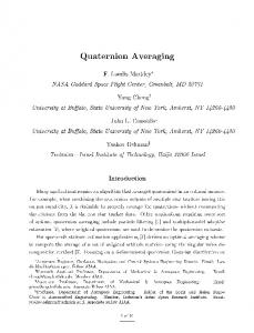
Figure 1: Rotation of a vector x, by an angle φ around the axis u. See text for details. Logarithm of unit quaternions It is immediate to see that, if kqk = 1, � � 0 uθ log q = log(cos θ + u sin θ) = log(e ) = uθ = , uθ
(34)
that is, the logarithm of a unit quaternion is a pure quaternion. Logarithm of general quaternions By extension, if q is a general quaternion, � � q q log kqk log q = log(kqk ) = log kqk + log = log kqk + uθ = . uθ kqk kqk
1.4 1.4.1
(35)
Rotations and cross-relations The 3D vector rotation formula
We illustrate in Fig. 1 the rotation, following a right-hand rule, of a general 3D vector x by an angle φ around the axis defined by the unit vector u. This is accomplished by decomposing the vector x into a part x|| parallel to u and a part x⊥ orthogonal to u, x|| = u (kxk cos α) = u u> x x⊥ = x − x|| = x − u u> x ,
(36) (37)
so that x = x|| +x⊥ . The parallel part does not rotate, and the orthogonal part experiences a planar rotation in the plane normal to u, that is, if we create an orthogonal base {e1 , e2 } of this plane with e1 = x⊥ e2 = u×x⊥ = u×x ,
(38) (39)
satisfying ke1 k = ke2 k, then x⊥ = e1 ·1 + e2 ·0, and the rotated orthogonal component is, x0⊥ = e1 cos φ + e2 sin φ = x⊥ cos φ + (u×x) sin φ ,
(40)
yielding the expression of the rotated vector, x0 = x|| + x0⊥ , which is known as the vector rotation formula, x0 = x|| + x⊥ cos φ + (u × x) sin φ . 7
(41)
1.4.2
Quaternion and rotation vector
Given the rotation vector v = φu, representing a right-handed rotation of φ rad around the axis given by the unit vector u = ux i + uy j + uz k, we build the unit quaternion q = ev/2 , which can be developed using an extension of the Euler formula (see (31)), � � φ φ cos(φ/2) . q = cos + (ux i + uy j + uz k) sin = u sin(φ/2) 2 2
(42)
(43)
We call this the rotation vector to quaternion conversion, denoted by q = q{v}. Conversely, using the 4-quadrant version of arctan(y, x) we have φ = 2 arctan(kqv k , qw ) u = qv / kqv k .
(44) (45)
Rotating a vector x by φ around u is performed with the double quaternion product, x0 = q ⊗ x ⊗ q∗ , where the vector x has been written in quaternion form, that is, � � 0 x = xi + yj + zk = . x
(46)
(47)
To see it, we use (10), (43), and basic vector and trigonometric identities, to develop the product (46) as follows, � � � � � � � � 0 cos φ2 0 cos φ2 ⊗ ⊗ , (48a) = x x0 u sin φ2 −u sin φ2 φ φ φ φ + (u ⊗ x − x ⊗ u) sin cos − u ⊗ x ⊗ u sin2 2 2 2 2 φ φ φ φ x cos2 + 2(u × x) sin cos − (x(u> u) − 2u(u> x)) sin2 2 2 2 2 φ φ φ φ φ x(cos2 − sin2 ) + (u × x)(2 sin cos ) + u(u> x)(2 sin2 ) 2 2 2 2 2 x cos φ + (u × x) sin φ + u(u> x)(1 − cos φ) (x − u u> x) cos φ + (u × x) sin φ + u u> x x⊥ cos φ + (u × x) sin φ + x|| ,
x0 = x cos2 = = = = =
which is precisely the vector rotation formula (41).
8
(48b)
1.4.3
Rotation matrix and rotation vector
The rotation matrix is also defined from the rotation vector v = φu, R = e[v]× ,
(49)
which we denote R = R{v}. The cross-product matrix, 0 −vz vy 0 −vx , [v]× , vz −vy vx 0
(50)
is a skew-symmetric matrix, [v]> × = − [v]× , left-hand-equivalent to the cross product, i.e., [v]× w = v×w ,
∀ v, w ∈ R3 .
(51)
When applied to unit vectors, u, the matrix [u]× satisfies [u]2× = uu> − I
[u]3×
(52)
= − [u]× ,
(53)
and thus all powers of [u]× can be expressed in terms of [u]× and [u]2× in a cyclic pattern, [u]4× = − [u]2×
,
[u]5× = [u]×
,
[u]6× = [u]2×
,
[u]7× = − [u]×
,
··· .
(54)
Now, writing the Taylor expansion of (49) with v = φu, 1 1 eφ[u]× = I + φ [u]× + φ2 [u]2× + φ3 [u]3× + . . . 2 3
(55)
grouping in terms of [u]× and [u]2× , and identifying in them, respectively, the series of sin φ and cos φ, leads to a closed form to obtain the rotation matrix from the rotation vector, the so called Rodrigues rotation formula, R = I + sin φ [u]× + (1 − cos φ) [u]2× .
(56)
Rotating a vector x by φ around u is performed with the linear product x0 = R x ,
(57)
as can be shown by developing (57), using (56) and (51–52), in a way akin to the last steps of (48), to obtain the vector rotation formula (41).
9
1.4.4
Rotation matrix and quaternion
Unit quaternions act as rotation operators in a way somewhat similar to rotation matrices, x0 = q ⊗ x ⊗ q∗ ,
x0 = R x .
Here, we used the bar notation x to indicate that the vector x in the left expression is expressed in quaternion form (47), thus differentiating it from that on the right. However, this circumstance is mostly unambiguous and can be derived from the context, and especially by the presence of the quaternion product ⊗. In what is to follow, we are omitting this bar and writing simply, x0 = q ⊗ x ⊗ q∗ , which allows us to abuse of the notation and write3 , q ⊗ x ⊗ q∗ = R x . (58) As both sides of this identity are linear in x, an expression of the rotation matrix equivalent to the quaternion is found by developing the left hand side and identifying terms on the right, yielding 2 2(qx qz + qw qy ) qw + qx2 − qy2 − qz2 2(qx qy − qw qz ) (59) R = 2(qx qy + qw qz ) qw2 − qx2 + qy2 − qz2 2(qy qz − qw qx ) , 2 2 2 2 2(qx qz − qw qy ) 2(qy qz + qw qx ) qw − qx − qy + qz denoted throughout this document by R = R{q}. The rotation matrix R has the following properties with respect to the quaternion, R{[1, 0, 0, 0]> } R{−q} R{q∗ } R{q1 ⊗ q2 }
= = = =
I R{q} R{q}> R{q1 }R{q2 } ,
(60) (61) (62) (63)
where we observe that: (60) the identity quaternion encodes the null rotation; (61) a quaternion and its negative encode the same rotation; (62) the conjugate quaternion encodes the inverse rotation; and (63) the quaternion product composes consecutive rotations in the same order as rotation matrices do. The matrix form of the quaternion product (14–15) provides us with an alternative formula for the rotation matrix, since � � � � 0 0 ∗ − ∗ + q ⊗ x ⊗ q = Q (q ) Q (q) = , (64) x Rx which leads after some easy developments to > R = (qw2 − q> v qv ) I + 2 qv qv + 2 [qv ]× . 3
(65)
� � � � 0 0 ∗ The proper expressions would be, q ⊗ x ⊗ q = Rx , or q ⊗ ⊗q = . See Section 1.2. x Rx ∗
10
1.5
Quaternion conventions. My choice.
There are several ways to determine the quaternion. They are basically related to four binary choices: • The order of its elements — real part first or last: � � � � qw q q= vs. q= v . qv qw
(66)
• The multiplication formula — definition of the quaternion algebra: ij = −ji = k
vs.
ji = −ij = k ,
(67a)
which correspond to different handedness, respectively: right-handed
vs.
left-handed.
(67b)
• The function of the rotation operator — rotating frames or rotating vectors: Passive
vs.
Active.
(68)
• In the passive case, the direction of the operation — local-to-global or global-to-local: xglobal = q ⊗ xlocal ⊗ q∗
vs.
xlocal = q ⊗ xglobal ⊗ q∗
(69)
This variety of choices leads to 12 different combinations. Historical developments have favored some conventions over others (Chou, 1992; Yazell, 2009). Today, in the available literature, we find many quaternion flavors such as the Hamilton, the STS4 , the JPL5 , the ISS6 , the ESA7 , the Engineering, the Robotics, and possibly a lot more denominations. Many of these forms might be identical, others not, but this fact is rarely explicitly stated, and many works simply lack a sufficient description of their quaternion with regard to the four choices above. The two most commonly used conventions, which are also the best documented, are Hamilton (the options on the left in (66–69)) and JPL (the options on the right, with the exception of (68)). Table 1 shows a summary of their characteristics. JPL is mostly used in the aerospace domain, while Hamilton is more common to other engineering areas such as robotics —though this should not be taken as a rule. My choice is to take the Hamilton convention, which is right-handed and coincides with many software libraries of widespread use in robotics, such as Eigen, ROS, Google Ceres, and with a vast amount of literature on Kalman filtering for attitude estimation using 4
Space Transportation System, commonly known as NASA’s Space Shuttle. Jet Propulsion Laboratory. 6 International Space Station. 7 European Space Agency. 5
11
Table 1: Hamilton vs. JPL quaternion conventions with respect to the 4 binary choices
1 2 3
Quaternion type
Hamilton
JPL
Components order
(qw , qv )
(qv , qw )
ij = k
ij = −k
Algebra Handedness
Right-handed
Left-handed
Passive
Passive
Local-to-Global
Global-to-Local
Function Right-to-left products mean
4 Default notation, q Default operation
q , qGL xG = q ⊗ xL ⊗ q
q , qLG ∗
xL = q ⊗ xG ⊗ q∗
IMUs (Chou, 1992; Kuipers, 1999; Pini´es et al., 2007; Roussillon et al., 2011; Martinelli, 2012, and many others). The JPL convention is possibly less commonly used, at least in the robotics field. It is extensively described in (Trawny and Roumeliotis, 2005), a reference work that has an aim and scope very close to the present one, but that concentrates exclusively in the JPL convention. The JPL quaternion is used in the JPL literature (obviously) and in key papers by Li, Mourikis, Roumeliotis, and colleagues (see e.g. (Li and Mourikis, 2012; Li et al., 2014)), which draw from Trawny and Roumeliotis’ document. These works are a primary source of inspiration when dealing with visual-inertial odometry and SLAM —which is what we do. In the rest of this section we analyze these two quaternion conventions with a little more depth. 1.5.1
Order of the quaternion components
Though not the most fundamental, the most salient difference between Hamilton and JPL quaternions is in the order of the components, with the scalar part being either in first (Hamilton) or last (JPL) position. The implications of such change are quite obvious and should not represent a great challenge of interpretation. In fact, some works with the quaternion’s real component at the end (e.g., the C++ library Eigen) are still considered as using the Hamilton notation, as long as the other three aspects are maintained. We have used the subscripts (w, x, y, z) for the quaternion components for increased clarity, instead of the other commonly used (0, 1, 2, 3). When changing the order, qw will always denote the real part, while it is not clear whether q0 would also do —in some occasions, one might find things such as q = (q1 , q2 , q3 , q0 ), with q0 real and last, but in the general case of q = (q0 , q1 , q2 , q3 ), the real part at the end would be q3 .8 When passing from one convention to the other, we must be careful of formulas involving full 4 × 4 or 8
See also footnote 1.
12
3 × 4 quaternion-related matrices, for their rows and/or columns need to be swapped. This is not difficult to do, but it might be difficult to detect and therefore prone to error. 1.5.2
Specification of the quaternion algebra
The Hamilton convention defines ij = k and therefore, i2 = j 2 = k 2 = ijk = −1 ,
ij = −ji = k ,
jk = −kj = i ,
ki = −ik = j ,
(70)
whereas the JPL convention defines ji = k and hence its quaternion algebra becomes, i2 = j 2 = k 2 = −ijk = −1 ,
−ij = ji = k ,
−jk = kj = i ,
−ki = ik = j .
(71)
Interestingly, these subtle sign changes preserve the basic properties of quaternions as rotation operators. However, they have the important consequence of changing the Cartesian space handedness (Shuster, 1993): Hamilton uses ij = k and is therefore righthanded; JPL uses ji = k and is left-handed (Trawny and Roumeliotis, 2005). These sign differences impact the respective formulas for rotation, composition, etc., in non-obvious ways. The formulas are thus not compatible, and we need to make a clear choice from the very start. 1.5.3
Function of the rotation operator
We have seen how to rotate vectors in 3D. This is referred to in (Shuster, 1993) as the Active interpretation, because operators (this affects all rotation operators) actively rotate vectors, x0 = qactive ⊗ x ⊗ q∗active , x0 = Ractive x . Another way of seeing the effect of q and R over a vector x is to consider that the vector is steady but it is us who have rotated our point of view by an amount specified by q or R. This is called here frame transformation and it is referred to in (Shuster, 1993) as the Passive interpretation, because vectors do not move, xB = qpassive ⊗ xA ⊗ q∗passive ,
xB = Rpassive xA ,
(72)
where A and B are two Cartesian frames, and xA and xB are expressions of the same vector x in these frames. See further down for explanations and proper notations. The active and passive interpretations are governed by operators inverse of each other, that is, qactive = q∗passive , Ractive = R> passive . Both Hamilton and JPL use the passive convention.
13
Direction cosine matrix As a final remark, we add that a few authors understand the passive operator as not being a rotation operator, but rather an orientation specification, named the direction cosine matrix, cxx cxy czx C = cxy cyy czy (73) cxz cyz czz where each component cij is the cosinus of the angle between the axis i in the local frame and the axis j in the global frame. We have the identity, C ≡ Rpassive 1.5.4
(74)
Direction of the rotation operator
In the passive case, a second source of interpretation is related to the direction in which the rotation matrix and quaternion operate, either converting from local to global frames, or from global to local. Given two Cartesian frames G and L, we identify G and L as being the local and global frames, “global” and “local” being relative definitions, i.e., G is global with respect to L, and L is local with respect to G. We specify qGL and RGL as being the quaternion and rotation matrix transforming vectors from frame L to frame G, in the sense that a vector xL in frame L is expressed in frame G with the quaternion- and matrix- products xG = qGL ⊗ xL ⊗ q∗GL ,
xG = RGL xL .
(75)
xL = RLG xG ,
(76)
The opposite conversion is done with xL = qLG ⊗ xG ⊗ q∗LG , with qLG = q∗GL ,
RLG = R> GL .
(77)
Hamilton uses local-to-global as the default specification of a frame L expressed in frame G, qHamilton , q[with respect to][of ] = q[to][f rom] = qGL , (78) while JPL uses the opposite, global-to-local conversion, qJP L , q[of ][with
respect to]
= q[to][f rom] = qLG .
(79)
Notice that qJP L ∼ qLG,passive = q∗LG,active = qGL,active = q∗GL,passive ∼ q∗Hamilton ,
(80)
which is not particularly useful, but illustrates how easy it is to get confused when mixing conventions. Moreover, notice that because of the quaternion algebra differences between Hamilton and JPL (which imply different handedness), it is not generally correct to assume from (80) that qJP L = q∗Hamilton (this is why we used the sign ∼ in the expression above). 14
1.5.5
Notation
An often underestimated source of confusion when dealing with quaternion algebra is related to notation. We believe notation should be clear, lightweight and unambiguous. Of course, this applies not only to quaternions and rotation matrices, but also to the points and vectors manipulated by these. A good notation requires considering many conflicting aspects: • Clearly distinguish scalars, vectors, matrices and functions with different font styles. ˜ , hats q ˆ , bars q ¯ , q, and other accents, as much • Avoid tiny elements such as tildes q as possible. • Avoid making extensive use of unusual Greek symbols. If we cannot tell a symbol name, then we cannot read a formula. What is Ξ? And Υ? • Avoid certain combinations of subscripts and superscripts on the left and right hand sides, especially when they appear in multiple levels, e.g., Ci xFj . They produce formulas such as i uj =
Ci x F Ci z F
j
(which is the pinhole camera model) that are difficult
j
to read because the main variables, x and z, are not salient enough. • Make composition of chains obviously and unambiguously readable. For example, B the rotation matrix RB A or the quaternion A q are ambiguous because we do not know if they transform “A to B” or “B to A”. • Provide easy 1:1 translation to readable programming code. This last point becomes increasingly important as most of the works we produce are meant to be translated into algorithms. Our notation derives from the following rules, 1. Scalars are a, x, ω; vectors are a, x, ω, matrices are A, X, Ω; functions are f (), g(). ˆ , to signify the mean of the Kalman filter Gaussian 2. The only accent we use is the hat, x estimate. Error-state values are noted δx. 3. The general translation specification t needs 3 decorations: a translation from point B / to point C / expressed in frame A, t[expressed
in],[initial point][end point]
.
(81)
This produces forms such as tA,BC . We define two convenient simplifications: • When tA,BC refers to a point p = C, we consider its origin at the origin of the reference frame, i.e., B = O, giving pA , tA,OC . 15
(82)
• When tA,BC refers to a free vector v = BC, we may simply write vA , tA,BC .
(83)
In both cases we keep the reference frame A where the point or vector is expressed in. In case of no ambiguity, when this frame is the world frame W of our application we allow us to drop this decoration too. For example, the position P of the robot in the world frame may be denoted simply by p, p , pW = tW,OP .
(84)
4. The general orientation specification, q or R, requires 2 decorations: a transformation from frame B / to frame A, or equivalently, the orientation of frame B / with respect to frame A, R[to][f rom] ≡ R[with respect to][of ] . (85) This produces forms such as RAB that lead unambiguously to xA = RAB xB . Stacked or composed transforms produce chains such as xA = qAB ⊗ qBC ⊗ xC ⊗ q∗BC ⊗ q∗AB ,
xA = RAB RBC xC .
(86)
which are readable and not prone to error. Notice how each of the two frame identifiers is always at the side of the entity nearby (though in the quaternion transform above, this only applies to the quaternions chain on the left of the vector, the ones that are not conjugated). This allows us to easily construct and/or identify frame composition chains with absolutely no ambiguity. In cases where there is no ambiguity, the world frame W and the frame of the main moving body B may be omitted, yielding q , qWB ,
R , RWB .
(87)
This, and the simplifications for points and vectors (82–84) above, lead to x = q ⊗ xB ⊗ q∗ ,
x = R xB ,
(88)
which are very light and easy to read. 5. We use only right-hand subscripts for frame decorations. This way, translating formulas into code and vice-versa becomes straightforward. In the code, the first letter before the first underscore is always the physical magnitude. For example, these formula and code are equivalent, xA = RAB * RBC * xC.
xA = RAB RBC xC ,
16
(89)
1.6
Frame composition
As we have briefly seen in (86), quaternion composition is done similarly to rotation matrices, i.e., with appropriate quaternion- and matrix- products, and in the same order, qAC = qAB ⊗ qBC ,
RAC = RAB RBC .
(90)
The Hamilton, local-to-global convention adopted here establishes that compositions go from local to global when moving towards the left of the composition chain, or from global to local when moving right. This means that qBC and RBC are specifications of a frame C that is local with respect to frame B. We illustrate the composed transform using the quaternion, xA = = = = =
1.7 1.7.1
qAB ⊗ xB ⊗ q∗AB qAB ⊗ (qBC ⊗ xC ⊗ q∗BC ) ⊗ q∗AB (qAB ⊗ qBC ) ⊗ xC ⊗ (q∗BC ⊗ q∗AB ) (qAB ⊗ qBC ) ⊗ xC ⊗ (qAB ⊗ qBC )∗ qAC ⊗ xC ⊗ q∗AC .
Perturbations and time-derivatives Local perturbations
˜ may be expressed as the composition of the unperturbed orienA perturbed orientation q tation q with a small local perturbation ∆qL . Because of the Hamilton convention, this local perturbation appears at the right hand side of the composition product —we give also the matrix equivalent for comparison, ˜ = R ∆RL . R
˜ = q ⊗ ∆qL , q
(91)
If the perturbation angle ∆θL , ∆φ·u is small then the perturbation quaternion and rotation matrix can be approximated by the Taylor expansions of (43) and (49) up to the linear terms, � � 1 + O(k∆θL k2 ) , ∆RL = I + [∆θL ]× + O(k∆θL k2 ). (92) ∆qL = 1 ∆θ L 2 With this we can easily develop expressions for the time-derivatives. Just consider q = q(t) ˜ = q(t + ∆t) as the perturbed state, and apply the definition of the as the original state, q derivative dq(t) q(t + ∆t) − q(t) , lim , (93) ∆t→0 dt ∆t to the above, with dθL (t) ∆θL ωL (t) , , lim , (94) ∆t→0 ∆t dt 17
which, being ∆θL a local angular perturbation, corresponds to the angular rates vector in the body frame. The development of the time-derivative of the quaternion follows (an analogous reasoning would be used for the rotation matrix) q(t + ∆t) − q(t) ∆t→0 ∆t q ⊗ ∆qL − q lim ∆t→0 ∆t �� � � �� 1 1 q⊗ − ∆θL /2 0 lim ∆t→0 ∆t� � 0 q⊗ ∆θL /2 lim ∆t→0 ∆t � � 1 0 q⊗ . ω 2 L
q˙ , lim =
=
= =
(95)
Defining 0 −ω −ω −ω x y z � � ωx 0 −ω > 0 ωz −ωy − , Ω(ω) , Q (ω) = = ωy −ωz ω − [ω]× 0 ωx ωz ωy −ωx 0
(96)
we get from (95) and (14) (we give also its matrix equivalent) 1 1 q˙ = Ω(ωL ) q = q ⊗ ωL , 2 2 1.7.2
˙ = R [ωL ] . R ×
(97)
Global perturbations
It is possible and indeed interesting to consider globally-defined perturbations, and likewise for the related derivatives. Global perturbations appear at the left hand side of the composition product, namely, ˜ = ∆RG R . R
˜ = ∆qG ⊗ q , q
(98)
The associated time-derivatives follow from a development analogous to (95), which results in 1 ˙ = [ωG ] R , q˙ = ωG ⊗ q , R (99) × 2 where
dθG (t) dt is the angular rates vector expressed in the global frame. ωG (t) ,
18
(100)
1.7.3
Global-to-local relations
It is worth noticing the following relation between local and global angular rates, 1 1 ωG ⊗ q = q˙ = q ⊗ ωL . 2 2
(101)
Then, post-multiplying by the conjugate quaternion we have ωG = q ⊗ ωL ⊗ q∗ = R ωL .
(102)
Likewise, considering that ∆θR ≈ ω∆t for small ∆t, we have that ∆θG = q ⊗ ∆θL ⊗ q∗ = R ∆θL .
(103)
That is, we can transform angular rates vectors ω and small angular perturbations ∆θ via frame transformation, using the quaternion or the rotation matrix, as if they were regular vectors. The same can be seen by posing ∆θ = u∆θ and noticing that the rotation axis vector u transforms normally, with uG = q ⊗ uL ⊗ q∗ = R uL . 1.7.4
(104)
Time-derivative of the quaternion product
We use the regular formula for the derivative of the product, ˙ q2 ) = q˙1 ⊗ q2 + q1 ⊗ q˙2 , (q1 ⊗
˙ 1 R2 + R1 R ˙2, (R1˙R2 ) = R
(105)
but noticing that, since the products are non commutative, we need to respect the order of the operands strictly. This means that (q˙2 ) = 6 2 q ⊗ q˙ , but rather (q˙2 ) = q˙ ⊗ q + q ⊗ q˙ . 1.7.5
(106)
Other useful expressions with the derivative
We can derive an expression for the local rotation rate ωL = 2 q∗ ⊗ q˙ ,
˙ . [ωL ]× = R> R
(107)
˙ R> . [ωG ]× = R
(108)
and the global rotation rate, ωG = 2 q˙ ⊗ q∗ ,
19
Figure 2: Angular velocity approximations for the integral: Red: true velocity. Blue: zeroth order approximations (bottom to top: forward, midward and backward). Green: first order approximation.
1.8
Time-integration of rotation rates
Accumulating rotation over time in quaternion form is done by integrating the differential equation appropriate to the rotation rate definition, that is, (97) for a local rotation rate definition, and (99) for a global one. In the cases we are interested in, the angular rates are measured by local sensors, thus providing local measurements ω(tn ) at discrete times tn = n∆t. We concentrate here on this case only, for which we reproduce the differential equation (97), 1 ˙ (109) q(t) = q(t) ⊗ ω(t) . 2 We develop zeroth- and first- order integration methods (Fig. 2), all based on the Taylor series of q(tn + ∆t) around the time t = tn . We note q , q(t) and qn , q(tn ), and the same for ω. The Taylor series reads, qn+1 = qn + q˙ n ∆t +
1 ... 1 .... 1 q n ∆t4 + · · · . ¨ n ∆t2 + q n ∆t3 + q 2! 3! 4!
(110)
The successive derivatives of qn above are easily obtained by repeatedly applying the ¨ = 0. We obtain expression of the quaternion derivative, (109), with ω 1 qn ωn 2 1 1 ¨ n = 2 qn ωn2 + qn ω˙ q 2 2 ... 1 1 1 3 qn = ˙ q ω + q ω ω + q ωn ω˙ n n n n 23 4 2 1 qn(i ≥ 4) = i qn ωni + · · · , 2 q˙ n =
(111a) (111b) (111c) (111d)
where we have omitted the ⊗ signs for economy of notation, that is, all products and the powers of ω must be interpreted in terms of the quaternion product.
20
1.8.1
Zeroth order integration
Forward integration In the case where the angular rate ωn is held constant over the period ∆t = tn+1 − tn , we have ω˙ = 0 and the Taylor series can be written as, � � �2 1 � 1 �3 1 � 1 �4 1 1 �1 qn+1 = qn ⊗ 1 + ωn ∆t + ωn ∆t + ωn ∆t + ωn ∆t + · · · , 2 2! 2 3! 2 4! 2 (112) ωn ∆t/2 in which we identify the Taylor series of the exponential e . From (42–43), this exponential corresponds to the quaternion representing the incremental rotation ∆θ = ωn ∆t, � � cos(kωk ∆t/2) ω∆t/2 , e = q{ω∆t} = ω sin(kωk ∆t/2) kωk therefore, qn+1 = qn ⊗ q{ωn ∆t} .
(113)
Backward integration We can also consider that the constant velocity over the period ∆t corresponds to ωn+1 , the velocity measured at the end of the period. This can be developed in an similar manner with a Taylor expansion of qn around tn+1 , leading to qn+1 = qn ⊗ q{ωn+1 ∆t} .
(114)
Midward integration Similarly, if the velocity is considered constant at the median rate over the period ∆t (which is not necessary the velocity at the midpoint of the period), ¯ = ω
ωn+1 + ωn , 2
(115)
we have, ¯ qn+1 ≈ qn ⊗ q{ ω∆t} . 1.8.2
(116)
First order integration
The angular rate ω(t) is now linear with time. Its first derivative is constant, and all higher ones are zero, ωn+1 − ωn ∆t ... ¨ = ω = ··· = 0 . ω ω˙ =
(117) (118)
¯ in terms of ωn and ω, ˙ We can write the median rate ω ¯ = ωn + ω 21
1 ˙ ω∆t , 2
(119)
and derive the expression of the powers of ωn appearing in the quaternion derivatives ¯ and ω, ˙ (111), in terms of the more convenient ω 1 ˙ ω∆t 2 1 1 1 ¯2 − ω ¯ ω∆t ˙ ¯ ωn2 = ω − ω˙ ω∆t + ω˙ 2 ∆t2 2 2 4 3 3 1 ¯3 − ω ¯ 2 ω∆t ˙ ¯ ω˙ 2 ∆t2 + ω˙ 3 ∆t3 ωn3 = ω + ω 2 4 8 4 4 ¯ + ··· . ωn = ω ¯− ωn = ω
Injecting them in the quaternion derivatives, and substituting in the Taylor series (110), we have after proper reordering, ! � �2 � �3 1 1 1 1 1 ¯ ¯ ¯ qn+1 = q 1 + ω∆t + ω∆t + ω∆t + ··· (121a) 2 2! 2 3! 2 � � 1 1 + q − ω˙ + ω˙ ∆t2 (121b) 4 4 � � 1 1 1 1 ¯ ω˙ − ¯+ ¯+ ¯ ω˙ ∆t3 ω˙ ω ω˙ ω ω (121c) +q − ω 16 16 24 12 � � + q · · · ∆t4 + · · · , (121d) ¯ where in (121a) we recognize the Taylor series of the exponential e ω∆t/2 , (121b) vanishes, and (121d) represents terms of high multiplicity that we are going to neglect. From (42– ¯ ¯ 43), we have e ω∆t/2 = q{ ω∆t}, the quaternion representing the incremental rotation ¯ ∆θ = ω∆t, now using the average rotation rate over the period ∆t. This yields after simplification (we recover now the normal ⊗ notation),
¯ qn+1 = qn ⊗ q{ ω∆t} +
∆t3 ¯ ⊗ ω˙ − ω˙ ⊗ ω) ¯ + ··· . qn ⊗ ( ω 48
(122)
¯ by their definitions (117) and (115) we get, Substituting ω˙ and ω ¯ qn+1 = qn ⊗ q{ ω∆t} +
∆t2 qn ⊗ ( ωn ⊗ ωn+1 − ωn+1 ⊗ ωn ) + · · · , 48
(123)
which is a result equivalent to (Trawny and Roumeliotis, 2005)’s, but using the Hamilton convention, and the quaternion product form instead of the matrix product form. Finally, since av ⊗ bv − bv ⊗ av = 2 av ×bv , see (28), we have the alternative form, qn+1
� � ∆t2 0 ¯ ≈ qn ⊗ q{ ω∆t} + qn ⊗ . ωn × ωn+1 24 22
(124)
In this expression, the first term of the sum is the midward zeroth order integrator (116). The second term is a second-order correction that vanishes when ωn and ωn+1 are collinear,9 i.e., when the axis of rotation has not changed from tn to tn+1 . Given usual IMU sampling times ∆t ≤ 0.01s and the usual near-collinearity of ωn and ωn+1 , this term takes values of the order of 10−6 kωk2 , or easily smaller. Terms with higher multiplicities of ω∆t are even smaller and have been neglected.
2
Error-state kinematics for IMU-driven systems
2.1
Motivation
We wish to write the error-estate equations of the kinematics of an inertial system integrating accelerometer and gyrometer readings with bias and noise, using the Hamilton quaternion to represent the orientation in space or attitude. These readings come typically from an Inertial Measurement Unit (IMU). Integrating IMU readings leads to deadreckoning positioning systems, which drift with time. Avoiding drift is a matter of fusing this information with absolute position readings such as GPS or vision. The error-state Kalman filter (ESKF) is one of the tools we may use for this purpose. Within the Kalman filtering paradigm, these are the most remarkable assets of the ESKF: • The orientation error-state is minimal (i.e., it has the same number of parameters as degrees of freedom), avoiding issues related to over-parametrization (or redundancy) and the consequent risk of singularity of the involved covariances matrices, resulting typically from enforcing constraints. • The error-state system is always operating close to the origin, and therefore far from possible parameter singularities, gimbal lock issues, or the like, providing a guarantee that the linearization validity holds at all times. • The error-state is always small, meaning that all second-order products are negligible. This makes the computation of Jacobians very easy and fast. Some Jacobians may even be constant or equal to available state magnitudes. • The error dynamics are slow because all the large-signal dynamics have been integrated in the nominal-state. This means that we can apply KF corrections (which are the only means to observe the errors) at a lower rate than predictions.
2.2
The error-state Kalman filter explained
In error-state filter formulations, we speak of true-, nominal- and error-state values, the true-state being expressed as a suitable composition (linear sum, quaternion product or 9
Notice also from (123) that this term would always vanish if the quaternion product were commutative, which is not.
23
matrix product) of the nominal- and the error- states. The idea is to consider the nominalstate as large-signal (integrable in non-linear fashion) and the error-state as small signal (thus linearly integrable and suitable for linear-Gaussian filtering). The error-state filter can be explained as follows. On one side, high-frequency IMU data um is integrated into a nominal-state x. This nominal state does not take into account the noise terms w and other possible model imperfections. As a consequence, it will accumulate errors. These errors are collected in the error-state δx and estimated with the Error-State Kalman Filter (ESKF), this time incorporating all the noise and perturbations. The errorstate consists of small-signal magnitudes, and its evolution function is correctly defined by a (time-variant) linear dynamic system, with its dynamic, control and measurement matrices computed from the values of the nominal-state. In parallel with integration of the nominalstate, the ESKF predicts a Gaussian estimate of the error-state. It only predicts, because by now no other measurement is available to correct these estimates. The filter correction is performed at the arrival of information other than IMU (e.g. GPS, vision, etc.), which is able to render the errors observable and which happens generally at a much lower rate than the integration phase. This correction provides a posterior Gaussian estimate of the error-state. After this, the error-state’s mean is injected into the nominal-state, then reset to zero. The error-state’s covariances matrix is conveniently updated to reflect this reset. The system goes on like this forever.
2.3
System kinematics in continuous time
The definition of all the involved variables is summarized in Table 2. Two important decisions regarding conventions are worth mentioning: • The angular rates ω are defined locally with respect to the nominal quaternion. This allows us to use the gyrometer measurements ωm directly, as they provide bodyreferenced angular rates. • The angular error δθ is also defined locally with respect to the nominal orientation. This is not necessarily the optimal way to proceed, but it corresponds to the choice in most IMU-integration works —what we could call the classical approach. There exists evidence (Li and Mourikis, 2012) that a globally-defined angular error has better properties. This will be explored too in the present document, Section 4, but most of the developments, examples and algorithms here are based in this locallydefined angular error.
24
Table 2: All variables in the error-state Kalman filter. Magnitude
True
Nominal Error
Composition
Full state (1 )
xt
x
δx
xt = x ⊕ δx
Position
pt
p
δp
pt = p + δp
Velocity
vt
v
δv
vt = v + δv
Quaternion (2,3 )
qt
q
δq
Rotation matrix (2,3 )
Rt
R
δR
qt = q ⊗ δq
Angles vector
Measured
Noise
Rt = R δR " # 1 δq ≈ δθ/2
δθ
δR ≈ I + [δθ]×
Accelerometer bias
abt
ab
δab
abt = ab + δab
aw
Gyrometer bias
ωbt
ωb
δωb
ωbt = ωb + δωb
ωw
Gravity vector
gt
g
δg
gt = g + δg
Acceleration
at
am
an
Angular rate
ωt
ωm
ωn
(1 ) the symbol ⊕ indicates a generic composition
(2 ) indicates non-minimal representations
(3 ) see Table 3 for the composition formula in case of globally-defined angular errors 2.3.1
The true-state kinematics
The true kinematic equations are p˙ t = vt v˙ t = at 1 q˙t = qt ⊗ ωt 2 a˙ bt = aw ω˙ bt = ωw g˙ t = 0
25
(125a) (125b) (125c) (125d) (125e) (125f)
Here, the true acceleration at and angular rate ωt are obtained from an IMU in the form of noisy sensor readings am and ωm in body frame, namely10 am = R> t (at − gt ) + abt + an ωm = ωt + ωbt + ωn
(126) (127)
with Rt , R(qt ). With this, the true values can be isolated (this means that we have inverted the measurement equations), at = Rt (am − abt − an ) + gt ωt = ωm − ωbt − ωn .
(128) (129)
Substituting above yields the kinematic system p˙ t = vt v˙ t = Rt (am − abt − an ) + gt 1 q˙t = qt ⊗ (ωm − ωbt − ωn ) 2 a˙ bt = aw ω˙ bt = ωw g˙ t = 0
(130a) (130b) (130c) (130d) (130e) (130f)
which we may name x˙ t = ft (xt , u, w). This system has state xt , is governed by IMU noisy readings um , and is perturbed by white Gaussian noise w, all defined by pt vt � � � � qt a a − a m n (131) u= w= w . xt = abt ωw ωm − ωn ωbt gt It is to note in the above formulation that the gravity vector gt is going to be estimated by the filter. It has a constant evolution equation, (130f), as corresponds to a magnitude that is known to be constant. The system starts at a fixed and arbitrarily known initial orientation qt (t = 0) = q0 , which, being generally not in the horizontal plane, makes the initial gravity vector generally unknown. For simplicity it is usually taken q0 = (1, 0, 0, 0) and thus R0 = R{q0 } = I. We estimate gt expressed in frame q0 , and not qt expressed in a horizontal frame, so that the initial uncertainty in orientation is transferred to an initial uncertainty on the gravity direction. We do so to improve linearity: indeed, equation 10
It is common practice to neglect the Earth’s rotation rate ωE in (127), which would otherwise be ωm = ωt + R> t ωE + ωbt + ωn . This is in most cases unjustifiably complicated.
26
(130b) is now linear in g, which carries all the uncertainty, and the initial orientation q0 is known without uncertainty, so that q starts with no uncertainty. Once the gravity vector is estimated the horizontal plane can be recovered and, if desired, the whole state and recovered motion trajectories can be re-oriented to reflect the estimated horizontal. See (Lupton and Sukkarieh, 2009) for further justification. This is of course optional, and the reader is free to remove all equations related to graviy from the system and adopt a more classical approach of considering g , (0, 0, −9.8xx), with xx the appropriate decimal digits of the gravity vector on the site of the experiment, and an uncertain initial orientation q0 . 2.3.2
The nominal-state kinematics
The nominal-state kinematics corresponds to the modeled system without noises or perturbations, p˙ = v v˙ = R(am − ab ) + g 1 q˙ = q ⊗ (ωm − ωb ) 2 a˙ b = 0 ω˙ b = 0 g˙ = 0. 2.3.3
(132a) (132b) (132c) (132d) (132e) (132f)
The error-state kinematics
The goal is to determine the linearized dynamics of the error-state. For each state equation, we write its composition (in Table 2), solving for the error state and simplifying all second-order infinitesimals. We give here the full error-state dynamic system and proceed afterwards with comments and proofs. ˙ = δv δp ˙ = −R [am − ab ] δθ − Rδab + δg − Ran δv × ˙ = − [ωm − ωb ] δθ − δωb − ωn δθ × δa˙ b = aw ˙ b = ωw δω ˙ = 0. δg
(133a) (133b) (133c) (133d) (133e) (133f)
Equations (133a), (133d), (133e) and (133f), respectively of position, both biases, and gravity errors, are derived from linear equations and their error-state dynamics is trivial. As an example, consider the true and nominal position equations (130a) and (132a), their ˙ to obtain (133a). composition pt = p + δp from Table 2, and solve for δp Equations (133b) and (133c), of velocity and orientation errors, require some nontrivial manipulations of the non-linear equations (130b) and (130c) to obtain the linearized dynamics. Their proofs are developed in the following two sections. 27
˙ the dynamics Equation (133b): The linear velocity error. We wish to determine δv, of the velocity errors. We start with the following relations Rt = R(I + [δθ]× ) + O(kδθk2 ) v˙ = RaB + g,
(134) (135)
where (134) is the small-signal approximation of Rt , and in (135) we rewrote (132b) but introducing aB and δaB , defined as the large- and small-signal accelerations in body frame, aB , am − ab δaB , −δab − an
(136) (137)
so that we can write the true acceleration in inertial frame as a composition of large- and small-signal terms, at = Rt (aB + δaB ) + g + δg. (138) We proceed by writing the expression (130b) of v˙ t in two different forms (left and right developments), where the terms O(kδθk2 ) have been ignored, ˙ = v˙ t = R(I + [δθ] )(aB + δaB ) + g + δg v˙ + δv × ˙ = RaB + g + δv
= RaB + RδaB + R [δθ]× aB + R [δθ]× δaB + g + δg
This leads after removing RaB + g from left and right to ˙ = R(δaB + [δθ] aB ) + R [δθ] δaB + δg δv × ×
(139)
Eliminating the second order terms and reorganizing some cross-products (with [a]× b = − [b]× a), we get ˙ = R(δaB − [aB ] δθ) + δg, δv (140) × then, recalling (136) and (137), ˙ = R(− [am − ab ] δθ − δab − an ) + δg δv ×
(141)
which after proper rearranging leads to the dynamics of the linear velocity error, ˙ = −R [am − ab ] δθ − Rδab + δg − Ran . δv ×
(142)
To further clean up this expression, we can often times assume that the accelerometer noise is white, uncorrelated and isotropic11 , 2 E[an a> n ] = σa I,
E[an ] = 0 11
(143)
This assumption cannot be made in cases where the three XY Z accelerometers are not identical.
28
that is, the covariance ellipsoid is a sphere centered at the origin, which means that its mean and covariances matrix are invariant upon rotations (Proof: E[Ran ] = RE[an ] = 0 > = Rσa2 IR> = σa2 I). Then we can redefine the and E[(Ran )(Ran )> ] = RE[an a> n ]R accelerometer noise vector, with absolutely no consequences, according to an ← Ran
(144)
˙ = −R [am − ab ] δθ − Rδab + δg − an . δv ×
(145)
which gives
˙ the dynamics of Equation (133c): The orientation error. We wish to determine δθ, the angular errors. We start with the following relations 1 qt ⊗ ωt (146) 2 1 q˙ = q ⊗ ω, (147) 2 which are the true- and nominal- definitions of the quaternion derivatives. As we did with the acceleration, we group large- and small-signal terms in the angular rate for clarity, q˙t =
ω , ωm − ωb δω , −δωb − ωn ,
(148) (149)
so that ωt can be written with a nominal part and an error part, ωt = ω + δω.
(150)
We proceed by computing q˙t by two different means (left and right developments) 1 qt ⊗ ωt = q˙t = (q ⊗˙ δq) 2 1 q ⊗ δq ⊗ ωt = 2
˙ = q˙ ⊗ δq + q ⊗ δq 1 ˙ = q ⊗ ω ⊗ δq + q ⊗ δq 2
˙ we obtain simplifying the leading q and isolating δq � � 0 ˙ ˙ = 2δq = δq ⊗ ωt − ω ⊗ δq δθ = Q− (ωt )δq − Q+ (ω)δq � �� � 0 −(ωt − ω)> 1 = + O(kδθk2 ) (ωt − ω) − [ωt + ω]× δθ/2 � �� � 0 −δω > 1 = + O(kδθk2 ) δω − [2ω + δω]× δθ/2 29
(151)
which results in one scalar- and one vector- equalities 0 = δω > δθ + O(|δθ|2 ) (152) 1 ˙ = δω − [ω] δθ − [δω] δθ + O(kδθk2 ). δθ (153) × × 2 The first equation leads to δω > δθ = O(kδθk2 ), which is formed by second-order infinitesimals, not very useful. The second equation yields, after neglecting all second-order terms, ˙ = − [ω] δθ + δω δθ (154) ×
and finally, recalling (148) and (149), we get the linearized dynamics of the angular error, ˙ = − [ωm − ωb ] δθ − δωb − ωn . δθ ×
2.4
(155)
System kinematics in discrete time
The differential equations above need to be integrated into differences equations to account for discrete time intervals ∆t > 0. The integration methods may vary. In some cases, one will be able to use exact closed-form solutions. In other cases, numerical integration of varying degree of accuracy may be employed. Please refer to the Appendices for pertinent details on integration methods. Integration needs to be done for the following sub-systems: 1. The nominal state. 2. The error-state. (a) The deterministic part: state dynamics and control. (b) The stochastic part: noise and perturbations. 2.4.1
The nominal state kinematics
We can write the differences equations of the nominal-state as 1 p ← p + v ∆t + (R(am − ab ) + g) ∆t2 2 v ← v + (R(am − ab ) + g) ∆t q ← q ⊗ q{(ωm − ωb ) ∆t} ab ← ab ωb ← ωb g←g,
(156a) (156b) (156c) (156d) (156e) (156f)
where x ← f (x, •) stands for a time update of the type xk+1 = f (xk , •k ), R , R{q} is the rotation matrix associated to the current nominal orientation q, and q{v} is the quaternion associated to the rotation v, according to (43). We can also use more precise integration, please see the Appendices for more information. 30
2.4.2
The error-state kinematics
The deterministic part is integrated normally (in this case we follow the methods in App. C.2), and the integration of the stochastic part results in random impulses (see App. E), thus, δp ← δp + δv ∆t δv ← δv + (−R [am − ab ]× δθ − Rδab + δg)∆t + vi
δθ δab δωb δg
← ← ← ←
R> {(ωm − ωb )∆t}δθ − δωb ∆t + θi δab + ai δωb + ωi δg .
(157a) (157b) (157c) (157d) (157e) (157f)
Here, vi , θi , ai and ωi are the random impulses applied to the velocity, orientation and bias estimates, modeled by white Gaussian processes. Their mean is zero, and their covariances matrices are obtained by integrating the covariances of an , ωn , aw and ωw over the step time ∆t (see App. E), (158) = σa˜2n ∆t2 I [m2 /s2 ] 2 2 2 = σω˜ n ∆t I [rad ] (159) [m2 /s4 ] (160) = σa2w ∆tI 2 2 2 (161) = σωw ∆tI [rad /s ] √ √ where σa˜n [m/s2 ], σω˜ n [rad/s], σaw [m/s2 s] and σωw [rad/s s] are to be determined from the information in the IMU datasheet, or from experimental measurements. Vi Θi Ai Ωi
2.4.3
The error-state Jacobian and perturbation matrices
The Jacobians are obtained by simple inspection of the error-state differences equations in the previous section. To write these equations in compact form, we consider the nominal state vector x, the error state vector δx, the input vector um , and the perturbation impulses vector i, as follows (see App. E.1 for details and justifications), p δp v δv vi � � q δθ a θi m x= , i= (162) ab , δx = δab , um = ωm ai ωb δωb ωi g δg The error-state system is now δx ← f (x, δx, um , i) = Fx (x, um )·δx + Fi ·i, 31
(163)
The ESKF prediction equations are written: ˆ ← Fx (x, um )· δx ˆ δx > P ← Fx PFx + Fi Qi F> i ,
(164) (165)
ˆ P}12 ; Fx and Fi are the Jacobians of f () with respect to the error and where δx ∼ N {δx, perturbation vectors; and Qi is the covariances matrix of the perturbation impulses. The expressions of the Jacobian and covariances matrices above are detailed below. All state-related values appearing herein are extracted directly from the nominal state. I I∆t 0 0 0 0 0 I −R [am − ab ]× ∆t −R∆t 0 I∆t 0 0 R> {(ωm − ωb )∆t} ∂f 0 −I∆t 0 Fx = = (166) 0 I 0 0 ∂δx x,um 0 0 0 0 0 0 I 0 0 0 0 0 0 I
∂f Fi = ∂i x,um
0 I 0 = 0 0 0
0 0 I 0 0 0
0 0 0 I 0 0
0 0 0 0 I 0
,
Vi 0 0 0 0 Θi 0 0 Qi = 0 0 Ai 0 . 0 0 0 Ωi
(167)
Please note particularly that Fx is the system’s transition matrix, which can be approximated to different levels of precision in a number of ways. We showed here one of its simplest forms (the Euler form). Se Appendices B to D for further reference. Please note also that, being the mean of the error δx initialized to zero, the linear equation (164) always returns zero. You should of course skip line (164) in your code. I recommend that you write it, though, but that you comment it out so that you are sure you did not forget anything. And please note, finally, that you should NOT skip the covariance prediction (165)!! In effect, the term Fi Qi F> i is not null and therefore this covariance grows continuously – as it must be in any prediction step.
3
Fusing IMU with complementary sensory data
At the arrival of other kind of information than IMU, such as GPS or vision, we proceed to correct the ESKF. In a well-designed system, this should render the IMU biases observable and allow the ESKF to correctly estimate them. There are a myriad of possibilities, the most popular ones being GPS + IMU, monocular vision + IMU, and stereo vision + 12
x ∼ N {µ, Σ} means that x is a Gaussian random variable with mean and covariances matrix specified by µ and Σ.
32
IMU. In recent years, the combination of visual sensors with IMU has attracted a lot of attention, and thus generated a lot of scientific activity. These vision + IMU setups are very interesting for use in GPS-denied environments, and can be implemented on mobile devices (typically smart phones), but also on UAVs and other small, agile platforms. While the IMU information has served so far to make predictions to the ESKF, this other information is used to correct the filter. The correction consists of three steps: 1. observation of the error-state via filter correction, 2. injection of the observed errors into the nominal state, and 3. reset of the error-state. These steps are developed in the following sections.
3.1
Observation of the error state via filter correction
Suppose as usual that we have a sensor that delivers information that depends on the state, such as y = h(xt ) + v , (168) where h() is a general nonlinear function of the system state (the true state), and v is a white Gaussian noise with covariance V, v ∼ N {0, V} .
(169)
Our filter is estimating the error state, and therefore the filter correction equations13 , K = PH> (HPH> + V)−1 ˆ ← K(y − h(ˆ δx xt )) P ← (I − KH)P
(170) (171) (172)
require the Jacobian matrix H to be defined with respect to the error state δx, and evalˆ As the error state mean is zero at this ˆ t = x ⊕ δx. uated at the best true-state estimate x ˆ t = x and we can use the nominal error x stage (we have not observed it yet), we have x as the evaluation point, leading to ∂h . (173) H≡ ∂δxt x 13
We give the simplest form of the covariance update, P ← (I−KH)P. This form is known to have poor numerical stability, as its outcome is not guaranteed to be symmetric nor positive definite. The reader is free to use more stable forms such as 1) the symmetric form P ← P − K(HPH> + V)K> and 2) the symmetric and positive Joseph form P ← (I − KH)P(I − KH)> + KVK> .
33
3.1.1
Jacobian computation for the filter correction
The Jacobian above might be computed in a number of ways. The most illustrative one is by making use of the chain rule, ∂h ∂h ∂xt H, = = Hx Xδx . (174) ∂δxt x ∂xt x ∂δx x ∂h Here, Hx , ∂x is the standard Jacobian of h() with respect to its own argument (i.e., t x
the Jacobian one would use in a regular EKF). This first part of the chain rule depends on the measurement function of the particular sensor used, and is not presented here. ∂xt The second part, Xδx , ∂δx , is the Jacobian of the true state with respect to the x error state. This part can be derived here as it only depends on the ESKF composition of states. We have the derivatives, ∂(p+δp) ∂δp
Xδx
=
∂(v+δv) ∂δv
0 ∂(q⊗δq) ∂δθ
0
∂(ab +δab ) ∂δab
∂(ωb +δωb ) ∂δωb
∂(g+δg) ∂δg
(175)
which results in all identity 3 × 3 blocks (for example, ∂(p+δp) = I3 ) except for the 4 × 3 ∂δp quaternion term Qδθ = ∂(q ⊗ δq) / ∂δθ. Therefore we have the form, I6 0 0 ∂xt = 0 Qδθ 0 Xδx , (176) ∂δx x 0 0 I9 � � 1 , the quaternion term Qδθ Using (14–15) and the first-order approximation δq → 1 δθ 2 may be derived as follows, ∂(q ⊗ δq) ∂(q ⊗ δq) ∂δq Qδθ , = (177a) ∂δθ q ∂δq q ∂δθ δθ=0 ˆ 0 0 0 1 1 0 0 (177b) = Q+ (q) 2 0 1 0 0 0 1 −qx −qy −qz 1 qw −qz qy . = (177c) qw −qx 2 qz −qy qx qw 34
3.2
Injection of the observed error into the nominal state
After the ESKF update, the nominal state gets updated with the observed error state using the appropriate compositions (sums or quaternion products, see Table 2), ˆ , x ← x ⊕ δx
(178)
that is, p v q ab ωb g
3.3
← ← ← ← ← ←
ˆ p + δp ˆ v + δv ˆ q ⊗ q{δθ} ˆb ab + δa ˆb ωb + δω ˆ g + δg
(179a) (179b) (179c) (179d) (179e) (179f)
ESKF reset
ˆ gets reset. This is After error injection into the nominal state, the error state mean δx especially relevant for the orientation part, as the new orientation error will be expressed locally with respect to the orientation frame of the new nominal state. To make the ESKF update complete, the covariance of the error needs to be updated according to this modification. Let us call the error reset function g(). It is written as follows, ˆ , δx ← g(δx) = δx δx
(180)
where stands for the composition inverse of ⊕. The ESKF error reset operation is thus, ˆ ← 0 δx P ← G P G> .
(181) (182)
where G is the Jacobian matrix defined by, ∂g G, . ∂δx δx ˆ
(183)
Similarly to what happened with the update Jacobian above, this Jacobian is the identity on all diagonal blocks except in the orientation error. We give here the full expression and proceed in the section with the derivation of the orientation error block, h following i 1 ˆ + ∂δθ /∂δθ = I − 2 δθ . × I6 0 h0 i ˆ 0 G = 0 I − 21 δθ (184) . ×
0
0
35
I9
3.3.1
Jacobian of the reset operation with respect to the orientation error
We want to obtain the expression of the new angular error with respect to the old error. Consider these facts: • The true orientation does not change on error reset, i.e., q+ t = qt . This gives: q+ ⊗ δq+ = q ⊗ δq .
(185)
• The observed error mean has been injected into the nominal state (see (179c) and (90)): ˆ . q+ = q ⊗ δq (186) Combining both identities we obtain an expression of the new orientation error with respect to the old one and the observed error, ˆ ∗ ⊗ q ⊗ δq = δq ˆ ∗ ⊗ δq = Q+ (δq ˆ ∗ ) · δq . δq+ = (q ⊗ δq) � � ∗ 1 ˆ Considering that δq ≈ ˆ , the identity above can be expanded as − 12 δθ � � � � 1 ˆ > 1 δθ 1 1 2h i · 1 + O(kδθk2 ) 1 + = 1 1 ˆ ˆ δθ δθ − 2 δθ I − 2 δθ 2 2
(187)
(188)
×
which gives one scalar- and one vector- equations, 1 ˆ> δθ δθ = O(kδθk2 ) 4 � � � � 1ˆ + ˆ δθ = −δθ + I − δθ δθ + O(kδθk2 ) 2 ×
(189) (190)
among which the first one is not very informative in that it is only a relation of infinitesiˆ + = 0, which is what we expect from mals. One can show from the second equation that δθ the reset operation. The Jacobian is obtained by simple inspection, � � ∂δθ + 1ˆ . = I − δθ ∂δθ 2 ×
4
(191)
The ESKF using global angular errors
We explore in this section the implications of having the angular error defined in the global reference, as opposed to the local definition we have used so far. We retrace the development of sections 2 and 3, and particularize the subsections that present changes with respect to the new definition. 36
A global definition of the angular error δθ implies a composition on the left hand side, i.e., qt = δq ⊗ q = q{δθ} ⊗ q .
We remark for the sake of completeness that we keep the local definition of the angular rates vector ω, i.e., q˙ = 12 q ⊗ ω in continuous time, and therefore q ← q ⊗ q{ω∆t} in discrete time, regardless of the angular error being defined globally. This is so for convenience, as the measure of the angular rates provided by the gyrometers is in body frame, that is, local.
4.1 4.1.1
System kinematics in continuous time The true- and nominal-state kinematics
True and nominal kinematics do not involve errors and their equations are unchanged. 4.1.2
The error-state kinematics
We start by writing the equations of the error-state kinematics, and proceed afterwards with comments and proofs. ˙ = δv δp (192a) ˙ δv = − [R(am − bab )]× δθ − Rδab + δg − Ran (192b) ˙ = −Rδωb − Rωn δθ (192c) ˙ δab = aw (192d) ˙ b = ωw δω (192e) ˙ δg = 0 , (192f) ˙ and δθ ˙ are trivial. The non-trivial expressions where, again, all equations except those of δv are developed below. ˙ the dynamics Equation (192b): The linear velocity error. We wish to determine δv, of the velocity errors. We start with the following relations Rt = (I + [δθ]× )R + O(kδθk2 ) v˙ = RaB + g ,
(193) (194)
where (193) is the small-signal approximation of Rt using a globally defined error, and in (194) we introduced aB and δaB as the large- and small- signal accelerations in body frame, defined in(136) and (137), as we did for the locally-defined case. We proceed by writing the expression (130b) of v˙ t in two different forms (left and right developments), where the terms O(kδθk2 ) have been ignored, ˙ = v˙ t = (I + [δθ] )R(aB + δaB ) + g + δg v˙ + δv × ˙ = RaB + g + δv
= RaB + RδaB + [δθ]× RaB + [δθ]× RδaB + g + δg 37
This leads after removing RaB + g from left and right to ˙ = RδaB + [δθ] R(aB + δaB ) + δg δv ×
(195)
Eliminating the second order terms and reorganizing some cross-products (with [a]× b = − [b]× a), we get ˙ = RδaB − [RaB ] δθ + δg , δv (196) ×
and finally, recalling (136) and (137) and rearranging, we obtain the expression of the derivative of the velocity error, ˙ = − [R(am − ab )] δθ − Rδab + δg − Ran δv ×
(197)
Equation (192c): The orientation error. We start by writing the true- and nominaldefinitions of the quaternion derivatives, 1 qt ⊗ ωt 2 1 q˙ = q ⊗ ω , 2 and remind that we are using a globally-defined angular error, i.e., q˙t =
qt = δq ⊗ q .
(198) (199)
(200)
As we did for the locally-defined error case, we also group large- and small-signal angular rates (148–149). We proceed by computing q˙t by two different means (left and right developments), 1 ˙ q) qt ⊗ ωt = q˙t = (δq ⊗ 2 1 ˙ ⊗ q + δq ⊗ q˙ δq ⊗ q ⊗ ωt = = δq 2 ˙ ⊗ q + 1 δq ⊗ q ⊗ ω . = δq 2 Having ωt = ω + δω, we can write ˙ ⊗ q = 1 δq ⊗ q ⊗ δω . δq (201) 2 Multiplying left and right terms by q∗ , and recalling that q ⊗ δω ⊗ q∗ ≡ Rδω, we can further develop as follows, ˙ = 1 δq ⊗ q ⊗ δω ⊗ q∗ δq 2 1 = δq ⊗ (Rδω) 2 1 = δq ⊗ δωG , 2 38
(202)
with δωG , Rδω the small-signal angular rate expressed in the global frame. Then, � � 0 ˙ ˙ = 2δq = δq ⊗ δωG δθ = Ω(δωG ) δq � �� � > 0 −δωG 1 = + O(kδθk2 ) , (203) δωG − [δωG ]× δθ/2 which results in one scalar- and one vector- equalities > 0 = δωG δθ + O(|δθ|2 ) ˙ = δωG − 1 [δωG ] δθ + O(kδθk2 ). δθ × 2
(204) (205)
> δθ = O(kδθk2 ), which is formed by second-order infinitesiThe first equation leads to δωG mals, not very useful. The second equation yields, after neglecting all second-order terms,
˙ = δωG = Rδω . δθ
(206)
Finally, recalling (149), we obtain the linearized dynamics of the global angular error, ˙ = −Rδωb − Rωn . δθ
4.2 4.2.1
(207)
System kinematics in discrete time The nominal state
The nominal state equations do not involve errors and are therefore the same as in the case where the orientation error is defined locally. 4.2.2
The error state
Using Euler integration, we obtain the following set of differences equations, δp δv δθ δab δωb δg
← ← ← ← ← ←
δp + δv ∆t δv + (− [R(am − ab )]× δθ − Rδab + δg)∆t + vi δθ − Rδωb ∆t + θi δab + ai δωb + ωi δg.
39
(208a) (208b) (208c) (208d) (208e) (208f)
4.2.3
The error state Jacobian and perturbation matrices
The Transition matrix is obtained by simple inspection of the equations above, I I∆t 0 0 0 0 0 I − [R(a − a )] ∆t −R∆t 0 I∆t m b × I 0 −R∆t 0 Fx = 0 0 . 0 0 0 I 0 0 0 0 0 0 I 0 0 0 0 0 0 I
(209)
We observe three changes with respect to the case with a locally-defined angular error (compare the boxed terms in the Jacobian above to the ones in (166)); these changes are summarized in Table 3. The perturbation Jacobian and the perturbation matrix are unchanged after considering isotropic noises and the developments of App. E, 0 0 0 0 I 0 0 0 V 0 0 0 i 0 I 0 0 , Qi = 0 Θ i 0 0 . Fi = (210) 0 0 Ai 0 0 0 I 0 0 0 0 I 0 0 0 Ωi 0 0 0 0
4.3
Fusing with complementary sensory data
The fusing equations involving the ESKF machinery vary only slightly when considering global angular errors. We revise these variations in the error state observation via ESKF correction, the injection of the error into the nominal state, and the reset step. 4.3.1
Error state observation
The only difference with respect to the local error definition is in the Jacobian block of the observation function that relates the orientation to the angular error. This new block is developed below. � � 1 , the quaternion term Qδθ Using (14–15) and the first-order approximation δq → 1 δθ 2
40
may be derived as follows, Qδθ
4.3.2
∂(δq ⊗ q) , = ∂δθ q
∂(δq ⊗ q) ∂δq ∂δq q ∂δθ δθ=0 ˆ 0 0 0 1 1 0 0 = Q− (q) 2 0 1 0 0 0 1 −qx −qy −qz 1 qz −qy qw . = qx 2 −qz qw qy −qx qw
(211a)
(211b)
(211c)
Injection of the observed error into the nominal state
ˆ of the nominal and error states is depicted as follows, The composition x ← x ⊕ δx p v q ab ωb g
← ← ← ← ← ←
p + δp v + δv ˆ ⊗q q{δθ} ab + δab ωb + δωb g + δg .
(212a) (212b) (212c) (212d) (212e) (212f)
where only the equation for the quaternion update has been affected. This is summarized in Table 3. 4.3.3
ESKF reset
The ESKF error mean is reset, and the covariance updated, according to,
with the Jacobian
ˆ ←0 δx P ← GPG>
(213) (214)
I6 0 h0 i ˆ 0 G = 0 I + 12 δθ × 0 0 I9
(215)
whose non-trivial term is developed as follows. Our goal is to obtain the expression of the new angular error δθ + with respect to the old error δθ. We consider these facts: 41
• The true orientation does not change on error reset, i.e., q+ t ≡ qt . This gives: δq+ ⊗ q+ = δq ⊗ q .
(216)
• The observed error mean has been injected into the nominal state (see (179c) and (90)): ˆ ⊗q . q+ = δq (217) Combining both identities we obtain an expression of the new orientation error with ˆ respect to the old one and the observed error δq, ˆ ∗ = Q− (δq ˆ ∗ ) · δq . δq+ = δq ⊗ δq � � ∗ 1 ˆ Considering that δq ≈ ˆ , the identity above can be expanded as − 12 δθ � � � � 1 ˆ > δθ 1 1 1 2 h i · 1 + O(kδθk2 ) 1 + = 1 ˆ 1 ˆ δθ δθ − 2 δθ I + 2 δθ 2 2
(218)
(219)
×
which gives one scalar- and one vector- equations, 1 ˆ> δθ δθ = O(kδθk2 ) 4 � � � � 1 + ˆ + I + δθ ˆ δθ = −δθ δθ + O(kδθk2 ) 2 ×
(220) (221)
among which the first one is not very informative in that it is only a relation of infinitesiˆ + = 0, which is what we expect from mals. One can show from the second equation that δθ the reset operation. The Jacobian is obtained by simple inspection, � � ∂δθ + 1ˆ = I + δθ . ∂δθ 2 ×
(222)
The difference with respect to the local error case is summarized in Table 3.
A
Runge-Kutta numerical integration methods
We aim at integrating nonlinear differential equations of the form x˙ = f (t, x)
(223)
over a limited time interval ∆t, in order to convert them to a differences equation, i.e., Z t+∆t x(t + ∆t) = x(t) + f (τ, x(τ ))dτ , (224) t
42
Table 3: Algorithm modifications related to the definition of the orientation errors. Context
Item
local angular error
global angular error
Error composition
qt
qt = q ⊗ δq
qt = δq ⊗ q
∂δv+ / ∂δθ
−R [am − ab ]× ∆t
− [R(am − ab )]× ∆t
∂δθ + / ∂δθ
R> {(ωm − ωb )∆t}
I
−I∆t −q −qy −qz x qw −qz qy 1 2 qw −qx qz −qy qx qw
−R∆t −qx −qy −qz qw q −q z y 1 2 qx −qz qw qy −qx qw
ˆ q ← q ⊗ q{δθ} i h ˆ I − 12 δθ
ˆ ⊗q q ← q{δθ} i h ˆ I + 12 δθ
Euler integration
∂δθ + / ∂δωb
Error observation
Qδθ
Error injection Error reset
∂δθ + / ∂δθ
×
×
or equivalently, if we assume that tn = n∆t and xn , x(tn ), Z
(n+1)∆t
f (τ, x(τ ))dτ .
xn+1 = xn +
(225)
n∆t
One of the most utilized family of methods is the Runge-Kutta methods (from now on, RK). These methods use several iterations to estimate the derivative over the interval, and then use this derivative to integrate over the step ∆t. In the sections that follow, several RK methods are presented, from the simplest one to the most general one, and are named according to their most common name. NOTE: All the material here is taken from the Runge-Kutta method entry in the English Wikipedia.
A.1
The Euler method
The Euler method assumes that the derivative f (·) is constant over the interval, and therefore xn+1 = xn + ∆t·f (tn , xn ) . (226)
43
Put as a general RK method, this corresponds to a single-stage method, which can be depicted as follows. Compute the derivative at the initial point, k1 = f (tn , xn ) ,
(227)
and use it to compute the integrated value at the end point, xn+1 = xn + ∆t·k1 .
A.2
(228)
The midpoint method
The midpoint method assumes that the derivative is the one at the midpoint of the interval, and makes one iteration to compute the value of x at this midpoint, i.e., � � 1 1 xn+1 = xn + ∆t·f tn + ∆t , xn + ∆t·f (tn , xn ) . 2 2
(229)
The midpoint method can be explained as a two-step method as follows. First, use the Euler method to integrate until the midpoint, using k1 as defined previously, k1 = f (tn , xn ) 1 x(tn + 21 ∆t) = xn + ∆t·k1 . 2
(230) (231)
Then use this value to evaluate the derivative at the midpoint, k2 , leading to the integration k2 = f (tn + 21 ∆t , x(tn + 12 ∆t)) xn+1 = xn + ∆t·k2 .
A.3
(232) (233)
The RK4 method
This is usually referred to as simply the Runge-Kutta method. It assumes evaluation values for f () at the start, midpoint and end of the interval. And it uses four stages or iterations to compute the integral, with four derivatives, k1 . . . k4 , that are obtained sequentially. These derivatives, or slopes, are then weight-averaged to obtain the 4th-order estimate of the derivative in the interval. The RK4 method is better specified as a small algorithm than a one-step formula like the two methods above. The RK4 integration step is, xn+1 = xn +
� ∆t � k1 + 2k2 + 2k3 + k4 , 6
44
(234)
that is, the increment is computed by assuming a slope which is the weighted average of the slopes k1 , k2 , k3 , k4 , with k1 = f (tn , xn ) � 1 ∆t � k2 = f tn + ∆t , xn + k1 2 2 � 1 ∆t � k3 = f tn + ∆t , xn + k2 2 2 � � k4 = f tn + ∆t , xn + ∆t·k3 .
(235) (236) (237) (238)
The different slopes have the following interpretation: • k1 is the slope at the beginning of the interval, using xn , (Euler’s method); • k2 is the slope at the midpoint of the interval, using xn + 21 ∆t·k1 , (midpoint method); • k3 is again the slope at the midpoint, but now using xn + 12 ∆t·k2 ; • k4 is the slope at the end of the interval, using xn + ∆t·k3 .
A.4
General Runge-Kutta method
More elaborated RK methods are possible. They aim at either reduce the error and/or increase stability. They take the general form xn+1 = xn + ∆t
s X
bi ki ,
(239)
i=1
where �
ki = f tn + ∆t·ci , xn + ∆t
s X
aij kj
�
,
(240)
j=1
that is, the number of iterations (the order of the method) is s, the averaging weights are defined by bi , the evaluation time instants by ci , and the slopes ki are determined using the values aij . Depending on the structure of the terms aij , one can have explicit or implicit RK methods. • In explicit methods, all ki are computed sequentially, i.e., using only previously computed values. This implies that the matrix [aij ] is lower triangular with zero diagonal entries (i.e., aij = 0 for j ≥ i). Euler, midpoint and RK4 methods are explicit. • Implicit methods have a full [aij ] matrix and require the solution of a linear set of equations to determine all ki . They are therefore costlier to compute, but they are able to improve on accuracy and stability with respect to explicit methods. Please refer to specialized documentation for more detailed information. 45
B
Closed-form integration methods
In many cases it is possible to arrive to a closed-form expression for the integration step. We consider now the case of a first-order linear differential equation, ˙ x(t) = A·x(t) ,
(241)
that is, the relation is linear and constant over the interval. In such cases, the integration over the interval [tn , tn + ∆t] results in xn+1 = eA·∆t xn = Φxn ,
(242)
where Φ is known as the transition matrix. The Taylor expansion of this transition matrix is ∞ X 1 2 2 1 3 3 1 k k A·∆t Φ=e = I + A∆t + A ∆t + A ∆t + · · · = A ∆t . (243) 2 3! k! k=0 When writing this series for known instances of A, it is sometimes possible to identify known series in the result. This allows writing the resulting integration in closed form. A few examples follow.
B.1
Integration of the angular error
For example, consider the angular error dynamics without bias and noise (a cleaned version of Eq. (133c)), ˙ = − [ω] δθ δθ (244) × Its transition matrix can be written as a Taylor series, Φ = e−[ω]× ∆t = I − [ω]× ∆t +
(245) 1 1 1 [ω]2× ∆t2 − [ω]3× ∆t3 + [ω]4× ∆t4 − . . . 2 3! 4!
(246)
Now defining ω∆t , u∆θ, the unitary axis of rotation and the rotated angle, and applying (53), we can group terms and get 1 1 1 Φ = I − [u]× ∆θ + [u]2× ∆θ2 − [u]3× ∆θ3 + [y]4× ∆θ4 − . . . 2 3! 4!� � � � 3 5 ∆θ ∆θ ∆θ2 ∆θ4 ∆θ6 2 = I − [u]× ∆θ − + − · · · + [u]× − + − ··· 3! 5! 2! 4! 6! = I − [u]× sin ∆θ + [u]2× (1 − cos ∆θ) ,
(247)
which is a closed-form solution. This solution corresponds to a rotation matrix, Φ = R{−u∆θ} = R{ω∆t}> , according to the Rodrigues rotation formula (56), a result that could be obtained by direct inspection of (245) and recalling (49). Let us therefore write this as the final closed-form result, Φ = R{ω∆t}> . 46
(248)
B.2
Simplified IMU example
Consider the simplified, IMU driven system with error-state dynamics governed by, ˙ = δv δp ˙ = −R [a] δθ δv × ˙ δθ = − [ω]× δθ ,
(249a) (249b) (249c)
where (a, ω) are the IMU readings, and we have obviated gravity and sensor biases. This system is defined by the state vector and the dynamic matrix, δp 0 Pv 0 x = δv A = 0 0 Vθ . (250) 0 0 Θθ δθ with Pv = I Vθ = −R [a]× Θθ = − [ω]×
(251) (252) (253)
Its integration with a step time ∆t is xn+1 = e(A∆t) ·xn = Φ·xn . The transition matrix Φ admits a Taylor development (243), in increasing powers of A∆t. We can write a few powers of A to get an illustration of their general form, 0 Pv 0 0 0 Pv Vθ Θ2θ 0 0 Pv Vθ 0 0 Pv Vθ Θθ A = 0 0 Vθ , A2 = 0 0 Vθ Θθ , A3 = 0 0 Vθ Θ2θ , A4 = 0 0 Vθ Θ3θ , 0 0 Θ4θ 0 0 Θθ 0 0 Θ3θ 0 0 Θ2θ (254) from which it is now visible that, for k > 1, 0 0 Pv Vθ Θθk−2 Ak>1 = 0 0 Vθ Θk−1 (255) θ k 0 0 Θθ We can observe that the terms in the increasing powers of A have a fixed part and an increasing power of Θθ . These powers can lead to closed form solutions, as in the previous section. Let us partition the matrix Φ as follows, I Φpv Φpθ Φ = 0 I Φvθ , (256) 0 0 Φθθ and let us advance step by step, exploring all the non-zero blocks of Φ one by one. 47
Trivial diagonal terms Starting by the two upper terms in the diagonal, they are the identity as shown. Rotational diagonal term Next is the rotational diagonal term Φθθ , relating the new angular error to the old angular error. Writing the full Taylor series for this term leads to Φθθ =
∞ ∞ X 1 k k X 1 Θθ ∆t = [−ω]k× ∆tk , k! k! k=0 k=0
(257)
which corresponds, as we have seen in the previous section, to our well-known rotation matrix, Φθθ = R{ω∆t}> .
(258)
Position-vs-velocity term The simplest off-diagonal term is Φpv , which is Φpv = Pv ∆t = I∆t .
(259)
Velocity-vs-angle term Let us now move to the term Φv,θ , by writing its series, 1 1 Φvθ = Vθ ∆t + Vθ Θθ ∆t2 + Vθ Θ2θ ∆t3 + · · · 2 3!
(260)
At this point we have two options. We can truncate the series at the first significant term, obtaining Φvθ = Vθ ∆t, but this would not be a closed-form. See next section for results using this simplified method. Alternatively, let us factor Vθ out and write Φvθ = Vθ Σ1
(261)
with
1 1 Σ1 = I∆t + Θθ ∆t2 + Θ2θ ∆t3 + · · · . 2 3! The series Σ1 ressembles the series we wrote for Φθθ , (257), with two exceptions:
(262)
• The powers of Θθ in Σ1 do not match with the rational coefficients k!1 and with the powers of ∆t. In fact, we remark here that the subindex ”1” in Σ1 denotes the fact that one power of Θθ is missing in each of the members. • Some terms at the start of the series are missing. Again, the subindex ”1” indicates that one such term is missing. The first issue may be solved by applying (53) to (253), which yields the identity Θθ =
[ω]3× kωk2 48
=
−Θ3θ . kωk2
(263)
This expression allows us to increase the exponents of Θθ in the series by two, and write, if ω 6= 0, � � Θθ 1 2 2 1 3 3 Σ1 = I∆t − (264) Θθ ∆t + Θθ ∆t + . . . , 3! kωk2 2
and Σ1 = I∆t otherwise. All the powers in the new series match with the correct coefficients. Of course, and as indicated before, some terms are missing. This second issue can be solved by adding and substracting the missing terms, and substituting the full series by its closed form. We obtain Σ1 = I∆t −
� Θθ > R{ω∆t} − I − Θ ∆t , θ kωk2
(265)
which is a closed-form solution valid if ω 6= 0. Therefore we can finally write Φvθ =
∆t − R [a]× � − R [a]× I∆t +
[ω]× kωk
2
R{ω∆t}> − I + [ω]× ∆t
� �
ω→0
(266a)
ω 6= 0
(266b)
Position-vs-angle term Let us finally board the term Φpθ . Its Taylor series is, 1 1 1 Φpθ = Pv Vθ ∆t2 + Pv Vθ Θθ ∆t3 + Pv Vθ Θ2θ ∆t4 + · · · 2 3! 4!
(267)
We factor out the constant terms and get, Φpθ = Pv Vθ Σ2 ,
(268)
with
1 1 1 Σ2 = I∆t2 + Θθ ∆t3 + Θ2θ ∆t4 + · · · . 2 3! 4! where we note the subindex ”2” in Σ2 admits the following interpretation:
(269)
• Two powers of Θθ are missing in each term of the series, • The first two terms of the series are missing. Again, we use (263) to increase the exponents of Θθ , yielding � � 1 1 1 3 3 1 4 4 2 Σ2 = I∆t − Θθ ∆t + Θθ ∆t + · · · . 2 4! kωk2 3! We substitute the incomplete series by its closed form, � � 1 1 1 2 2 2 > Σ2 = I∆t − R{ω∆t} − I − Θθ ∆t − Θθ ∆t , 2 2 kωk2 49
(270)
(271)
which leads to the final result ∆t2 − R [a] × 2 Φpθ = 1 1 − R [a]× I∆t2 − 2 kωk2
B.3
ω → 0 (272a) >
R{ω∆t} −
2 X (− [ω]× ∆t)k k=0
k!
!! ω 6= 0
(272b)
Full IMU example
In order to give means to generalize the methods exposed in the simplified IMU example, we need to examine the full IMU case from a little closer. Consider the full IMU system (133), which can be posed as ˙ = Aδx + Bw , δx
(273)
whose discrete-time integration requires the transition matrix ∞ X 1 1 k k A ∆t = I + A∆t + A2 ∆t2 + . . . , Φ= k! 2 k=0
(274)
which we wish to compute. The dynamic matrix A is block-sparse, and its blocks can be easily determined by examining the original equations (133), 0 Pv 0 0 0 0 0 0 Vθ Va 0 Vg 0 0 Θθ 0 Θω 0 . A= (275) 0 0 0 0 0 0 0 0 0 0 0 0 0 0 0 0 0 0
50
As we did before, let us write a few powers of A, 0 0 P v Vθ P v Va 0 Pv Vg 0 0 Vθ Θθ 0 Vθ Θω 0 2 0 Θ Θ 0 0 0 Θ θ ω 2 θ A = 0 0 0 0 0 0 0 0 0 0 0 0 0 0 0 0 0 0 0 0 Pv Vθ Θθ 0 Pv Vθ Θω 0 0 0 Vθ Θ2θ 0 Vθ Θθ Θω 0 2 3 0 Θ 0 0 Θ 0 Θ ω 3 θ θ A = 0 0 0 0 0 0 0 0 0 0 0 0 0 0 0 0 0 0 0 0 Pv Vθ Θ2θ 0 Pv Vθ Θθ Θω 0 0 0 Vθ Θ3θ 0 Vθ Θ2θ Θω 0 4 3 0 0 Θθ 0 Θθ Θω 0 4 . A = 0 0 0 0 0 0 0 0 0 0 0 0 0 0 0 0 0 0 Basically, we observe the following, • The only term in the diagonal of A, the rotational term Θθ , propagates right and up in the sequence of powers Ak . All terms not affected by this propagation vanish. This propagation afects the structure of the sequence {Ak } in the three following aspects: • The sparsity of the powers of A is stabilized after the 3rd power. That is to say, there are no more non-zero blocks appearing or vanishing for powers of A higher than 3. • The upper-left 3×3 block, corresponding to the simplified IMU model in the previous example, has not changed with respect to that example. Therefore, its closed-form solution developed before holds. • The terms related to the gyrometer bias error (those of the fifth column) introduce a similar series of powers of Θθ , which can be solved with the same techniques we used in the simplified example. We are interested at this point in finding a generalised method to board the construction of the closed-form elements of the transition matrix Φ. Let us recall the remarks we made about the series Σ1 and Σ2 , • The subindex coincides with the lacking powers of Θθ in each of the members of the series. 51
• The subindex coincides with the number of terms missing at the beginning of the series. Taking care of these properties, let us introduce the series Σn (X, y), defined by14 ∞ X 1 k−n k X y Σn (X, y) , k! k=n
(276)
in which the sum starts at term n and the terms lack n powers of the matrix X. It follows immediately that Σ1 and Σ2 respond to Σn = Σn (Θθ , ∆t) ,
(277)
and that Σ0 = R{ω∆t}> . We can now write the transition matrix (274) as a function of these series, I Pv ∆t Pv Vθ Σ2 21 Pv Va ∆t2 Pv Vθ Σ3 θω 12 Pv Vg ∆t2 0 I Vθ Σ1 Va ∆t Vθ Σ2 θω Vg ∆t 0 0 Σ0 0 Σ 1 θω 0 . Φ= (278) 0 0 0 I 0 0 0 0 0 0 I 0 0 0 0 0 0 I Our problem has now derived to the problem of finding a general, closed-form expression for Σn . Let us observe the closed-form results we have obtained so far, Σ0 = R{ω∆t}> � Θθ > R{ω∆t} − I − Θ ∆t Σ1 = I∆t − θ kωk2 � � 1 1 1 2 2 2 > Σ2 = I∆t − R{ω∆t} − I − Θθ ∆t − Θθ ∆t . 2 2 kωk2
(279) (280) (281)
In order to develop Σ3 , we need to apply the identity (263) twice (because we lack three powers, and each application of (263) increases this number by only two), getting � � Θθ 1 4 4 1 5 5 1 3 (282) Σ3 = I∆t + Θθ ∆t + Θθ ∆t + . . . , 3! 5! kωk4 4! which leads to 1 Θθ Σ3 = I∆t3 + 3! kωk4
� � 1 2 2 1 3 3 > R{ω∆t} − I − Θθ ∆t − Θθ ∆t − Θθ ∆t . 2 3!
14
(283)
Note that, being X a square matrix that is not necessarily invertible it is the case for X = Θθ ), P∞ (as 1 we are not allowed to rearrange the definition of Σn with Σn = X−n k=n k! (yX)k .
52
By careful inspection of the series Σ0 . . . Σ3 , we can now derive a general, closed-form expression for Σn , as follows, 1 I∆tn ω→0 (284a) n! R{ω∆t}> n=0 (284b) ! n+1 n X (− [ω]× ∆t)k Σn = 1 I∆tn − (−1) 2 [ω]× R{ω∆t}> − n odd (284c) n! k! kωkn+1 k=0 ! n n k X 2 (− [ω] ∆t) 1 (−1) × > n n even (284d) n! I∆t + kωkn R{ω∆t} − k! k=0 The final result for the transition matrix Φ follows immediately by substituting the appropriate values of Σn , n ∈ {0, 1, 2, 3}, in the corresponding positions of (278). It might be worth noticing that the series now appearing in these new expressions of Σn have a finite number of terms, and thus that they can be effectively computed. That is to say, the expression of Σn is a closed form as long as n < ∞, which is always the case. For the current example, we have n ≤ 3 as can be observed in (278).
C
Approximate methods using truncated series
In the previous section, we have devised closed-form expressions for the transition matrix ˙ = of complex, IMU-driven dynamic systems written in their linearized, error-state form δx Aδx. Closed form expressions may always be of interest, but it is unclear up to which point we should be worried about high order errors and their impact on the performance of real algorithms. This remark is particularly relevant in systems where IMU integration errors are observed (and thus compensated for) at relatively high rates, such as visual-inertial or GPS-inertial fusion schemes. In this section we devise methods for approximating the transition matrix. They start from the same assumption that the transition matrix can be expressed as a Taylor series, and then truncate these series at the most significant terms. This truncation can be done system-wise, or block-wise.
C.1 C.1.1
System-wise truncation First-order truncation: the finite differences method
A typical, widely used integration method for systems of the type x˙ = f (t, x) is based on the finite-differences method for the computation of the derivative, i.e., xn+1 − xn x(t + δt) − x(t) ≈ . δt→0 δt ∆t
x˙ , lim
53
(285)
This leads immediately to xn+1 ≈ xn + ∆t f (tn , xn ) ,
(286)
which is precisely the Euler method. Linearization of the function f () at the beginning of the integration interval leads to xn+1 ≈ xn + ∆t A xn ,
(287a)
∂f where A , ∂x (tn , xn ) is a Jacobian matrix. This is strictly equivalent to writing the exponential solution to the linearized differential equation and truncating the series at the linear term (i.e., the following relation is identical to the previous one),
xn+1 = eA∆t xn ≈ (I + ∆t A) xn .
(287b)
This means that the Euler method (App. A.1), the finite-differences method, and the firstorder system-wise Taylor truncation method, are all the same. We get the approximate transition matrix, Φ ≈ I + ∆tA . (288) For the simplified IMU example of Section B.2, the finite-differences method results in the approximated transition matrix I I∆t 0 Φ ≈ 0 I −R [a]× ∆t . (289) 0 0 I − [ω∆t]× However, we already know from Section B.1 that the rotational term has a compact, closedform solution, Φθθ = R(ω∆t)> . It is convenient to re-write the transition matrix according to it, I I∆t 0 (290) Φ ≈ 0 I −R [a]× ∆t . > 0 0 R{ω∆t} C.1.2
N-order truncation
Truncating at higher orders will increase the precision of the approximated transition matrix. A particularly interesting order of truncation is that which exploits the sparsity of the result to its maximum. In other words, the order after which no new non-zero terms appear. For the simplified IMU example of Section B.2, this order is 2, resulting in I I∆t − 12 R [a]× ∆t2 1 (291) Φ ≈ I + A∆t + A2 ∆t2 = 0 I −R [a]× (I − 12 [ω]× ∆t)∆t . 2 > 0 0 R{ω∆t}
54
In the full IMU example of Section B.3, the is order 3, resulting in 1 1 Φ ≈ I + A∆t + A2 ∆t2 + A3 ∆t3 , 2 6
(292)
whose full form is not given here for space reasons. The reader may consult the expressions of A, A2 and A3 in Section B.3.
C.2
Block-wise truncation
A fairly good approximation to the closed forms previously explained results from truncating the Taylor series of each block of the transition matrix at the first significant term. That is, instead of truncating the series in full powers of A, as we have just made above, we regard each block individually. Therefore, truncation needs to be analyzed in a per-block basis. We explore it with two examples. For the simplified IMU example of Section B.2, we had series Σ1 and Σ2 , which we can truncate as follows 1 ≈ I∆t Σ1 = I∆t+ Θθ ∆t2 + · · · 2 1 1 1 Σ2 = I∆t2 + Θθ ∆t3 + · · · ≈ I∆t2 . 2 3! 2 This leads to the approximate transition matrix I I∆t − 21 R [a]× ∆t2 −R [a]× ∆t , Φ ≈ 0 I 0 0 R(ω∆t)>
(293) (294)
(295)
which is more accurate than the one in the system-wide first-order truncation above (because of the upper-right term which has now appeared), yet it remains easy to obtain and compute, especially when compared to the closed forms developed in Section B. Again, observe that we have taken the closed-form for the lowest term, i.e., Φθθ = R(ω∆t)> . In the general case, it suffices to approximate each Σn except Σ0 by the first term of its series, i.e., 1 Σ0 = R{ω∆t}> , Σn>0 ≈ I∆tn . (296) n! For the full IMU example, feeding the previous Σn into (278) yields the approximated transition matrix, I I∆t − 12 R [a]× ∆t2 − 12 R∆t2 3!1 R [a]× ∆t3 12 I∆t2 1 0 I −R [a]× ∆t −R∆t R [a]× ∆t2 I∆t 2 > 0 0 R{ω∆t} 0 −I∆t 0 Φ≈ (297) 0 0 0 I 0 0 0 0 0 0 I 0 0 0 0 0 0 I 55
with (see (133)) a = am − ab ,
ω = ωm − ωb ,
R = R(q) ,
and where we have substituted the matrix blocks by their appropriate values (see also (133)), Pv = I ,
Vθ = −R [a]× ,
A slight simplification of this maximum order n. For n = 1 we I I∆t 0 I 0 0 Φ≈ 0 0 0 0 0 0
Va = −R ,
Vg = I ,
Θθ = − [ω]× ,
Θω = −I
method is to limit each block in the matrix to a certain have, 0 0 0 0 −R [a]× ∆t −R∆t 0 I∆t > R{ω∆t} 0 −I∆t 0 , (298) 0 I 0 0 0 0 I 0 0 0 0 I
which is the Euler method, whereas for n = 2, I I∆t − 12 R [a]× ∆t2 − 21 R∆t2 0 I −R [a]× ∆t −R∆t > 0 0 R{ω∆t} 0 Φ≈ 0 0 0 I 0 0 0 0 0 0 0 0
0 1 R [a]× ∆t2 2 −I∆t 0 I 0
1 I∆t2 2
I∆t 0 0 0 I
.
(299)
For n ≥ 3 we have the full form (297).
D
The transition matrix via Runge-Kutta integration
Still another way to approximate the transition matrix is to use Runge-Kutta integration. This might be necessary in cases where the dynamic matrix A cannot be considered constant along the integration interval, i.e., ˙ x(t) = A(t)x(t) .
(300)
Let us rewrite the following two relations defining the same system in continuous- and discrete-time. They involve the dynamic matrix A and the transition matrix Φ, ˙ x(t) = A(t)·x(t) x(tn + τ ) = Φ(tn + τ |tn )·x(tn ) .
56
(301) (302)
˙ n + τ ) in two ways as follows (left and right develThese equations allow us to develop x(t opments, please note the tiny dots indicating the time-derivatives), (Φ(tn + τ˙|tn )x(tn )) =
˙ n + τ) x(t
˙ n + τ |tn )x(tn ) + Φ(tn + τ |tn )x(t ˙ n) = Φ(t ˙Φ(tn + τ |tn )x(tn ) =
= A(tn + τ )x(tn + τ ) = A(tn + τ )Φ(tn + τ |tn )x(tn ) (303)
˙ n ) = x˙ n = 0, because it is a sampled value. Then, Here, (303) comes from noticing that x(t ˙ n + τ |tn ) = A(tn + τ )Φ(tn + τ |tn ) Φ(t
(304)
which is the same ODE as (301), now applied to the transition matrix instead of the state vector. Mind that, because of the identity x(tn ) = Φtn |tn x(tn ), the transition matrix at the beginning of the interval, t = tn , is always the identity, Φtn |tn = I .
(305)
Using RK4 with f (t, Φ(t)) = A(t)Φ(t), we have Φ , Φ(tn + ∆t|tn ) = I +
∆t (K1 + 2K2 + 2K3 + K4 ) 6
(306)
with K1 = A(tn ) � 1 �� ∆t � K2 = A tn + ∆t I + K1 2 2 � �� 1 ∆t � K2 K3 = A tn + ∆t I + 2 �� 2 � � K4 = A tn + ∆t I + ∆t·K3 .
D.1
(307) (308) (309) (310)
Error-state example
Let us consider the error-state Kalman filter for the non-linear, time-varying system x˙ t (t) = f (t, xt (t), u(t))
(311)
where xt denotes the true state, and u is a control input. This true state is a composition, denoted by ⊕, of a nominal state x and the error state δx, xt (t) = x(t) ⊕ δx(t)
(312)
where the error-state dynamics admits a linear form which is time-varying depending on the nominal state x and the control u, i.e., ˙ = A(x(t), u(t))·δx δx 57
(313)
that is, the error-state dynamic matrix in (300) has the form A(t) = A(x(t), u(t)). The dynamics of the error-state transition matrix can be written, ˙ n + τ |tn ) = A(x(t), u(t))·Φ(tn + τ |tn ) . Φ(t
(314)
In order to RK-integrate this equation, we need the values of x(t) and u(t) at the RK evaluation points, which for RK4 are {tn , tn + ∆t/2, tn + ∆t}. Starting by the easy ones, the control inputs u(t) at the evaluation points can be obtained by linear interpolation of the current and last measurements, u(tn ) = un un + un+1 u(tn + ∆t/2) = 2 u(tn + ∆t) = un+1
(315) (316) (317)
The nominal state dynamics should be integrated using the best integration practicable. For example, using RK4 integration we have, k1 = f (xn , un ) ∆t un + un+1 k2 = f (xn + k1 , ) 2 2 ∆t un + un+1 k3 = f (xn + k2 , ) 2 2 k4 = f (xn + ∆tk3 , un+1 ) k = (k1 + 2k2 + 2k3 + k4 )/6 , which gives us the estimates at the evaluation points, x(tn ) = xn ∆t k 2 x(tn + ∆t) = xn + ∆t k .
x(tn + ∆t/2) = xn +
(318) (319) (320)
We notice here that x(tn + ∆t/2) = xn +x2 n+1 , the same linear interpolation we used for the control. This should not be surprising given the linear nature of the RK update. Whichever the way we obtained the nominal state values, we can now compute the RK4 matrices for the integration of the transition matrix, K1 = A(xn , un ) � ∆t un + un+1 �� ∆t � K2 = A xn + k, I+ K1 2 2 2 � �� ∆t un + un+1 ∆t � K3 = A xn + k, I+ K2 2 2 � �� �2 K4 = A xn + ∆tk, un+1 I + ∆tK3 K = (K1 + 2K2 + 2K3 + K4 )/6 58
which finally lead to, Φ , Φtn +∆t|tn = I + ∆t K
E
(321)
Integration of random noise and perturbations
We aim now at giving appropriate methods for the integration of random variables within dynamic systems. Of course, we cannot integrate unknown random values, but we can integrate their variances and covariances for the sake of uncertainty propagation. This is needed in order to establish the covariances matrices in estimators for systems that are of continuous nature (and specified in continuous time) but estimated in a discrete manner. Consider the continuous-time dynamic system, x˙ = f (x, u, w) ,
(322)
˜ , so that the where x is the state vector, u is a vector of control signals containing noise u ˜ , and w is a vector of random perturbations. Both control measurements are um = u + u noise and perturbations are assumed white Gaussian processes, specified by, ˜ ∼ N {0, Uc } , u
wc ∼ N {0, Wc } ,
(323)
where the super-index •c indicates a continuous-time uncertainty specification, which we want to integrate. There exists an important difference between the natures of the noise levels in the ˜ , and the random perturbations, w: control signals, u • On discretization, the control signals are sampled at the time instants n∆t, having ˜ (n∆t). The measured part is obviously considered um,n , um (n∆t) = u(n∆t) + u constant over the integration interval, i.e., um (t) = um,n , and therefore the noise level at the sampling time n∆t is also held constant, ˜ (t) = u ˜ (n∆t) = u ˜ n, u
n∆t < t < (n + 1)∆t .
(324)
• The perturbations w are never sampled. As a consequence, the integration over ∆t of these two stochastic processes differs. Let us examine it. The continuous-time error-state dynamics (322) can be linearized to
with
∂f A, ∂δx x,um
˙ = Aδx + B˜ δx u + Cw ,
(325)
∂f B, ˜ x,um ∂u
(326)
,
59
,
∂f C, , ∂w x,um
and integrated over the sampling period ∆t, giving, Z (n+1)∆t (Aδx(τ ) + B˜ u(τ ) + Cwc (τ )) dτ δxn+1 = δxn + n∆t Z (n+1)∆t Z Z (n+1)∆t Aδx(τ )dτ + B˜ u(τ )dτ + = δxn + n∆t
n∆t
(327) (n+1)∆t
Cwc (τ )dτ(328)
n∆t
which has three terms of very different nature. They can be integrated as follows: 1. From App. B we know that the dynamic part is integrated giving the transition matrix, Z (n+1)∆t δxn + Aδx(τ )dτ = Φ·δxn (329) n∆t
where Φ = e of accuracy.
A∆t
can be computed in closed-form or approximated at different levels
2. From (324) we have Z
(n+1)∆t
B˜ u(τ )dτ = B∆t˜ un
(330)
n∆t
which means that the measurement noise, once sampled, is integrated in a deterministic manner because its behavior inside the integration interval is known. 3. From Probability Theory we know that the integration of continuous white Gaussian noise over a period ∆t produces a discrete white Gaussian impulse wn described by Z (n+1)∆t w(τ )dτ , wn ∼ N {0, W} , with W = Wc ∆t (331) wn , n∆t
We obsereve that, contrary to the measurement noise just above, the perturbation does not have a deterministic behavior inside the integration interval, and hence it must be integrated stochastically. Therefore, the discrete-time, error-state dynamic system can be written as ˜ n + Fw wn δxn+1 = Fx δxn + Fu u
(332)
with transition, control and perturbation matrices given by Fx = Φ = eA∆t
,
Fu = B∆t ,
Fw = C ,
(333)
with noise and perturbation levels defined by ˜ n ∼ N {0, U} , u
wn ∼ N {0, W}
(334)
with U = Uc
,
W = Wc ∆t . 60
(335)
Table 4: Effect of integration on system and covariances matrices. Description
Continuous time t
Discrete time n∆t
state
x˙ = f c (x, u, w)
xn+1 = f (xn , un , wn )
error-state
˙ = Aδx + B˜ δx u + Cw
˜ n + Fw wn δxn+1 = Fx δxn + Fu u
system matrix
A
Fx = Φ = eA∆t
control matrix
B
Fu = B∆t
perturbation matrix
C
Fw = C
control covariance
Uc
U = Uc
perturbation covariance
Wc
W = Wc ∆t
These results are summarized in Table 4. The prediction stage of an EKF would propagate the error state’s mean and covariances matrix according to ˆ n+1 = Fx δx ˆn δx > > Pn+1 = Fx Pn F> x + Fu UFu + Fw WFw = eA∆t Pn (eA∆t )> + ∆t2 BUc B> + ∆tCWc C>
(336) (337)
It is important and illustrative here to observe the different effects of the integration interval, ∆t, on the three terms of the covariance update (337): the dynamic error term is exponential, the measurement error term is quadratic, and the perturbation error term is linear.
E.1
Noise and perturbation impulses
One is oftentimes confronted (for example when reusing existing code or when interpreting other authors’ documents) with EKF prediction equations of a simpler form than those that we used here, namely, Pn+1 = Fx Pn F> (338) x +Q . This corresponds to the general discrete-time dynamic system, δxn+1 = Fx δxn + i
(339)
i ∼ N {0, Q}
(340)
Q = ∆t2 B Uc B> + ∆t C Wc C> .
(341)
where is a vector of random (white, Gaussian) impulses that are directly added to the state vector at time tn+1 . The matrix Q is simply considered the impulses covariances matrix. From what we have seen, we should compute this covariances matrix as follows,
61
In the case where the impulses do not affect the full state, as it is often the case, the matrix Q is not full-diagonal and may contain a significant amount of zeros. One can then write the equivalent form δxn+1 = Fx δxn + Fi i (342) with i ∼ N {0, Qi } ,
(343)
where the matrix Fi simply maps each individual impulse to the part of the state vector it affects to. The associated covariance Qi is then smaller and full-diagonal. Please refer to the next section for an example. In such case the ESKF time-update becomes ˆ n+1 = Fx δx ˆn δx > Pn+1 = Fx Pn F> x + Fi Qi Fi .
(344) (345)
Obviously, all these forms are equivalent, as it can be seen in the following double identity for the general perturbation Q, 2 c > c > F i Qi F > i = Q = ∆t B U B + ∆t C W C .
E.2
(346)
Full IMU example
We study the construction of an error-state Kalman filter for an IMU. The error-state system is defined in (133) and involves a nominal state x, an error-state δx, a noisy control ˜ and a perturbation w, specified by, signal um = u + u p δp v δv � � � � � � q δθ ˜ am a a ˜= x = , δx = , um = , u , w= w (347) ˜ ωm ω ωw ab δab ωb δωb g δg In a model of an IMU like the one we are considering throughout this document, the control noise corresponds to the additive noise in the IMU measurements. The perturbations affect the biases, thus producing their random-walk behavior. The dynamic, control and perturbation matrices are (see (325), (275) and (133)), 0 Pv 0 0 0 0 0 0 0 0 0 0 Vθ Va 0 Vg −R 0 0 0 0 0 Θθ 0 Θω 0 0 −I 0 0 , B= , C= (348) A= 0 0 0 I 0 0 0 0 0 0 0 0 0 0 I 0 0 0 0 0 0 0 0 0 0 0 0 0 0 0
62
In the regular case of IMUs with accelerometer and gyrometer triplets of the same kind on the three axes, noise and perturbations are isotropic. Their standard deviations are specified as scalars as follows √ √ σa˜ [m/s2 ] , σω˜ [rad/s] , σaw [m/s2 s] , σωw [rad/s s] (349) and their covariances matrices are purely diagonal, giving � 2 � � � 2 σa˜ I 0 0 σaw I c c U = . , W = 0 σω2˜ I 0 σω2 w I
(350)
The system evolves with sampled measures at intervals ∆t, following (332–335), where the transition matrix Fx = Φ can be computed in a number of ways – see previous appendices. E.2.1
Noise and perturbation impulses
In the case of a perturbation specification in the form of impulses i, we can re-define our system as follows, δxn+1 = Fx (xn , um )·δxn + Fi ·i (351) with the nominal-state, error-state, control, and impulses vectors defined by, p δp v δv vi � � q δθ a θi m x= , i= ab , δx = δab , um = ωm ai , ωb δωb ωi g δg the transition and perturbations matrices defined by, 0 I 0 A∆t Fx = Φ = e , Fi = 0 0 0
0 0 I 0 0 0
0 0 0 I 0 0
0 0 0 , 0 I 0
and the impulses variances specified by 2 2 σa˜ ∆t I 0 σω2˜ ∆t2 I . i ∼ N {0, Qi } , Qi = 2 σaw ∆tI 2 0 σωw ∆tI 63
(352)
(353)
(354)
The trivial specification of Fi may appear surprising given especially that of B in (348). What happens is that the errors are defined isotropic in Qi , and therefore −Rσ 2 I(−R)> = σ 2 I and −Iσ 2 I(−I)> = σ 2 I, leading to the expression given for Fi . This � is not � possible when considering non-isotropic IMUs, where a proper Jacobian Fi = B C should be used together with a proper specification of Qi . We can of course use full-state perturbation impulses, δxn+1 = Fx (xn , um )·δxn + i
(355)
with 0 vi θi i= ai ωi 0
,
i ∼ N {0, Q} ,
Q=
0 σa˜2 ∆t2 I
0
0
σω2˜ ∆t2 I
. 2 σaw ∆tI 2 σωw ∆tI 0 (356)
Bye bye.
References Chou, J. (1992). Quaternion kinematic and dynamic differential equations. Robotics and Automation, IEEE Transactions on, 8(1):53–64. Kuipers, J. B. (1999). Quaternions and rotation sequences: a primer with applications to orbits, aerospace, and virtual reality. Princeton University Press., Princeton, N.J. Li, M. and Mourikis, A. (2012). Improving the accuracy of EKF-based visual-inertial odometry. In Robotics and Automation (ICRA), 2012 IEEE International Conference on, pages 828–835. Li, M., Yu, H., Zheng, X., and Mourikis, A. (2014). High-fidelity sensor modeling and self-calibration in vision-aided inertial navigation. In Robotics and Automation (ICRA), 2014 IEEE International Conference on, pages 409–416. Lupton, T. and Sukkarieh, S. (2009). Efficient integration of inertial observations into visual slam without initialization. In IEEE/RSJ Int. Conf. on Intelligent Robots and Systems. Martinelli, A. (2012). Vision and imu data fusion: Closed-form solutions for attitude, speed, absolute scale, and bias determination. IEEE Transactions on Robotics, 28(1):44 –60. 64
Pini´es, P., Lupton, T., Sukkarieh, S., and Tard´os, J. D. (2007). Inertial aiding of inverse depth SLAM using a monocular camera. In Int. Conf. on Robotics and Automation. Roussillon, C., Gonzalez, A., Sol`a, J., Codol, J. M., Mansard, N., Lacroix, S., and Devy, M. (2011). RT-SLAM: A generic and real-time visual SLAM implementation. In Crowley, J., Draper, B., and Thonnat, M., editors, Computer Vision Systems, volume 6962 of Lecture Notes in Computer Science, pages 31–40. Springer Berlin Heidelberg. Shuster, M. D. (1993). Survey of attitude representations. Journal of the Astronautical Sciences, 41:439–517. Trawny, N. and Roumeliotis, S. I. (2005). Indirect Kalman filter for 3D attitude estimation. Technical Report 2005-002, University of Minnesota, Dept. of Comp. Sci. & Eng. Yazell, D. (2009). Origins of the unusual space shuttle quaternion definition. In Aerospace Sciences Meetings, pages –. American Institute of Aeronautics and Astronautics.
65