Query-Based Data Collection in Wireless Sensor Networks with Mobile Sinks Long Cheng
Yimin Chen
Canfeng Chen and Jian Ma
State Key Laboratory of Networking and Switching Technology Beijing University of Posts and Telecommunications, Beijing, China
[email protected]
Department of Electrical Engineering Stanford University Stanford, California 94305–9505
[email protected]
Nokia Research Center Beijing, China
[email protected] [email protected]
Abstract—Considering sensor nodes deployed densely and uniformly in the sensing field, a mobile sink moving through the sensing field queries a specific area or a point of interest for query-based data collection. A Query packet is injected by the mobile sink and routed to the specific area, then the corresponding Response packet is returned to the mobile sink via multi-hop communication. Due to the mobility of the sink, the Query and Response should have different routes. We analyze such a network model to address the problem of efficient data collection in wireless sensor networks and propose an efficient Query-Based Data Collection Scheme (QBDCS). In order to minimize the energy consumption and packet delivery latency, QBDCS chooses the optimal time to send the Query packet and tailors the routing mechanism for partial sensor nodes forwarding packets. Empirical study has demonstrated that QBDCS can complete a query-based data collection cycle with minimum energy consumption and delivery latency.
I. I NTRODUCTION Recently, Wireless Sensor Networks (WSNs) have been designed and developed in many application areas, such as monitoring physical environments, habitat monitoring, health care, and traffic surveillance applications [1]. Sensors usually operate on limited non-rechargeable battery power and are expected to run for a long time, thus, the problem of energy efficient data collection becomes one of the substantial issues in WSNs. Aiming at solving this problem, researchers have proposed to exploit mobility of sinks for energy efficient data collection in WSNs [2]. This can balance the energy consumption of each sensor node and reduce the possibility of “routing hotspots”, which are introduced by fixed sinks due to the nearby heavy data flow. Employing existing mobile devices such as mobile handsets and vehicles as sinks for data collection is proposed in MULEs[3] TSA-MSSN[4] and [5], etc. Although their mobility is considered random, during a short period, in most situations they would follow certain mobility models and their future position can thus be predicted based on the continuity of mobility. For example, when a vehicle moves along the road and the digital map is available, the prediction of its future mobility becomes much accurate. In this paper, we focus our investigation on densely and uniformly deployed WSNs, and a mobile sink moving through the sensing field at a certain speed querying a specific area
or a point of interest to collect sensed data. We analyze such a network model to address the problem of efficient data collection in WSNs. To solve this problem, position prediction technique is adopted in this paper. Our specific contribution mainly comes from the proposed efficient QueryBased Data Collection Scheme (QBDCS). QBDCS finds the optimal opportunity to inject the Query packet, so as to complete a query-based data collection cycle with minimum energy consumption and delivery delay. The rest of this paper is organized as follows: Section II surveys the related works. Section III presents the system model. In Section IV, we provide detailed design description of QBDCS. In Section V, we conduct an empirical study of QBDCS. Finally, Section VI concludes this paper. II. R ELATED W ORKS The problem of efficient data collection in WSNs has been intensively investigated. Most researches are based on the assumption that data collection involves all nodes of a WSN. A typical representative is the LEACH protocol [6]. However, there is a number of queries that select only a subset of the nodes in a network [7]. Upon receiving a user’s query message, each sensor node that is corresponding to the query delivers the sensed data to the sink node. In [8], an on-demand localized data collection scheme is proposed. In contrast to the sink with fixed position in [8], we focus on the query-based data collection with mobile sinks. In [9], the authors have proposed an adaptive routing algorithm based on the instantaneous position estimation. However, the authors in [9] only considered the Response Propagation phase, we consider a complete query-based data collection cycle, including choosing the right moment to inject the Query packet. Besides, the routing path in [9] as a whole deviates from the optimum. Because each relaying sensor node estimates the instantaneous mobile sink position and then routes the Response packet towards the virtual destination node in their method, unlike QBDCS forwarding the Response packet towards the predicted packet-sink meeting position directly.
III. S YSTEM M ODEL
C. Problem formulation
A. Assumptions We make the following common and reasonable assumptions for our network model: • Sensor nodes are homogeneous, immobile, energyconstraint and expected to run for a long time. They are able to wirelessly communicate with neighbors in a short range. • Each sensor node has a duty cycle DC ∈ [1%, 100%]. It periodically opens the radio to transmit sensed data, but in other time it will sleep to save energy. • Each sensor node can identify its geographic location and maintains a neighbor table for routing packets. The location information can be gained by running a localization algorithm [10]. • The mobile sink has an estimation of its current mobility (velocity, direction and position), which can be obtained from the GPS, etc. The mobile sink operates on a rechargeable battery and has much higher computation and communication capabilities than sensor nodes. • The mobile sink can obtain the sensor node’s information, such as transmission range, duty cycle. This can be achieved by the initial negotiation procedure.
A complete query-based data collection cycle is composed by three phases: 1) Query Propagation phase; 2) Data Aggregation phase; 3) The subsequent Response Propagation phase. QBDCS mainly customizes the routing mechanism for sensor nodes forwarding the Query and Response packets. In this paper, the Data Aggregation phase is not emphasized. The QBDCS problem is conceptually formulated by the following question: how can the WSNs complete transmission of the Query and Response packets with minimum energy consumption and delivery latency? The basic technique we adopt is the geographical location aware routing, e.g., GPSR [12]. Locating and bypassing holes scheme [13] is also adopted in our design. To minimize the energy consumption and delivery latency to transmit the Query and Response packets, we take the following specific approaches. 1) We estimate the packet delivery velocity and predict the position of the mobile sink at the time it meets the Response packet. Thus, the Response packet can be forwarded towards the meeting position via multi-hop wireless transmission directly with geographical location aware routing. 2) We find the optimal opportunity for the mobile sink to inject the Query packet to a WSN.
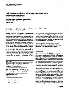
B. Network model Our network model consists of three tiers: Sensor nodes, On-demand cluster head and Mobile sink. By sending a Query packet to a WSN, the mobile sink queries a specific area or a point of interest for sensed data in the sensing field, where sensor nodes are densely and uniformly deployed. Each Query packet consists of the location information of the interested area. The sensor node closest to the center of the interested area elects itself as the cluster head, which we call an “ondemand cluster head”, and is responsible for gathering and aggregating the data in the interested area. The aggregated data (The Response packet) is then sent back to the mobile sink via multi-hop communication. As shown in Fig. 1, a vehicle is moving along a straight road, and queries a WSN deployed around the road. Such networks are appropriate for either environmental monitoring applications or the Intelligent Transportation Systems (ITS) [11], where the deployed WSNs enable vehicles to obtain the conditions of the surrounding environment, e.g., the status of parking slots along the street.
IV. QBDCS D ESIGN
Query
Response
V =γ·
d L R·DC
·
d r
=
dhop · R · DC , L dhop . r
0 1, the optimal query opportunity is when the mobile sink can just meet the r Response packet at (a, 0). when L Lq < 1, the optimal query opportunity is just when the mobile sink located at (a, 0). Er Vr 1 r Proof: let L Lq = k, we have Eq = k, Vq = k . To simplify the analysis, we assume tg ≈ 0, which will not affect the final result. The objective function can be written as Eq · min{d1 + k · d2 }, dhop
(13)
(0, 0)
(xoptimal, 0)
TABLE I S UMMARY OF THE QBDCS IN WSN S WITH MOBILE SINKS
(a, 0)
Vs
Mobile Sink
The best query time
x
Given Vs , R, r, Lq , Lr , DC , (a, b), dhop . Calculate The optimal query time (Xoptimal , 0) by Equation.(19) and the estimated meeting position.
d2 d1 Vr Vq
Data Source
y
r (a, b)
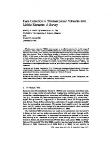
Fig. 3. Theoretical optimal query time based on meeting position aware r routing when L >1 L q
V
E
q can be regarded as a constant. Let Vqs = m, the where dhop constraint is p p (14) d1 + k · d2 = m · ( d21 − b2 + d22 − b2 ).
Applying Lagrange Multipliers method yields ( k · √ d21 2 − √ d22 2 = 0 d1 −b d2 −b p p d1 + k · d2 − m · ( d21 − b2 + d22 − b2 ) = 0.
(15)
Let d1 = b sec α and d2 = b sec β, α, β ∈ (0, π2 ). Equations.(15) can be written as ( k 1 sin α − sin β = 0 (16) sec α + k sec β − m tan α − m tan β = 0, which has boundary values when α = 0 or β = 0. Solving the Equations.(16), when k 6= 1, we have −2mk sin3 β + (m2 + k 2 + 1) sin2 β = 0.
(17)
Thus, sin β =
m2 +k2 +1 2mk
β ∈ (0, π2 ).
(18)
Obviously, Equation.(18) has no solution. Therefore, the objective function attains the optimal value when α = 0 or β = 0. When k > 1, it can be proven that the objective function has optimal value when β = 0, which is equivalent to the mobile sink and Response packet meeting at (a, 0). Based on the above analysis, when the Query packet is shorter than the Response packet in length, QBDCS finds the optimal query opportunity when the mobile sink is located at (xoptimal , 0), where p (a − xoptimal )2 + b2 b a − xoptimal + tg + − = 0. (19) Vq Vr Vs
Step 1: Querying at the right time. The mobile sink checks whether it is at the optimal query time. If yes, then it injects the Query packet towards the interested area. Step 2: Routing the Query packet. The Query is routed towards the interested area by adopting is the geographical location aware routing. Step 3: Data aggregation. Once the Query packet arrives at the targeted sensing area, the sensor node closest to the center of the interested sensing area elects itself as the cluster head and is responsible for gathering and aggregating the sensor data. Step 4: Routing the Response packet. The Response packet is then routed towards the mobile sink (estimated meeting position) until it arrives at the sensor node nearest to the estimated meeting position, which we call the “notifying node”. The “notifying node” checks whether the mobile sink has passed and is not in the sensor node’s radio range. If has not passed, the “notifying node” waits for the mobile sink to enter its radio range before delivering the Response packet. If has passed, the Response packet enters into the Chasing Mode until it catches up with the mobile sink. During this process, if exceeding the time limit Tdeadline , the Response packet should be discarded. Step 5: Response packet delivery. The Response packet is delivered to the mobile sink.
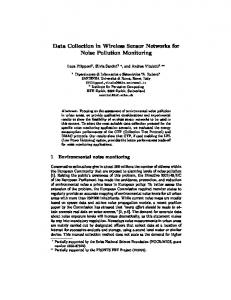
V. E VALUATION To evaluate the performance of the proposed QBDCS, we simulate an application scenario where sensor nodes are deployed in the sensing field densely and uniformly, using the simulation tool OMNeT++ [15]. We generate a rectangular grid with 50 × 20 cells. The side length of each cell is 30m. The mobile sink is moving on a straight road with a certain speed and may query an arbitrary interested area in the sensor deployed field. We define the vertical distance from the interested area to the road where the mobile sink is moving along as Query Distance (QD). For comparison, we also simulate the ”Naive” scheme, which the mobile sink sends the Query when locating at the nearest point from the interested area, as shown in Figure 4. Assume both of them adopt the MPAR protocol to forward the Response packet. The simulation starts from the mobile sink injecting a Query packet towards the interested area, and ends when mobile sink receives the Response packet. Injecting a Query when locating at the optimal query opportunity QBDCS
Injecting a Query when locating at the nearest point from the interested area
Naive Scheme
QD
(a, b)
E. Summary of QBDCS The Query-Based Data Collection Scheme is summarized in Table. I.
Fig. 4. Schematic of the routing paths in QBDCS and the “Naive” scheme under ideal condition
A. Performance metric
23.0 22.5
Vs=20 m/s 22.0
Vs=25 m/s 21.5
Delivery latency (s)
1) Delivery Latency: Delivery Latency is defined as the amount of time from injecting a Query packet by the mobile sink to the corresponding Response packet returning to the mobile sink. In QBDCS, the energy consumed in a WSN for transmitting a packet is proportional to its hop counts, which is also the determinant of the delivery latency. Minimizing the delivery latency and energy consumption in QBDCS are inherently unified. As a representative, the Delivery Latency is used as a performance metric in our simulation.
Vs=30 m/s 21.0 20.5 20.0 19.5 19.0 18.5 18.0 17.5 17.0 16.5 0.45
0.50
0.55
B. Simulation settings
0.65
0.70
0.75
0.80
0.85
0.90
0.95
Modification coefficient γ
The key communication parameters generally applies to IEEE 802.15.4. The velocity of mobile sinks varies from 20m/s to 30m/s. For simplicity, we assume the data aggregation time tg = 1 s. The data transmission rate R is taken 250kb/s, sensor transmission range r is taken 50m. CSM A/CA mechanism for collision management is adopted. Taking data-link layer CSM A/CA mechanism into consideration, about 40% overhead is introduced [9]. Thus, the data transmission rate under saturation condition is R0 = 150kb/s. Sensor nodes have a cycle time CT = 1s, DC = 1%. Assume the Query and Response packets length are Lq = 50 bytes and Lq = 127 bytes respectively. Therefore, the estimated delivery velocity Vq and Vr are r · R0 · DC ≈ γ · 187.5 m/s Lq
r · R0 · DC Vr = γ · ≈ γ · 73.8 m/s. Lr
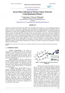
Fig. 5. The dependance of delivery latency on the modification coefficient γ in QBDCS
query opportunity. When the Response packet arrives at the “notifying node”, the mobile sink has already passed. The Response packet has to enter into the Chasing Mode, which increases both the delivery latency and energy consumption. That is the reason that the Response hop-count is more than the Query hop-count when γ is overestimated. 26 24 22
(20)
20 18
(21)
Let Dq and Dr denote the maximum delay of the Query and Response packets respectively. We have
Hop counts
Vq = γ ·
0.60
16 14 12 10
Query Hop-Count, Vs=30 m/s Response Hop-Count, Vs=30 m/s
8 6 4
Dq = Dr =
R0 Lq
1 ≈ 267 ms · CT · DC
R0 Lr
1 ≈ 677 ms. · CT · DC
(22)
2 0 0.50
0.55
0.60
0.65
0.70
0.75
0.80
0.85
0.90
Modification coefficient γ
(23)
C. Simulation results 1) Choosing the modification coefficient γ: The estimation of packet delivery velocity has direct effect on the performance of QBDCS. We simulate a mobile sink querying the area with Query Distance QD = 510 m. From Figure 5, it is shown that the optimal value for the modification coefficient γ is around 0.7, at which the QBDCS shows least delivery latency. Figure 6 depicts the change of the Query and Response hop-count in a query-based data collection cycle by increasing the value of γ when Vs = 30m/s. When γ is underestimated (smaller than 0.7), it results in sending Query packet earlier than the optimal query opportunity. Thus, the Query hopcount is more than the Response hop-count. In this case, the Response packet will arrive at the “notifying node” in advance and wait for the mobile sink, which increases the delivery latency. When γ is overestimated (larger than 0.7), it leads to sending Query packet later than the optimal
Fig. 6. The change of packet hop counts by increasing the value of γ in QBDCS
It is found that the optimal value of the modification coefficient γ depends on the sensor deployment strategy. As in our simulation, where sensor nodes are deployed in the sensing field densely and uniformly, forming a two dimensional grid, the optimal value of γ is about 0.7. 2) The impact of mobile sink velocity: We set the Query Distance to be 510m, and vary the mobile sink velocity from 20m/s to 30m/s. The modification coefficient γ is taken 0.7. Figure 7 depicts the effect of increasing mobile sink velocity on the delivery latency. As shown in Figure 7, QBDCS is insensitive to the variance of the mobile sink velocity. With the increase of the mobile sink velocity, the “Naive” scheme pays more cost. This is because that delivery latency of completing a query-based data collection cycle mainly depends on the hop counts of routing the Response packet. QBDCS can assure the least hop-count
during the Response Propagation phase.
sink velocity. In any case, QBDCS will not be worse than the “Naive” scheme. VI. C ONCLUSION
36
QBDCS Naive scheme
34
Delivery latency (s)
32 30 28 26 24 22 20 18 16 20
22
24
26
28
30
Mobile sink velocity (m/s)
Fig. 7.
Delivery Latency vs. mobile sink velocity
3) The impact of query distance: We vary this distance from 120m to 510m, to compare the differences when mobile sink velocity is set 25m/s and 30m/s respectively. The modification coefficient γ is taken 0.7. Obviously, the delivery latency and energy consumption depends on the Query Distance (QD). The longer Query Distance, the larger delivery delay and more energy consumption. As shown in Figure 8, with an increase of the Query Distance, the advantage of QBDCS becomes more significant. It is notable that the increasing speed of the delivery latency in QBDCS almost keeps consistent when Vs = 25m/s and Vs = 30m/s. For the “Naive” scheme, however, the increasing speed of the delivery latency increases as the mobile sink velocity increases. 40
QBDCS, Vs=30m/s Naive scheme, Vs=30m/s QBDCS, Vs=25m/s Naive scheme, Vs=25m/s
Delivery latency (s)
35
30
25
20
15
10
5 100
200
300
400
500
Query Distance (m)
Fig. 8.
Delivery Latency vs. Query Distance
D. Discussion In our simulation, we consider the general conditions when DC = 1%. Although QBDCS will be close to the “Naive” scheme when duty cycle DC is large enough or the mobile sink velocity is slow enough, which means that the estimated delivery velocity of a packet is much larger than the mobile
In this paper, we addressed the problem of query-based data collection in WSNs with mobile sinks. We estimated the packet delivery velocity and predicted the packet-sink meeting position. Then, we proposed an efficient Query-Based Data Collection Scheme (QBDCS), as the main contribution of this paper. QBDCS chooses the optimal query opportunity to send the Query packet and tailors the routing mechanism for partial node participation in a WSN. Through theoretical analysis and simulations, we illustrated that QBDCS achieved the performances of minimizing the energy consumption and delivery latency in a query-based data collection cycle. R EFERENCES [1] K. Romer and F. Mattern, “The design space of wireless sensor networks,” IEEE Wireless Communications, vol. 11, no. 6, pp. 54–61, Dec. 2004. [2] J. Ma, C. Chen, and J. P. Salomaa, “mwsn for large scale mobile sensing,” Journal of Signal Processing Systems, vol. 51, pp. 159–206, 2008. [3] S. Jain, R. C. Shah, W. Brunette, G. Borriello, and S. Roy, “Exploiting mobility for energy efficient data collection in wireless sensor networks,” Mobile Networks and Applications, vol. 11, no. 3, pp. 327–339, 2006. [4] L. Song and D. Hatzinakos, “Architecture of wireless sensor networks with mobile sinks: Sparsely deployed sensors,” IEEE Transactions on Vehicular Technology, vol. 56, no. 4, pp. 1826–1836, July 2007. [5] P. P. Jayaraman, A. Zaslavsky, and J. Delsing, “Sensor data collection using heterogeneous mobile devices,” Pervasive Services, IEEE International Conference on, pp. 161–164, 15-20 July 2007. [6] W. Heinzelman, A. Chandrakasan, and H. Balakrishnan, “Energyefficient communication protocol for wireless microsensor networks,” System Sciences, 2000. Proceedings of the 33rd Annual Hawaii International Conference on, pp. 10 pp. vol.2–, Jan. 2000. [7] L. Kulik, E. Tanin, and M. Umer, “Efficient data collection and selective queries in sensor networks,” pp. 25–44, 2008. [8] R. Teng, B. Zhang, and Y. Tan, “A study of localized on-demand data collection in sensor networks,” Networks, 2007. ICON 2007. 15th IEEE International Conference on, pp. 431–436, Nov. 2007. [9] D. Tacconi, I. Carreras, D. Miorandi, I. Chlamtac, F. Chiti, and R. Rantacci, “Supporting the sink mobility: a case study for wireless sensor networks,” IEEE International Conference on Communications, ICC ’07., 2007. [10] M. Battelli and S. Basagni, “Localization for wireless sensor networks: Protocols and perspectives,” Electrical and Computer Engineering, 2007. CCECE 2007. Canadian Conference on, pp. 1074–1077, April 2007. [11] M. Tubaishat, P. Zhuang, Q. Qi, and Y. Shang, “Wireless sensor networks in intelligent transportation systems,” Wireless Communications and Mobile Computing, pp. 1530–8669, 2008. [12] B. Karp and H. T. Kung, “Gpsr: Greedy perimeter stateless routing for wireless networks,” in In Proceedings of the Sixth Annual ACM/IEEE International Conference on Mobile Computing and Networking, 2000, pp. 243–254. [13] L. Shu, Y. Zhang, Z. Zhou, M. Hauswirth, Z. Yu, and G. Hynes, “Transmitting and gathering streaming data in wireless multimedia sensor networks within expected network lifetime,” Mob. Netw. Appl., vol. 13, no. 3-4, pp. 306–322, 2008. [14] J. A. T. Chipara, O. Zhimin He Guoliang Xing Qin Chen Xiaorui Wang Chenyang Lu Stankovic, “Real-time power-aware routing in sensor networks,” 14th IEEE International Workshop on Quality of Service, 2006. IWQoS 2006., pp. 83–92, June 2006. [15] “Omnet++ discrete event simulation system.” [Online]. Available: http://www.omnetpp.org