Jun 30, 2009 - queries and repeating the original query on the randomized tables. It turns out that ...... izing in different relations matters for that query. For most.
Query Significance in Databases via Randomizations Markus Ojala ∗
Gemma C. Garriga ∗
Aristides Gionis †
Heikki Mannila ∗
June 30, 2009
arXiv:0906.5485v1 [cs.DB] 30 Jun 2009
Abstract
GM
Many sorts of structured data are commonly stored in a multi-relational format of interrelated tables. Under this relational model, exploratory data analysis can be done by using relational queries. As an example, in the Internet Movie Database (IMDb) a query can be used to check whether the average rank of action movies is higher than the average rank of drama movies. We consider the problem of assessing whether the results returned by such a query are statistically significant or just a random artifact of the structure in the data. Our approach is based on randomizing the tables occurring in the queries and repeating the original query on the randomized tables. It turns out that there is no unique way of randomizing in multi-relational data. We propose several randomization techniques, study their properties, and show how to find out which queries or hypotheses about our data result in statistically significant information. We give results on real and generated data and show how the significance of some queries vary between different randomizations.
=
{(Romance, m1 ), (Romance, m2 ), (Drama, m3 ), (Drama, m4 ), (Drama, m5 ), (Drama, m6 ), (Drama, m7 ), (History, m6 ), (History, m7 )}
MD
=
{(m1 , C. Waitt), (m2 , C. Waitt), (m3 , C. Waitt), (m4 , C. Waitt), (m5 , C. Waitt), (m6 , T. George), (m7 , T. George)}
DA
=
{(C. Waitt, 30), (T. George, 60)}
Figure 1: A toy example of a multi-relational database consisting of three binary relations: movies classified by genre, GM; directors of movies, MD; and ages of directors, DA.
been extended as well to the data mining and database community. In a very first paper about association rules, Brin et al. [14] considered measuring the significance of rules via the chi-squared test, and from there many other papers followed—see e.g. [15] for a comprehensive survey. More recently, the approach of defining randomization tests to assess data mining results was introduced for binary data [8], and for real-valued data [12]. Abstracting a bit from the question of how significant patterns are in the data, we introduce here the statistical testing framework to databases and the exploratory task of querying the relations of the database. The question of understanding what we know and what we believe about our dataset becomes tricky when the data is highly structured and interrelated. Structured data is everywhere: examples are the Internet Movie Database (IMDb), or the DBLP computer science bibliography, and indeed, most of today’s information systems are actually relational databases. In IMDb, e.g., basic entities are directors, movies, genres, ranks or years; in addition, we have relations such as directors direct movies, movies are classified by a genre, movies are ranked with some quality criteria, and directors are born in a certain year. Each of these relations is represented in a separate table which relates to others through their common attribute values. A simple toy example is given in Figure 1. In multi-relational databases, users and applications access the data via queries. E.g., a query can be made to check the average age of directors of history movies, or the average age of directors of romance movies. In the toy exam-
1 Introduction The question of evaluating whether certain hypotheses made from observed data are significant or not, is one of the oldest problems in statistics. Statistical significance reduces an observed result (statistic) to a p-value that tells about the probability of observing the same result at random when a certain null hypothesis is true. If this p-value is sufficiently small, we can assume that the null hypothesis is false. The technical challenge of defining an exact p-value for a given hypothesis is typically resolved by studying the null distribution of the test analytically; for example, the well known chi-squared test is based on statistics that follow a chi-square distribution under the null hypothesis. Alternatively, when analytical solutions are not possible or hard to state exactly, the null distribution can be defined via permutation tests. These useful statistical concepts have been used for years in experimental fields such as medicine, biology, geology or physics, to name a few. Many of these considerations have ∗ HIIT, Department of Information and Computer Science, Helsinki University of Technology, Finland † Yahoo! Research, Barcelona, Spain
1
ple of Figure 1, the first query returns a value of 60, while the second query returns a value of 30. Usually, the answer returned by the query is assumed as a fact, thus implying some conventional wisdom—for this toy example we might be tempted to believe that directors of romance movies are younger than directors of history movies. But, should we really believe that this hypothesis is significant from the data? If we knew that all history movies are also classified as drama movies, would the value of 60 still have the same importance? Or, if we knew that the same director has participated in both romance and drama movies? We study whether the results returned by queries are significant or just a random artifact due to the structure in the data. Our statistical tool is randomizations and the approach is simple: randomize certain relations occurring in the queries and repeat the original query in the random samples. This provides an empirical p-value, and, as in basic statistics, we can reject or accept our hypothesis linked to the query. The goal behind this idea is to provide an understanding of how the structure of the data affects the significance of the information we derive from our queries. If certain structures or patterns remain after simple randomizations (e.g., the fact that history movies are also drama movies in the toy example), the answers of a query that rely on such patterns should be regarded as not significant. It turns out that there is no unique way of randomizing in multi-relational data, and indeed, it is difficult to give a fully satisfactory answer about which randomizations are more important than others. We study several randomization methods and show the combinatorial properties of the null distributions on multiple tables. Our contribution makes a first step towards understanding how the significance of a query is linked to the structure hidden in the data; randomizations are a sound statistical tool to make such a connection. We believe this is an important problem of interest to both the database and data mining communities. We present experimental results on synthetic data, and show the usability of the method for several queries in real datasets.
Romance Drama History
m1 1 0 0
m2 1 0 0
m3 0 1 0
m4 0 1 0
m5 0 1 0
m6 0 1 1
m7 0 1 1
C. Waitt T. George
30 1 0
60 0 1
(a) Genre × Movie
m1 m2 m3 m4 m5 m6 m7
C. Waitt
T. George
1 1 1 1 1 0 0
0 0 0 0 0 1 1
(c) Director × Age
(b) Movie × Director
Figure 2: The binary table representation of the toy database in Figure 1: (a) GM; (b) MD; and (c) DA. 1 0 111111 000000 0000000 1111111 000000 111111 0000000 1111111 000000 111111 0000000 1111111 000000 111111 0000000 1111111 000000 111111 0000000 1111111 1 0 000000 111111 0000000 1111111 000000 111111 0000000 1111111 000000 111111 0000000 1111111 000000 111111 0000000 1111111 11 Romance00 000000 111111 0000000 1111111 0000000 1111111 0000000 1111111 0000000 1111111 0000000 1111111 1 0 1 0 1 30 0 0000000 1111111 1111111 0000000 0000000 1111111 111111 000000 0000000 1111111 0000000 1111111 0000000 1111111 0000000 1111111 0000000 1111111 0000000 1111111 0000000 1111111 0000000 1111111 1 0 1111111 0000000 11 Drama00 0000000 1111111 0000000 1111111 0000000 1111111 0000000 1111111 0000000 1111111 0000000 1111111 0000000 1111111 0000000 1111111 1 0 0000000 1111111 0000000 1111111 0000000 1111111 1 0 1 60 0 0000000 1111111 1111111 0000000 0000000 1111111 00 0000000 1111111 History11 0000000 1111111 0000000 1111111 00 11 0000000 1111111 0 1 0000000 1111111 0000000 1111111 0000000 1111111 0 1 0000000 1111111 0000000 1111111 0000000 1111111 0000000 1111111 0000000 1111111 0000000 1111111 0000000 1111111 0000000 1111111 0000000 1111111 0000000 1111111 0000000 1111111 0 1 0000000 1111111 0000000 1111111 0000000 1111111 0 1 0000000 1111111
Figure 3: The bipartite graph representation of the movie database shown in Figure 2. The graph shows all the possible paths from the source nodes, Genre, to the destination nodes, Age.
join. Conceptually, a join between two relations A and B, denoted A⋊ ⋉B, combines all entries from A and B that share common attribute values to return a composition of the relations. For example, given (i, j) ∈ A, (j, k) ∈ B and (j, k ′ ) ∈ B, we have (i, j, k) ∈ A⋊ ⋉B and also (i, j, k ′ ) ∈ A⋊ ⋉B. The join operator is associative over a set of relations and its result explicitly represents all existing paths between the occurring relations. For example, the natural join of the three tables in Figure 2 returns a tuple for each path there is between Genre and Age. For an ordered subset of binary relations from the database S ⊆ {A1 , . . . , An }, we use ⋊ ⋉S to denote the final join between all elements in S. The order in S is to ensure a join of consistent relations; we assume that S in ⋊ ⋉S is always implicitly ordered. A query q is applied to the join of a subset of the relations in the database S ⊆ {A1 , . . . , An }. The result of a query is denoted by q(⋊ ⋉S). We say that S is the set of relations occurring in the query. A query can be described with the operators of projection and selection [13], applied to a join ⋊ ⋉S. Projection is a unary operator πX (⋊ ⋉S) that restricts tuples of ⋊ ⋉S to attributes in X. Selection is a unary operator
2 Problem statement Let A be a binary relation A ⊆ I × J between sets I and J. In the market basket application, for example, I could be a set of customers and J a set of products. A binary relation A ⊆ I × J identifies which customers from I buy which products from J. Notice that every binary relation can be seen as a binary matrix describing the occurrences between the row set I and column set J, see Figure 2 for examples. Let {A1 , . . . , An } be a set of n binary relations representing some structured data. This relational model is very general. It applies, for example, to a movie database system, as shown in Figure 2. The representation of the same example as a sequence of bipartite graphs is depicted in Figure 3. The basic operator to combine relations is the natural 2
σϕ (⋊ ⋉S) where ϕ is a propositional formula. The operator selects all tuples in the relation ⋊ ⋉S for which ϕ holds. Consider the movie database in Figure 2. A possible query is: select drama movies and project movie and age of its director. We can write this query as follows,
Romance Drama History
30 1 1 0
60 0 1 1
Romance Drama History
(a) GM · MD · DA
30 2 3 0
60 0 2 2
(b) GM ∗ MD ∗ DA
Figure 4: (a) Binary relation Genre × Age obtained via boolean product between GM · MD · DA of Figure 2; (b) Contingency table of paths between Genre and Age obtained via matrix product of GM ∗ MD ∗ DA.
q1 = πMovie,Age (σGenre = Drama (GM⋊ ⋉MD⋊ ⋉DA)) The result of query q1 is a set of pairs: {(m3 , 30), (m4 , 30), (m5 , 30), (m6 , 60), (m7 , 60)}. Another very similar query is: select drama movies and project age only. That is, q2 = πAge (σGenre = Drama (GM⋊ ⋉MD⋊ ⋉DA))
certain drug via permutation tests between the control and case group [9]. For short, let R =⋊ ⋉S for some S ⊆ {A1 , . . . , An }. To assess the significance of f (q(R)), we generate randomized versions of R and run the same query over the samples. Let ˆ = {R ˆ 1, . . . , R ˆ k } be a set of randomizations of R. We R will specify in Section 4.1 how to generate such randomized versions of R. Then the one-tailed empirical p-value of f (q(R)) with the hypothesis of f (q(R)) being small is,
Query q2 returns:{30, 60}. Although queries q1 and q2 are very similar, the projection made by q2 on only Age, has eliminated repeated values. The results of query q1 tell us how many paths there are between directors of Drama and Age, while in query q2 we only know if a path exists or not. Our goal is to assess whether the results returned by a query provide significant information about our hypothesis on the data. For simplicity, a statistic f is required to map the results of a query to a single real value. We assume this function f is provided by the user together with the query; they define the hypothesis on the data the user wants to test. Examples of this statistic are the average of the returned results, or the number of tuples in the answer, but indeed f can be any general function returning a real value. For example, the average value of Age in query q1 is 42.5 (i.e., the average age of directors of Drama weighted by the number of directed movies). Then, we may want to know whether that average age is interesting or not. Another twotailed hypothesis is whether that average is significantly different from the average age of directors of romance movies. Formally, our problem reads as follows.
ˆ∈R ˆ : f (q(R)) ˆ ≤ f (q(R))}| + 1 |{R . k+1
(1)
This definition represents the fraction of randomized samples having a smaller value of the statistic f . If the p-value is small, e.g., below a threshold value α = 0.05, we can say that the value of f (q(R)) is significant in the original data. The one-tailed p-value with the hypothesis of f being large and the two-tailed p-value are defined similarly.
3.2 Where to randomize? ˆ that is, the differThe challenge is how to generate the set R, ent randomized versions of R =⋊ ⋉S, to compute the empirical p-value. Consider the toy example in Figure 2. Suppose we want to evaluate whether the average age of the directors of drama movies, as in query q2 of Section 2, is young. A first naive approach is to consider randomizing directly the binary matrix obtained from the boolean product of all relations from Genre to Age. The boolean product tells us whether there is a path from the set of nodes of Genre to the set of nodes of Age, as required by query q2 . A traditional permutation test1 on this new matrix shown in Figure 4(a) can produce only two possible random samples: either the original matrix, or a matrix where the age values between Romance and History are swapped. For the particular case of romance movies with the hypothesis of having small age, we would obtain a p-value close to 0.5 (i.e. 50% of the randomized samples would have the same value as the original). Thus the result is not significant. In-
Problem 1 Given a set of binary relations {A1 , . . . , An } of structured data and a query q on some occurring S ⊆ {A1 , . . . , An }, is the value of f (q(⋊ ⋉S)) for a statistic f , significant (in some sense to be made more specific later)?
3 Overview of the method In this section we present an overview of the approach and describe the intuition behind it. We show how our method can be used to test the significance of queries and to uncover the structurally important relations in the data.
3.1 Significance testing via randomizations We approach the problem of testing the statistical significance of the query via randomizations. Randomizations have been widely used as a method to generate samples from null distributions. For example, in medical studies it is customary to measure the effect of a
1 A traditional permutation test would swap any values in the matrix, while keeping the row and column sums fixed. In binary data this is called swap randomization.
3
3.3 Example
Algorithm 1 Query significance in multi-relational data Input: A set of binary relations S ⊆ {A1 , . . . , An }, a query q(⋊ ⋉S) and a hypothesis over the statistic f (q(⋊ ⋉S)) Output: A set of p-values 1: for each binary relation A ∈ S do 2: Obtain k random samples of A, Aˆ = {Aˆ1 , . . . , Aˆk } ˆ A = {⋊ 3: Let R ⋉T ∪ Aˆ | Aˆ ∈ Aˆ and T = S\A} ˆA 4: Compute the p-value using the random samples R 5: end for
We study now the toy example in Figure 2. Consider a query defined such as q1 from Section 2, yet on the three different Genres. The first hypothesis that romance movies are directed by young directors obtains a p-value of 0.131 when randomizing on GM, a p-value of 0.494 on MD, and a p-value of 0.495 on MA. The hypothesis is not significant under any randomization, but we observe that randomizing on GM obtains the smallest p-value for this query. The hypothesis that history movies are directed by old directors obtains p-values 0.269, 0.045, 0.495 when randomizing on GM, MD, DA, respectively. Thus the hypothesis is significant considering the structure in relation MD: all non-history movies are directed by the same person. Finally, the hypothesis that drama movies are directed by young directors is not significant in any of the randomizations, always with a p-value close to 1 when randomizing on GM or MD, and p-value of 0.495 when randomizing on DA. In summary: the age value of 30 associated to romance movies is close to being significant when randomizing on GM because Romance is a non-intersecting genre with Drama and History; the age value of 60 associated to history movies is significant when randomizing on MD because, when focusing on the directors, the history movies are nonintersecting with the romance and drama movies—all romance and drama movies are directed by the same person; also, the relation DA always swaps with equal probability, because of its one-to-one structure. In the next section we will understand better the reason of these explanations.
deed, under such randomization none of the three genres would test significantly small, nor large, nor different. Alternatively, we could apply a permutation test on the contingency table of paths [4], shown in Figure 4(b). This table gives the number of paths between the Genre and Age, as required by q1 . The hypothesis related to our queries under those permutation tests would never be significant. The problem of these naive approaches is that they ignore the structure of the relations occurring in the query. In our toy example there are three binary relations participating in the query: GM, MD and DA. Indeed these relationships convey some structure on the data: the relation MD shows that all history movies are also drama movies; the relation MD shows that all movies from Drama and Romance have been directed by the same person. How do these structures affect the significance of the results in a query? In queries involving multiple binary relations, there is no unique way to randomize. To assess the structural effect that each relation from S has over the query q(⋊ ⋉S), we should randomize only the corresponding relation. That is, the different randomizations of ⋊ ⋉S are obtained by randomizing a single relation A ∈ S while keeping the rest fixed. More formally, the random samples of ⋊ ⋉S, when only A ∈ S is randomized, are defined as follows:
4 Randomizations in multi-relational model This section describes how to obtain random samples for a single relation A (line 2 in Algorithm 1), and presents the combinatorial properties of combining such samples with the other relations in the query (line 3 in Algorithm 1).
ˆ A = {⋊ R ⋉T ∪ Aˆ | Aˆ ∈ Aˆ and T = S\A}, where Aˆ = {Aˆ1 , . . . , Aˆk } is the set of randomized versions of the original A ∈ S. In Section 4.1 we describe the different randomization techniques to obtain such samples. Fiˆ A will be used to comnally, these randomized samples R pute the corresponding p-value, as described in Equation 1. Observe that for a given query involving relations in S, we can obtain one p-value for each A ∈ S we randomize (while keeping S\A fixed). Each p-value is interesting as it measures the structural effect that the participant relation A has on the significance of the result of the query. The sketch of the method is described in Algorithm 1. The basis of our proposal can be found in traditional statistics under the name of restricted randomizations (see e.g. [9], typically to test whether a treatment variable has effect on a response variable).
4.1 Types of randomization Given a binary relation A we use three different types of randomization to obtain random samples from A. The running times and space consumptions of the methods are linear in the size of the relation A. (1) Swap randomization of A, as used in [5, 8], produces random samples of A that preserve the row and column sums. The algorithm starts from A and performs local swaps interchanging a pair of 1’s with a pair of 0’s preserving the row and column sums. Technically, a local swap consists of selecting entries (i, j), (k, l) ∈ A 4
4.2 Properties
such that (i, l), (k, j) ∈ / A, and swapping the elements so that (i, j), (k, l) ∈ / A and (i, l), (k, j) ∈ A. On the bipartite graph representation of the relation A, a local swap represents a flip between two independent edges. i
j . . .
k
. . .
i
l
j . . .
⇐⇒
Next we study the properties of combining the obtained random samples with the other relations in the query. For simplicity, we study the case of queries with only two occurring relations q(A⋊ ⋉B) and use boolean product as a simplification of the natural join. For notational convenience, we overload the boolean product for the sets of binary matrices, e.g., sw(A) · sw(B) represents the boolean product of each pair of elements A ∈ sw(A) and B ∈ sw(B). The following inclusions with swap randomization follow immediately after the definitions. All other inclusions do not hold. The inclusions can also be proper in all cases.
k
. . . l
A sequence of swaps is performed until the data mixes sufficiently enough in a Markov chain approach [1, 2], and therefore, a random sample of A is obtained. We use ten times the number of ones in the matrix as the number of swaps, which suffices for the convergence of the chain [8]. We denote the set of all random samples reached via swap randomization of A as sw(A).
Proposition 2 Let A, B be binary matrices. Then: • A · B ⊆ sw(A) · B ⊆ sw(A) · sw(B); • A · B ⊆ A · sw(B) ⊆ sw(A) · sw(B);
(2) Row permutation of A permutes the order of the rows of A. We denote the set of all random samples reached via row permutation of A as rp(A).
• A · B ⊆ sw(A · B). Proposition 2 tells us that the set of samples that can be obtained by randomizing two relations is larger than by randomizing only one relation. As discussed in Section 3.2, we prefer to randomize a single table at a time in order to control much better the structural effect the randomized relation has on the query. Additionally, we know that the set of randomized samples sw(A) · B is different from the set A · sw(B), thus it makes sense to do them both separately. Next we present several properties relating swap randomization to row and column permutations.
(3) Column permutation of A permutes the order of the columns of A. We denote the set of all random samples reached via column permutation of A as cp(A). Note, particularly, that sw(A), rp(A) and cp(A) refer to sets of matrices. The relationship between swap randomizations and permutations can be stated as follows. Proposition 1 Let A be a binary matrix. Then: • rp(A) = sw(I) · A, where I is an identity matrix;
Proposition 3 Let A, B be binary relations. If B is a oneto-one relation, then A · sw(B) = cp(A). If A is a one-toone relation, then sw(A) · B = rp(B).
• cp(A) = A · sw(I), where I is an identity matrix; • if A has one 1 in each row, then sw(A) = rp(A); if A has one 1 in each column, then sw(A) = cp(A).
Proposition 3 follows immediately from Proposition 1. In real world datasets, it is quite common to have one-to-one relations. For example, the ages of the directors in the example in Figure 2 are one-to-one. Thus swap randomization of the relation DA produces the same set of samples as the column permutation of MD.
Note that sw(I), for identity matrix I, can produce any swap permutation matrix with uniform distribution. Thus, we have that the boolean product sw(I) · A produces all permutations for the rows of A and similarly, A · sw(I) produces all permutations of the columns of A. Intuitively, these row (or column) permutations can be seen as a random re-assignment of the row (or column) names in A. While the swap randomization has been used in [8] to assess the data mining results on a single binary relation, the new randomizations, corresponding to row and column permutations, do not make sense in such a context. The row or column permutation of a matrix does not change any of the frequent pattern solutions in the new randomized matrix. These permutations only make sense in a multi-relational data model, where the permuted matrices are combined with other relations. Both row and column permutation of a single relation change the global paths from the source nodes to destination nodes in the query graph, and thus, the evaluation of the query can change on the randomized data.
Proposition 4 Let A, B binary relations. Then: • cp(A · B) = A · cp(B) • rp(A · B) = rp(A) · B • cp(A) · B = A · rp(B) = cp(A) · rp(B) This means that column and row permutations do not make sense in more than one relation, e.g., A · cp(B · C · D) · E = A · B · C · cp(D) · E. The last property of Proposition 4 states that only one permutation, either column permutation on A or row permutation on B, is indeed necessary. Finally, we give an implication of Proposition 1 that reduces the number of different randomizations considerably.
5
Theorem 1 Let A, B be binary relations. Then: A · sw(I) · B = cp(A) · B = A · rp(B), where I is an identity matrix.
samples in the null distribution have the history movies connected to the age of 30. The hypothesis of history movies being directed by a not-so-young person is then significant.
Hence, we prefer to use the notation with the identity matrix I to refer to the row and column permutations. The operation A · sw(I) · B randomizes the boolean product, whereas the operations sw(A) · B and A · sw(B) randomize the original data. From this perspective, A · sw(I) · B tells about the significance of the combination operation, while sw(A) · B tells whether the structure in A is significant. To sum up, we have the following result:
5 Studying path distributions For a query q(A⋊ ⋉. . .⋊ ⋉B) where A ⊆ I ×L and B ⊆ J ×K, let P = A ∗ . . . ∗ B be the matrix product of all relations participating in q. This corresponds to the contingency table of paths from origin I to destination nodes K. An example is shown in Figure 4(b) for the toy data of Figure 2. For all types of queries, the significance of the result is closely related to the path distributions between nodes I and K. For example, suppose we want to test whether the average age of history-movie directors is large. In the original data of Figure 3 there are two paths from History to the age of 60 and no path to the age of 30. It is sensible to assume that if we had random samples where paths are mainly swapped the other way round, the hypothesis would be significant. Naturally, a simple way to visualize whether there exists an interesting finding in the data is to compare the path distribution of P with the expected path distribution on the given random samples. The larger the change, the more significant the result would tend to be. The following three matrices show the expectation of the paths when swap randomizing relation GM, MD or DA, respectively, for the example in Figure 2.
Corollary 1 For a query q(A⋊ ⋉B), there exist three different randomizations: (i) sw(A) while keeping B fixed; (ii) sw(B) while keeping A fixed; (iii) sw(I) where I is an identity relation between the columns of A and the rows of B. Notice that if A or B are one-to-one relations, then randomization (iii) will be the same as (i) or (ii) respectively. Each randomization provides a set of samples from where we can compute a p-value for our query (hypothesis on the data). Every p-value is interesting as it shows how the structure of the randomized relation affects the significance.
4.3 Example revisited The p-values reported in Section 3.3 for the toy example in Figure 2, correspond to swap randomization of the binary tables GM, or MD, or DA, respectively. Indeed because MD has one single 1 in each row, we have that GM · sw(I) · MD · DA is equal to GM · sw(MD) · DA. Similarly, because DA is a one-to-one relation, we have GM · MD · sw(I) · DA equals GM · MD · sw(DA). Thus, for this example, only swap randomization in the three tables is necessary. Interestingly, we can understand better now the p-values reported in Section 3.3. On the relation GM, drama movies and history movies have no independent edges to swap between them. Therefore, the pattern of History implying Drama tends to remain in random samples. As a result, the p-value of the hypothesis related to history or drama movies is not significant. On the other hand, the p-value related to romance movies becomes close to being significant because, for this genre, the null distribution diverges more from the original. The fact that there are only two romance movies raises this p-value slightly above the 0.05 threshold. Similar explanation goes when randomizing MD. When looking at MD, local swaps can interchange at most two edges between movies of the young director C. Waitt and movies of the not-so-young director T. George. Actually, in all random samples coming from MD we observe that C. Waitt has always at least three movies from either drama or romance. As a result, neither drama nor romance can be significant—in the null distribution they are always closely linked to a young director as in the original data. Yet, history movies directed by T. George have more local swaps that would create a diverging null distribution—most of the
E[sw(GM) ∗ MD ∗ DA]
0 0.849 @ 3.269 0.882
1
1.151 1.731 A 1.118
E[GM ∗ sw(MD) ∗ DA]
0
1.413 @ 3.587 1.455
1
0.587 1.413 A 0.545
E[GM ∗ MD ∗ sw(DA)]
0 0.984 @2.492 1.016
1 1.016 2.508A 0.984
The genre that swaps most of its paths under randomizations with GM is Romance. History swaps the paths from the age of 60 to the age of 30 when randomizing on MD. Randomization on DA distributes paths fifty-fifty for each genre. The p-values obtained there were always close to 0.5.
6 Empirical results In this section we present empirical results on synthetic and real datasets. Our real dataset is MovieLens, which is very similar to IMDb. In all cases, we calculate the empirical pvalues over 999 randomized samples and use the threshold of α = 0.05 to determine the query significance. The randomization methods are fast in practice. In our experiments, producing one randomized sample took approximately the same time as evaluating the query. With the tested datasets, the times for producing one sample were at most few seconds with Java implementations integrated with MATLAB on a 2.2GHz Opteron. The time and space consumption of the methods scale linearly in the size of the relation. In large-scale applications, fewer number of ran6
domized samples can be used to calculate the empirical pvalues. For example, 30 samples is usually sufficient in a preliminary significance analysis. This corresponds to approximately 30 times increase in the evaluation time.
M
M
F
F G1
G2
G3
G4
G5
G6
G1
(a) SU*UM*MG
6.1 Synthetic dataset
M
To motivate our approach and understand better why randomizations are consistent with the inferences about our hypothesis, we generate a synthetic dataset to simulate relations of users, movies and genres. We will be interested in testing the following hypothesis.
G2
G3
G4
G5
G6
(b) rSU*UM*MG M
F
F G1
G2
G3
G4
G5
G6
G1
(c) SU*rUM*MG
G2
G3
G4
G5
G6
(d) SU*UM*rMG
Figure 5: Proportion of paths going from a gender (M=male, F=female) to a genre (G1–G6) in the different combined tables. Lighter color represents less paths, while darker more paths; to be more exact: white corresponds to the lowest value of 4.5% and black to the highest value of 30%.
Hyp 1 Men watch different types of movies than women. The relations occurring in the query are: Gender×User (SU), User×Movie (UM) and Movie×Genre (MG). For studying the behavior of randomizations, we generate the tables SU, UM and MG to make our hypothesis clearly be significant. We let SU contain 30 men and 20 women, thus SU is a 2 × 50 binary table where the first 30 values in the first row and the last 20 values in the second row are 1s. We generate UM to be a 50 × 100 binary table where men watch any of the first 60 movies with probability of 0.40 and any of the last 40 movies with probability of 0.05. To create a strong pattern, we let the probabilities of a female watching movies be the other way round. Finally, we generate MG as a 100 × 6 binary table where the first three genres will be considered to be manly and the last three genres will be considered to be womanly. For each movie in the relation, we select two genres as follows: for the first 60 movies we select a genre from the manly genres with a probability of 0.9 and from the womanly genres with a probability of 0.1. For the last 40 movies the probabilities are the other way round. So, each movie has at most two genres, because if we happen to select the same genre for a movie twice, then we say that the movie has only one genre. Next we create the anti-tables from those above, called rSU, rUM and rMG. These anti-tables will not contain any structure at all, they are random. We let rSU be a 2 × 50 binary table with 30 men and 20 women where the order of the users is random. We generate rUM to be a 50 × 100 table with each element being 1 with a probability of (0.40+ 0.05)/2. And we let rMG be formed similarly to MG but with the two genres for each movie assigned uniformly with replacement. The goal of this experiment is to study how the p-values of Hyp 1 change when combining the original significant tables SU, UM and MG to one of these non-significant tables. Figure 5 shows the contingency table of paths from those combinations. We notice that using the original tables SU, UM and MG (Figure 5(a)) produces clearly a significant difference between the types of movies that males and females watch. By replacing one of the original tables with a random version, the pattern seems to disappear. Still, we cannot clearly see from the path distributions which of the
p-values
Input relations A
B
C
SU UM MG rSU UM MG SU rUM MG SU UM rMG
sw(IAB )
sw(B)
sw(IBC )
sw(C)
0.001 0.517 0.282 0.001
0.001 0.030 0.279 0.001
0.001 0.013 0.155 0.704
0.001 0.003 0.124 0.727
Table 1: Significance tests for the Hyp 1 with the combined input relations A⋊ ⋉B⋊ ⋉C. The first three columns contain the relations considered as input, labeled A, B and C. Columns 4th to 7th are empirical p-values for the hypothesis when only one relation is randomized: sw(IAB ) randomizes the identity matrix between relations A and B, which is equivalent to randomizing the relation A, sw(A); sw(B) randomizes only on relation B; sw(IBC ) randomizes the identity matrix between relations B and C; sw(C) randomizes only relation C. Bold p-values correspond to randomizations which touch the anti-tables. underlying tables mainly breaks the original structure. We would like to check with our tests whether randomizing in the proper tables will tell us where the pattern is broken. For the test, we use the following statistic. Statistic 1 L1 distance between the distribution of genres of the movies that men and women have watched. This statistic is the sum of the absolute differences between the proportion of paths of men and women, as shown in Figure 5 for each of the combinations. The original value of the statistic with the tables SU, UM and MG is 1.23, implying a clear difference between males and females. When one of the tables SU, UM and MG is replaced with a corresponding anti-table, the value of the L1 statistic is around 0.1. In Table 1 we show the results of the several significance tests for the hypothesis Hyp 1 on the several combined tables. There is a clear connection between the structure of the relations A, B and C occurring in the query and the p7
Relation
Description
Rows
Cols
# of 1’s/row
UM MG UO US UA
User×Movie Movie×Genre User×Occupation User×Gender User×Age
943 1680 943 943 943
1680 18 21 2 943
106 1.7 1 1 1
SU⋊ ⋉UM⋊ ⋉MG sw(SU)⋊ ⋉UM⋊ ⋉MG SU⋊ ⋉sw(I)⋊ ⋉UM⋊ ⋉MG SU⋊ ⋉sw(UM)⋊ ⋉MG SU⋊ ⋉UM⋊ ⋉sw(I)⋊ ⋉MG SU⋊ ⋉UM⋊ ⋉sw(MG)
Table 2: Summary of tables in MovieLens dataset. The table UA is an identity map between users and their ages. We denote a transpose by reversing the relation name.
Mean
(Std)
p-value
0.16 0.03 0.03 0.01 0.03 0.02
(0.01) (0.01) (0.00) (0.01) (0.00)
0.001 0.001 0.001 0.001 0.001
Table 3: Significance evaluation of Hyp 2. Mean and std are the average and standard deviation of Statistic 2 in the original input data (first row) and several randomizations.
values obtained by randomizing in different relations. As expected, the empirical p-value of Hyp 1 with tables SU, UM and MG is significant with randomizations in all tables. On the other hand, when one of the clearly-structured tables SU, UM or MG is replaced by the anti-tables rSU, rUM or rMG respectively, we obtain large empirical p-values for those randomizations that touch the anti-tables (see the bold values of Table 1). This illustrates how randomizations can tell about the structural effects in the significance of a query.
Genre, corresponding to relations SU, UM and MG. There are five different types of randomizations of the query which each produce a unique p-value. The results in Table 3 show that Hyp 2 is significant wrt all different randomizations. Indeed, the results on Hyp 2 seem to indicate that men watch movies with different genres than women. All randomizations are consistent. We will next analyze which genres separate men and women. We repeat the following hypothesis (with associated query) for each genre G.
6.2 MovieLens dataset
Hyp 3 Men watch genre G more (or less) than women.
The MovieLens data is collected through the MovieLens web site (movielens.umn.edu). The downloadable data is already cleaned up, i.e., users who had less than 20 ratings or did not have complete demographic information were removed from the data set. In all, the data consists of 100,000 ratings (valued from 1 to 5) from 943 users on 1,682 movies. Each user has rated at least 20 movies and the demographic information for the users correspond to attributes of age, gender, occupation and zip code. For each movie we have title, release year and a list of genres. Furthermore, we interpret that if a user has rated a movie, it means that he or she has watched it. This corresponds to the binary table named UM. We do not use the information of ratings in any other way. In Table 2 we summarize the binary relations in the MovieLens dataset. The table UA is just an identity matrix which maps the users to their ages, thus two different columns of the table UA may correspond to the same age. Handling numerical values in this way guarantees that two users having the same age are not combined into a single user after a join and a projection. Next, we go through a few queries on the dataset and analyze their significances.
Statistic 3 The difference between the %-proportions of the movies from genre G among all the movies men and women have watched. Notice this statistic is similar to Statistic 2 but now we only look at the difference for the specific genre G. The empirical p-values of the significance testings of Hyp 3 are given in Table 4. Again we find out that randomizing in different relations produces fairly similar results in general. We can observe that men watch significantly more, for example, action and sci-fi movies than women, whereas women watch significantly more romance and drama movies than men. Interestingly, we can say the popularity of mystery and documentary movies do not depend on the gender. Actually the genres which have the smallest amount of movies are the least significant ones. The genres with fewest number of movies are fantasy (with 22 movies), film-noir (24), western (27), animation (41) and documentary (50). Next we study users by their occupation. Hyp 4 The users with occupation O watch different types of movies than other users. Statistic 4 L1 distance between the distributions of genres of the movies watched by users with occupation O and users with other occupations.
Hyp 2 Men watch different types of movies than women. Statistic 2 L1 distance between the distribution of genres of the movies that men and women have watched.
The results of the significance testings are given in Table 5. When evaluating the associated query, we find that randomizing in different relations matters for that query. For most of the occupations, Hyp 4 is not significant when randomizing on sw(OU)⋊ ⋉UM⋊ ⋉MG nor OU⋊ ⋉sw(I)⋊ ⋉UM⋊ ⋉MG.
In Table 3 we give the empirical p-values for Hyp 2. Each row shows the relation being randomized for obtaining the corresponding p-value. The query associated to the hypothesis traverses the relations Gender × User × Movie × 8
G Action Sci-fi Thriller Adventure Crime War Horror Western Film-noir Mystery Document. Fantasy Animation Musical Children’s Comedy Drama Romance
Orig. sw(SU) sw(I1 ) sw(UM) sw(I2 ) sw(MG) 2.5 1.5 1.1 0.8 0.6 0.5 0.4 0.2 0.1 0.0 0.0 -0.1 -0.2 -0.5 -1.0 -1.3 -2.3 -2.3
0.001 0.001 0.001 0.001 0.002 0.002 0.019 0.001 0.012 0.392 0.404 0.064 0.032 0.001 0.001 0.001 0.001 0.001
0.001 0.001 0.001 0.001 0.001 0.001 0.018 0.001 0.009 0.401 0.392 0.070 0.033 0.001 0.001 0.001 0.001 0.001
0.001 0.001 0.001 0.001 0.001 0.001 0.001 0.001 0.001 0.395 0.391 0.051 0.001 0.001 0.001 0.001 0.001 0.001
0.001 0.001 0.001 0.001 0.001 0.004 0.011 0.005 0.054 0.424 0.468 0.243 0.027 0.001 0.001 0.001 0.001 0.001
sw(I2 )
sw(OU)
Orig. Mean (Std) p-val. Mean (Std) p-val.
0.001 0.001 0.001 0.001 0.002 0.002 0.020 0.003 0.058 0.469 0.489 0.201 0.018 0.001 0.001 0.001 0.001 0.001
None Librarian Retired Homemaker Doctor Entert. Educator Lawyer Salesman Healthcare Student Scientist Artist Technician Programmer Engineer Marketing Writer Executive Administr. Other
Table 4: Empirical p-values for Hyp 3. The values for the associated Statistic 3 in the original relations are given in the second column. The different randomizations methods (columns 3rd to 7th) correspond to randomizing in one relation at a time from SU⋊ ⋉I1 ⋊ ⋉UM⋊ ⋉I2 ⋊ ⋉MG. Genres are sorted by the value of the statistic. Significance tests say: genres over the first dashed line are more watched by men (p-values always under 0.05); genres under the second dotted line are more watched by women (p-values always under 0.05). We cannot say anything about genres in between the two dotted lines.
0.23 0.18 0.18 0.17 0.15 0.14 0.13 0.13 0.12 0.12 0.11 0.11 0.10 0.10 0.08 0.08 0.08 0.08 0.07 0.05 0.04
0.13 0.05 0.10 0.14 0.14 0.09 0.04 0.11 0.11 0.09 0.03 0.07 0.07 0.07 0.05 0.05 0.07 0.06 0.07 0.04 0.04
(0.05) (0.02) (0.04) (0.05) (0.05) (0.03) (0.01) (0.04) (0.04) (0.03) (0.01) (0.02) (0.03) (0.03) (0.02) (0.02) (0.03) (0.02) (0.02) (0.02) (0.01)
0.038 0.001 0.040 0.269 0.373 0.073 0.001 0.237 0.330 0.211 0.001 0.052 0.130 0.183 0.025 0.034 0.340 0.122 0.337 0.367 0.483
0.07 0.04 0.05 0.15 0.08 0.04 0.03 0.05 0.06 0.04 0.03 0.05 0.04 0.03 0.03 0.03 0.05 0.03 0.04 0.02 0.02
(0.01) (0.01) (0.01) (0.03) (0.02) (0.01) (0.01) (0.01) (0.01) (0.01) (0.01) (0.01) (0.01) (0.01) (0.01) (0.01) (0.01) (0.01) (0.01) (0.01) (0.00)
0.001 0.001 0.001 0.226 0.001 0.001 0.001 0.001 0.001 0.001 0.001 0.001 0.001 0.001 0.001 0.001 0.006 0.001 0.001 0.001 0.002
Table 5: Empirical p-values for Hyp 4. The original values of Statistic 4, with mean and std over 999 randomized samples are given. The results on randomizations OU⋊ ⋉ sw(I1 )⋊ ⋉UM⋊ ⋉MG were similar to sw(OU)⋊ ⋉UM⋊ ⋉MG, whereas the results on OU⋊ ⋉sw(UM)⋊ ⋉MG and OU⋊ ⋉UM⋊ ⋉ sw(MG) were similar to OU⋊ ⋉UM⋊ ⋉sw(I2 )⋊ ⋉MG. Bold pvalues are significant with sw(OU) and nonsignificant with sw(I2 ).
For the other randomizations we have that all occupations, except for homemakers, exhibit significance of the hypothesis. We observe that the largest occupation groups of librarians (51), educators (95) and students (196) have the most significant empirical p-values for the query, with all type of randomizations. We could infer that those type of users watch different genres than other users.
crime and fantasy are not significant, whereas the results on other genres are significant. Thus the inner structure of the User×Movie and Movie×Genre relations explain the results of our query. The average ages of the users of the genres with a star in Table 6 were significant with all types of randomizations.
Hyp 5 Average age of the users who have watched movies of a given genre is significant.
7 Related work
Statistic 5 Weighted average age of the users who have watched movies of the given genre.
Obviously, there is a large amount of statistical literature about hypothesis testing [3, 9]. For the particular case of data mining, many papers work on the significance of association rules and other patterns [14, 15]. In the recent years, the framework of randomizations has been introduced to the data mining community to test significance of patterns: the papers [5, 8] deal with randomizations on binary data, and the work in [12] studies randomizations on real-valued data. For another type of approach to measuring p-values for patterns, see [16]. A related work that studies permutations on networks and how this affects significance of patterns is [11]. Sub-sampling methods such as bootstrapping [7]
The results of assessing Hyp 5 are given in Table 6. The empirical p-values of the queries depend largely on the type of randomization used. By randomizing the ages of the users, that is, sw(AU)⋊ ⋉UM⋊ ⋉MG, the movies whose average age of watchers has originally been around 34 years are not significant. This makes sense when it is compared to the average of all users which is 34.1 years. Notice that in the query the average is weighted by the number of movies watched by the user. Thus randomizing the table AU tests the connection between the ages and the users. Other randomization points tell us that the results on western, romance, 9
important first step towards understanding how the structure hidden in the data makes some hypotheses more significant than others, but still, a lot of interesting future work needs to be done: study of the combinatorial properties and its connection to the significance of queries and patterns.
Orig. sw(AU) sw(UM) sw(I2 ) sw(MG) Film-noir* Documentary Mystery War Drama Western Romance* Musical Crime Comedy* Thriller* Adventure* Fantasy Children’s* Sci-fi* Action* Horror* Animation*
35.8 35.0 34.3 34.2 34.1 33.8 33.4 33.0 32.6 32.5 32.2 32.0 32.0 31.8 31.8 31.7 31.1 30.9
0.001 0.134 0.197 0.308 0.493 0.307 0.024 0.016 0.001 0.001 0.001 0.001 0.002 0.001 0.001 0.001 0.001 0.001
0.001 0.001 0.001 0.001 0.001 0.001 0.001 0.253 0.001 0.001 0.001 0.001 0.001 0.001 0.001 0.001 0.001 0.001
0.003 0.001 0.004 0.004 0.001 0.168 0.039 0.469 0.181 0.003 0.003 0.001 0.130 0.002 0.001 0.001 0.001 0.004
0.001 0.001 0.001 0.001 0.001 0.060 0.002 0.257 0.411 0.007 0.004 0.006 0.164 0.001 0.003 0.001 0.001 0.002
References [1] J. Besag. Markov chain Monte Carlo methods for statistical inference. http://www.ims.nus. edu.sg/Programs/mcmc/files/besag tl. pdf, 2004. [2] J. Besag and P. Clifford. Generalized Monte Carlo significance tests. Biometrika, 76(4):633–642, 1989. [3] G. Casella and R. Berger. Statistical Inference. Duxbury Resource Center, 2001. [4] Y. Chen, P. Diaconis, S. P. Holmes, and J. S. Liu. Sequential MC methods for statistical analysis of tables. Journal of the American Statistical Association, 100(469):109–120, 2005. [5] G. W. Cobb and Y.-P. Chen. An application of Markov chain Monte Carlo to community ecology. The American Mathematical Monthly, 110:265–288, 2003. [6] O. de Moor, D. Sereni, P. Avgustinov, and M. Verbaere. Type inference for datalog and its application to query optimisation. In PODS’08, pages 291–300, 2008. [7] B. Efron. Bootstrap methods: Another look at the jackknife. The Annals of Statistics, 7(1):1–26, 1979. [8] A. Gionis, H. Mannila, T. Mielik¨ainen, and P. Tsaparas. Assessing data mining results via swap randomization. ACM TKDD, 1(3), 2007. [9] P. Good. Permutation tests: a practical guide to resampling methods for testing hypotheses; Springer series in statistics., volume 2nd. Springer, 2000. [10] A. Jha, V. Rastogi, and D. Suciu. Query evaluation with softkey constraints. In PODS’08, pages 119–128, 2008. [11] N. Kashtan, S. Itzkovitz, R. Milo, and U. Alon. Efficient sampling algorithm for estimating subgraph concentrations and detecting network motifs. Bioinformatics, 20(11):1746–1758, 2004. [12] M. Ojala, N. Vuokko, A. Kallio, N. Haiminen, and H. Mannila. Randomization of real-valued matrices for assessing the significance of data mining results. In SDM’08, pages 494–505, 2008. [13] R. Ramakrishnan and J. Gehrke. Database Management Systems. McGraw-Hill Higher Ed., 2003. [14] C. Silverstein, S. Brin, and R. Motwani. Beyond market baskets: Generalizing association rules to dependence rules. DMKD, 2(1):39–68, 1998. [15] P.-N. Tan, V. Kumar, and J. Srivastava. Selecting the right interestingness measure for association patterns. In KDD ’02, pages 32–41, 2002. [16] G. I. Webb. Discovering significant patterns. Mach. Learn., 68(1):1–33, 2007.
Table 6: Empirical p-values for Hyp 5. The results on randomizations AU⋊ ⋉sw(I1 )⋊ ⋉UM⋊ ⋉MG were similar to sw(AU)⋊ ⋉UM⋊ ⋉MG. Genres with a star are significant with all randomizations. Bold p-values are non-significant. use randomization to study the properties of the underlying distribution instead of testing the data against some nullmodel. Finally, database theory studies mainly query processing and optimization in different complex data [6, 10]. To the best of our knowledge there is no work that directly addresses the problem presented in this paper.
8 Conclusions and future work We have addressed the problem of assessing the significance of queries made for the exploratory analysis of relational databases. Each query, together with the associated statistic, define the hypothesis to test on our data. Our mathematical tool to decide the significance is via randomizations. It turns out that in multi-relational data there is no unique way to randomize. We propose to randomize tables occurring in the queries one at a time, and obtain a set of p-values for each randomization. Each p-value tells what is the structural impact of the randomized table in the query. For example, if certain structures or patterns remain after the randomizations, the answers of a query that rely on such patterns should not be significant. Experiments with synthetic data showed that for well defined significant patterns randomizations uncover which tables from our database are key in significance testing. For real datasets, we tested several hypothesis to show the usability of the method. Still, we found out that in real data it is difficult to give a fully satisfactory answer about how to use all the obtained p-values to conclude the correct inference. Our contribution makes an 10