me with the BioNLP dataset for the approximate graph matching experiments and ..... site Facebook contains a large network of registered users and their friendships. The number ..... This ID is used to establish a total order among the nodes.
QUERYING GRAPH DATABASES
by
Yuanyuan Tian
A dissertation submitted in partial fulfillment of the requirements for the degree of Doctor of Philosophy (Computer Science and Engineering) in The University of Michigan 2008
Doctoral Committee: Associate Professor Jignesh M. Patel, Chair Professor Hosagrahar V. Jagadish Professor Farnam Jahanian Professor David J. States
c Yuanyuan Tian 2008 ° All Rights Reserved
To my family.
ii
ACKNOWLEDGEMENTS
This dissertation could not have been completed without the support and encouragement of many people. First, I would like to thank my advisor, Professor Jignesh M. Patel. Jignesh is a great advisor. I have learned a great deal about research, academic writing and presentation skills from him. He is extremely honest, and always encourages me to think independently and argue with him about research ideas. I am very lucky to have worked with him as a student, teaching assistant and research assistant for the past 5 years. I would also like to thank my dissertation committee, Professor Hosagrahar V. Jagadish, Professor Farnam Jahanian and Professor David J. States, for their time and effort to help improve and refine my thesis. In particular, Professor States provided me with the BioNLP dataset for the approximate graph matching experiments and helped me develop the statistical significance evaluation method for this dataset. I appreciate all of Dr. Richard A. Hankins’ mentorship and support throughout my internship at Nokia Research Center. He advised the early stage of the graph summarization work. The National Center for Integrative Biomedical Informatics (NCIBI) provided me a golden opportunity to apply my dissertation work to real life science applications. iii
Professor David J. States, Professor Matthias Kretzler, Dr. Richard C. McEachin, Dr. Carlos Santos, Viji Nair, Sebastian Martini, Terry Weymouth, Glenn Tarcea and Vasudeva Mahavishnu all deserve special thanks in helping me with the application. Spending five years in graduate school could very well have been unbearable without many colleagues and friends to make life fun. I would like to thank all the database slaves who made my time in the office so enjoyable: You Jung Kim, Adriane Chapman, Magesh Jayapandian, Willis Lang, Arnab Nandi, Bin Liu, Anna Shaverdian, Neamat el Tazi, Jing Zhang, Dr. Yunyao Li, Dr. Cong Yu, Dr. Sandeep Tata, Dr. Mike Morse, Dr. Yun Chen, Dr. Nuwee Wiwatwattana and Dr. Stelios Paparizos. Especially, thank Magesh Jayapandian for his wonderful home-made cakes which made the database lab feel like a home. Thank You Jung Kim, Adriane Chapman, Neamat el Tazi and Dr. Yunyao Li for being my long-time “lunch buddies”. I would also like to thank the many other friends who have supported me throughout my graduate school life. Special thank to Ying Zhang for being my “water buddy” and best listener. Finally, my thanks goes to my parents, who have always been extremely supportive of my study and work in other areas of life. I consider myself very lucky to have so many wonderful people always behind me.
iv
TABLE OF CONTENTS
DEDICATION . . . . . . . . . . . . . . . . . . . . . . . . . . . . . . . . . .
ii
ACKNOWLEDGEMENTS . . . . . . . . . . . . . . . . . . . . . . . . . .
iii
LIST OF FIGURES . . . . . . . . . . . . . . . . . . . . . . . . . . . . . . .
viii
LIST OF TABLES . . . . . . . . . . . . . . . . . . . . . . . . . . . . . . . .
x
CHAPTERS I
Introduction . . . . . . . . . . . . . . . . . . . . . . . . . . . . . . . 1.1 Contributions . . . . . . . . . . . . . . . . . . . . . . . . . . 1.2 Outline . . . . . . . . . . . . . . . . . . . . . . . . . . . . . .
1 2 5
II Periscope/GQ: A Graph Querying Toolkit . . . . . . . . . 2.1 Introduction . . . . . . . . . . . . . . . . . . . . . 2.2 System Architecture . . . . . . . . . . . . . . . . . 2.2.1 Data Model and Data Storage . . . . . . . 2.2.2 Graph Query Operations . . . . . . . . . . 2.2.3 Efficient Query Evaluation using Indices . . 2.3 Case Studies . . . . . . . . . . . . . . . . . . . . . 2.3.1 Example 1: Gene Regulatory Networks . . 2.3.2 Example 2: DBLP Coauthorship Networks
. . . . . . . . .
. . . . . . . . .
. . . . . . . . .
. . . . . . . . .
. . . . . . . . .
. . . . . . . . .
6 6 7 7 8 11 12 12 14
III Approximate Graph Matching . . . . . . . . . . . . . . 3.1 Introduction . . . . . . . . . . . . . . . . . . . . 3.2 System and Methods . . . . . . . . . . . . . . . 3.2.1 Graph model . . . . . . . . . . . . . . . . 3.2.2 Distance measure for subgraph matching 3.2.3 The index-based matching algorithm . . . 3.2.4 Fragment size parameter . . . . . . . . . 3.2.5 Statistical significance of matching results 3.3 Implementation and Results . . . . . . . . . . . 3.3.1 Implementation . . . . . . . . . . . . . .
. . . . . . . . . .
. . . . . . . . . .
. . . . . . . . . .
. . . . . . . . . .
. . . . . . . . . .
. . . . . . . . . .
18 18 21 21 22 26 33 34 34 35
v
. . . . . . . . . .
3.4
3.3.2 Finding conserved components across pathways 3.3.3 Reactome pathways vs. KEGG pathways . . . 3.3.4 SAGA for querying parsed literature graphs . . 3.3.5 Comparison with existing tools . . . . . . . . . 3.3.6 Efficiency evaluation . . . . . . . . . . . . . . . Discussion . . . . . . . . . . . . . . . . . . . . . . . .
. . . . . .
. . . . . .
. . . . . .
. . . . . .
36 41 42 44 45 46
IV Approximate Large Graph Matching . . . . . . . . . 4.1 Introduction . . . . . . . . . . . . . . . . . . 4.2 Preliminaries . . . . . . . . . . . . . . . . . . 4.3 The NH-Index . . . . . . . . . . . . . . . . . 4.3.1 Indexing Unit . . . . . . . . . . . . . 4.3.2 Matching a Query Node . . . . . . . . 4.3.3 Index Structure . . . . . . . . . . . . 4.3.4 Index Probing . . . . . . . . . . . . . 4.3.5 Extensions to the Basic Approach . . 4.4 The Matching Algorithm . . . . . . . . . . . 4.4.1 Algorithm Overview . . . . . . . . . . 4.4.2 Step 1: Match the Important Nodes . 4.4.3 Step 2: Extend the Match . . . . . . 4.5 Evaluation . . . . . . . . . . . . . . . . . . . 4.5.1 Experimental Datasets . . . . . . . . 4.5.2 Parameterizations . . . . . . . . . . . 4.5.3 Effectiveness Evaluation . . . . . . . . 4.5.4 Efficiency and Scalability Evaluation . 4.5.5 Discussion and Summary . . . . . . . 4.6 Conclusions . . . . . . . . . . . . . . . . . .
. . . . . . . . . . . . . . . . . . . .
. . . . . . . . . . . . . . . . . . . .
. . . . . . . . . . . . . . . . . . . .
. . . . . . . . . . . . . . . . . . . .
. . . . . . . . . . . . . . . . . . . .
. . . . . . . . . . . . . . . . . . . .
. . . . . . . . . . . . . . . . . . . .
. . . . . . . . . . . . . . . . . . . .
. . . . . . . . . . . . . . . . . . . .
48 48 50 52 52 54 57 58 62 63 64 66 67 69 70 73 74 82 86 87
V Aggregation for Graph Summarization . . . . . . . 5.1 Introduction . . . . . . . . . . . . . . . . . 5.2 Graph Aggregation Operations . . . . . . . 5.2.1 SNAP Operation . . . . . . . . . . 5.2.2 k-SNAP Operation . . . . . . . . . 5.3 Evaluation Algorithms . . . . . . . . . . . 5.3.1 Architecture and Data Structures . 5.3.2 Evaluating SNAP Operation . . . . 5.3.3 Evaluating k-SNAP Operation . . . 5.4 Experimental Evaluation . . . . . . . . . . 5.4.1 Experimental Datasets . . . . . . . 5.4.2 Effectiveness Evaluation . . . . . . . 5.4.3 k-SNAP: Top-Down vs. Bottom-Up 5.4.4 Efficiency Experiment . . . . . . . . 5.5 Conclusions . . . . . . . . . . . . . . . . .
. . . . . . . . . . . . . . .
. . . . . . . . . . . . . . .
. . . . . . . . . . . . . . .
. . . . . . . . . . . . . . .
. . . . . . . . . . . . . . .
. . . . . . . . . . . . . . .
. . . . . . . . . . . . . . .
. . . . . . . . . . . . . . .
. . . . . . . . . . . . . . .
89 89 93 94 100 104 105 107 110 117 119 121 126 128 132
. . . . . . . . . . . . . . .
VI Related Work . . . . . . . . . . . . . . . . . . . . . . . . . . . . . . . 133 vi
6.1 6.2
Graph Matching Methods . . . . . . . . . . . . . . . . . . . . 133 Graph Summarization Methods . . . . . . . . . . . . . . . . 134
VIIConclusions . . . . . . . . . . . . . . . . . . . . . . . . . . . . . . . . 137 APPENDICES . . . . . . . . . . . . . . . . . . . . . . . . . . . . . . . . . . 139 BIBLIOGRAPHY . . . . . . . . . . . . . . . . . . . . . . . . . . . . . . . . 144
vii
LIST OF FIGURES
Figure 2.1 Periscope/GQ architecture . . . . . . . . . . . . . . . . . . . . . . . . 2.2 Examples of the graph table, the node table and the edge table . . . 2.3 Example application of Periscope/GQ for gene regulatory network analysis . . . . . . . . . . . . . . . . . . . . . . . . . . . . . . . . . . . . . 2.4 Example application of Periscope/GQ to analyze coauthorship networks 3.1 (a) An example graph. (b) An example subgraph match. . . . . . . . 3.2 Example database graphs . . . . . . . . . . . . . . . . . . . . . . . . 3.3 The FragmentIndex for the example database . . . . . . . . . . . . . 3.4 (a) An example query Q (b)The hit-compatible graph for G1 when querying Q. . . . . . . . . . . . . . . . . . . . . . . . . . . . . . . . . 3.5 Hedgehog pathway matched the Wnt pathway. . . . . . . . . . . . . . 3.6 Wnt pathway matched the Calcium pathway. . . . . . . . . . . . . . . 3.7 The shared components between KEGG and Reactome TGF-β pathways. 4.1 An example graph . . . . . . . . . . . . . . . . . . . . . . . . . . . . 4.2 The hybrid index structure . . . . . . . . . . . . . . . . . . . . . . . . 4.3 Example demonstrating Algorithm 1 . . . . . . . . . . . . . . . . . . 4.4 Overview of the matching algorithm . . . . . . . . . . . . . . . . . . . 4.5 Degree distribution for the BIND dataset . . . . . . . . . . . . . . . . 4.6 Degree distribution for the KEGG dataset . . . . . . . . . . . . . . . 4.7 Degree distribution for the ASTRAL dataset . . . . . . . . . . . . . . 4.8 ROC curves for human pathways . . . . . . . . . . . . . . . . . . . . 4.9 ROC curves for mouse pathways . . . . . . . . . . . . . . . . . . . . . 4.10 ROC curves for rat pathways . . . . . . . . . . . . . . . . . . . . . . 4.11 ROC curves using the ASTRAL dataset . . . . . . . . . . . . . . . . 4.12 Scalability Experiment using the BIND dataset . . . . . . . . . . . . 4.13 Index Construction Time with Increasing KEGG Database Size . . . 4.14 Index Size with Increasing KEGG Database Size . . . . . . . . . . . . 4.15 Query Execution Time with Increasing KEGG Database Size . . . . . 4.16 Index construction time for the ASTRAL dataset . . . . . . . . . . . viii
8 9 16 17 22 28 29 32 36 37 38 54 57 60 64 71 71 72 76 77 77 81 83 84 84 85 85
4.17 4.18 5.1 5.2 5.3 5.4 5.5 5.6 5.7 5.8 5.9 5.10 5.11 5.12
Index size for the ASTRAL dataset . . . . . . . . . Query execution time for the ASTRAL dataset . . Graph summarization by aggregation . . . . . . . . Illustration of multi-resolution summaries . . . . . . Construction of Φ3 in the proof of Theorem 5.2.4 . Data Structures Used in the Evaluation Algorithms DBLP DB coauthorship graph . . . . . . . . . . . . Distribution of the number of DB publications (avg: The SNAP result for DBLP DB dataset . . . . . . Quality of summaries: top-down vs. bottom-up . . Efficiency: top-down vs. bottom-up . . . . . . . . . Efficiency experiment for DBLP datasets . . . . . . Efficiency experiment for synthetic datasets . . . . Bitmap in memory vs. no bitmap . . . . . . . . . .
ix
. . . . . . . . . . . . . . . . . . . . . . . . . . . . . . . . . . . . . . . . . . . . . . . . . . . . . . . . . . . . . . . 2.6, stdev: 5.1) . . . . . . . . . . . . . . . . . . . . . . . . . . . . . . . . . . . . . . . . . . . . . . . . . . . . . .
. . . . . . . . . . . . . .
86 86 90 91 91 105 118 118 119 125 126 129 129 130
LIST OF TABLES
Table 2.1 3.1
3.2 3.3
3.4 4.1 4.2 4.3 4.4 5.1 5.2 5.3 5.4 1.1
Graph operations supported in Periscope/GQ . . . . . . . . . . . . . Significant matches for the T2DM and H.pylori disease associated KEGG pathways. The number of PubMed references is simply produced by querying PubMed with the keywords in the pathway names. . . . . . The ten disease associated human pathways in KEGG . . . . . . . . . Characteristics of various databases used for the scalability experiment. This table shows the number of graphs in each database, the average number of nodes and edges per graph in the databases, and the number of entries in the FragmentIndex. . . . . . . . . . . . . . . . . . . . . . Execution time (in milliseconds) for the 10 disease-associated pathways in KEGG when querying the databases listed in Table 3.3. . . . . . . PINs of human, mouse and rat . . . . . . . . . . . . . . . . . . . . . Effectiveness for comparing PINs . . . . . . . . . . . . . . . . . . . . The statistics of KEGG pathways for the 7 well-studied model species Four BIND sub-datasets for the scalability experiment . . . . . . . . The DBLP Datasets for the Efficiency Experiments . . . . . . . . . . The Aggregation Results for the DBLP DB and AI Subsets . . . . . . Aggregation results for Political Blogs Dataset . . . . . . . . . . . . . The SNAP Results for the DBLP Datasets . . . . . . . . . . . . . . The Notation Table . . . . . . . . . . . . . . . . . . . . . . . . . . . .
x
10
35 39
42 44 75 76 78 81 119 121 125 128 142
CHAPTER I Introduction
Graphs provide a natural way to model data in a variety of applications. Nodes in graphs usually represent real world objects and edges indicate relationships between objects. Examples of data modeled as graphs include social networks, biological networks, and computer networks. Many graph databases are large and growing rapidly in size. For example, the number of pathways (a pathway is a graph of cellular entities and their interactions) in the well-known KEGG pathway database [34] has increased from 2,706 in 1999 to 29,921 in 2005, then to 66,407 in 2007. The social networking site Facebook contains a large network of registered users and their friendships. The number of Facebook users has grown from less than 5 million in September 2005 to close to 10 million in September 2006, then to 50 million in September 2007. There is a critical need for efficient and effective graph querying systems to query and mine these growing graph databases. Previous graph querying systems [21, 46] have largely focused on relatively simple graph operations, such as retrieving nodes, edges and paths. However, none of these
1
systems support sophisticated query operations like approximate graph matching or graph summarization (see Table 2.1 for the descriptions of these operations). On the other hand, tools for individual query operations, such as GraphGrep [20], GIndex [58] and Grafil [59], have been developed. These tools are useful, but the power of individual query operations is limited. Complex analysis on graphs usually requires more than one query operation. Users have to combine these individual tools together, going through the complication of resolving the differences in execution platforms and data formats. Therefore, it is crucial to develop graph querying systems that include sophisticated graph operations as well as simple ones. This thesis describes the efforts in developing an effective and efficient graph querying system that support sophisticated graph query operations.
1.1
Contributions
To address the need of complex analysis on graph data, this thesis develops a graph querying toolkit, called Periscope/GQ. This toolkit is built on top of a traditional RDBMS. It provides a uniform schema for storing graphs in the database and supports various simple and sophisticated graph query operations. Users can easily combine several operations to perform complex analysis on graphs. To speed up query operations, Periscope/GQ employs novel indexing techniques that make use of the existing robust index structures in a typical RDBMS, which makes adoption and implementation easy. The key feature of Periscope/GQ is the support of various sophisticated graph
2
query operations as well as simple ones. In particular, this thesis focuses on graph matching and graph summarization queries. Graph matching queries allow a user to discover, in the database, graphs or subgraphs similar to the query graph. It is analogous to the keyword search in a text database. The previous studies on graph matching methods [22, 28, 45, 51, 55, 58, 59, 60, 61], have mostly been carried out within the context of precise graph data, and have focused on exact graph or subgraph matching queries (i.e. graph or subgraph isomorphism). However, many real graph datasets are noisy and incomplete in nature. For example, it is well known that protein interaction networks produced by high-throughput methods contain many false positives [47]. As a result, exact graph or subgraph matching often fails to produce useful results for real graph data. In contrast, approximate graph or subgraph matching plays a critical role in these applications. Approximate matching allows node/edge insertions and deletions, and node/edge mismatches. Furthermore, many new graph applications prefer approximate matching results rather than exact ones as they can provide more information such as what might be missing or spurious in a query or a database graph. This thesis presents a novel approximate graph matching technique called SAGA. This technique employs a flexible model for computing graph similarity, which allows for node gaps, node mismatches, and graph structural differences. SAGA employs an index-based matching technique that allows it to efficiently evaluate queries even against large graph datasets. In addition, SAGA can produce meaningful matches on actual examples, whereas existing tools fail. Most graph matching methods, including SAGA, are applicable to query graphs 3
that are small in size (tens of nodes and edges). However, in many new applications, both the query and database graphs are “large”. Each graph can contain hundreds to thousands of nodes and edges. For example, in life sciences applications, protein interaction networks for individual species are often matched to determine similarities and differences across species. Each protein interaction network typically contains hundreds to thousands of nodes and edges. To address the need for approximate matching of large query graphs, a novel technique, called TALE, is developed. TALE employs a novel indexing method that incorporates graph structural information in a hybrid index structure. This indexing technique achieves high pruning power and the index size scales linearly with the database size. In addition, an innovative matching paradigm is proposed to query large graphs. This technique distinguishes nodes by their importance in the graph structure. The matching algorithm first matches the important nodes of a query and then progressively extends these matches. Through experiments, TALE has been shown to be effective for real applications, and scalable for large queries and databases. Graph summarization techniques are very useful for understanding underlying characteristics of graphs. In many applications, graphs contain thousands or even millions of nodes and edges. As a result, it is almost impossible to understand the information encoded in large graphs by mere visual inspection. Therefore, effective graph summarization methods are required to help users extract and understand the underlying information. However, existing graph summarization methods are mostly statistical [11, 12, 37] (studying statistics such as degree distributions, hop-plots 4
and clustering coefficients). While these methods are useful, the summaries contain limited information and can be difficult to interpret and manipulate. This thesis introduces two graph aggregation operations to summarize graphs. Like the OLAP-style aggregation methods, that allow users to drill-down or rollup to control the resolution of summarization, the proposed methods provide an analogous functionality for large graph datasets. The first operation, called SNAP, produces a summary graph by grouping nodes based on user-selected node attributes and relationships. The second operation, called k-SNAP, further allows users to control the resolutions of summaries and provides the “drill-down” and “roll-up” abilities to navigate through summaries with different resolutions. The effectiveness and efficiency of the two aggregation operations are demonstrated by experiments on both real and synthetic datasets.
1.2
Outline
This dissertation is structured as follows. Chapter II describes the design and architecture of the Periscope/GQ toolkit. Chapter III presents the approximate graph matching method, SAGA. To support approximate matching for large graphs, the TALE technique is introduced in Chapter IV. The SNAP and k-SNAP graph summarization methods are presented in Chapter V. Chapter VI describes the related work. Finally, Chapter VII concludes this thesis.
5
CHAPTER II Periscope/GQ: A Graph Querying Toolkit
2.1
Introduction
Efficient and effective graph querying systems are critical to query and mine the ever growing graph datasets in various applications. To address this need, we design and develope a graph querying toolkit, called Periscope/GQ. This toolkit is built on top of a traditional RDBMS. It provides a uniform schema for storing graphs in the database. The key feature of Periscope/GQ is that it supports various simple and complex graph query operations. Users can easily combine several operations to perform complex analysis on graphs. To speed up query operations, Periscope/GQ employs novel indexing techniques that make use of the existing robust index structures in a typical RDBMS, which makes adoption and implementation easy. By applying Periscope/GQ to life science and social networking applications, we demonstrate the power of Periscope/GQ in performing complex analysis on graph databases.
6
2.2
System Architecture
Periscope/GQ is built on top of the RDBMS PostgreSQL (http://www.postgresql. org/). Graph data are stored and indexed in the RDBMS, while graph query algorithms are implemented as applications on top of the RDBMS. This design allows us to easily port the implementation to other RDBMSs. Figure 2.1 shows the architecture of Periscope/GQ.
2.2.1
Data Model and Data Storage
Periscope/GQ supports a general graph model. Under this model, graphs can be directed or undirected. Nodes and edges are allowed to have arbitrary labels and attributes. In fact, node and edge labels can be viewed as special attributes. Furthermore, attributes can be of arbitrary types. Graphs are stored in a graph table, a node table and an edge table using the following schema: Graph(graphID, attrName, attrType, attrValue) Node(graphID, nodeID, attrName, attrType, attrValue) Edge(graphID, node1ID, node2ID, attrName, attrType, attrValue) Each graph is uniquely identified by a graphID in the graph table. A graph can have attributes associated with it. For example, in Figure 2.2, the graph with graphID=1 has a string attribute called name. The value of this attribute is wnt pathway. This graph has another string attribute describing the source of the graph data. Within each graph, nodes are uniquely identified by their nodeIDs. Simi-
7
Main Memory Working Memory
Buffer Pool
Database of Graphs
Figure 2.1: Periscope/GQ architecture
larly, nodes can have attributes associated with them. In Figure 2.2, the node with nodeID=1 in the graph with graphID=1 has two attributes label and familyID. Edges within a graph are identified by the IDs of the end nodes. Again, edges can have attributes associated with them. In Figure 2.2, the edge in graph 1 with end nodes 1 and 2 is undirected, which is indicated by setting the directed attribute to the value false. A directed edge is represented by setting this directed attribute to the value true and the direction is from node1ID to node2ID. This edge has another attribute indicating its link type. Graphs, nodes or edges with multiple attributes have multiple entries in the corresponding tables. In the current implementation, all graphs in the system must have a name attribute with non-null values; all nodes must have a label attribute with non-null values; and all edges must have a directed attribute with non-null values.
2.2.2
Graph Query Operations
The graph query operations supported in Periscope/GQ are listed in Table 2.1. The first six operations in this table are relatively “simple” and have been extensively
8
Graph Table graphID
attrName
attrType
attrValue
1
name
string
wnt pathway
1
source
string
KEGG Database
…...
…...
…...
…...
Node Table graphID
nodeID
attrName
attrType
attrValue
1
1
label
string
wnt
1
1
familyID
string
K00182
…...
…...
…...
…...
…...
Edge Table graphID 1
node1ID node2ID 1
attrName
attrType
attrValue
2
directed
boolean
false
1
1
2
link type
string
protein interaction
…...
…...
…...
…...
…...
…...
Figure 2.2: Examples of the graph table, the node table and the edge table
studied. The last three operations are more complex and play crucial roles in complex analyses, hence are described below. Approximate Graph Matching: Analogous to the keyword search in a sequence/text database, graph matching finds graphs or subgraphs in the database similar to the query graph. It is an important operation to analyze graphs in complex ways. Due to the noisy and incomplete nature of most real graph datasets, approximate matching plays a more critical role than exact matching in practice. Approximate matching allows node/edge insertions and deletions, and node/edge mismatches. Periscope/GQ incorporates the novel approximate graph matching method SAGA (see Chapter III). SAGA employs a flexible model for computing graph similarity and utilizes an index-based matching technique that allows it to efficiently evaluate queries 9
Operation Graph Selection Node Selection Edge Selection Node Similarity Path Existence Shortest Path Approximate Graph Matching Large Graph Alignment Graph Summarization
Description Select graphs based on conditions of graph attributes. Select nodes based on conditions of node attributes and/or graphID. Select edges based on conditions of edge attributes and/or graphID, and/or nodeIDs. Given a node, find nodes that have similar attribute values and similar neighbors. Decide whether two given nodes are connected by a path. Find the shortest path between two given nodes. Find graphs or subgraphs in the database that are similar to the query graph. Align two or more large graphs to find conserved subgraphs. Produce summaries capturing the characteristics of the original graphs.
Table 2.1: Graph operations supported in Periscope/GQ
even against large graph datasets. Large Graph Alignment: Most graph matching methods, including SAGA, are designed to query graphs that are small in size (tens of nodes and edges). However, some applications require matching large graphs. One such example is to align protein interaction networks (graphs with thousands of nodes and edges usually) of two species to study evolutionary conservation. To address the need for approximate matching of large graphs, Periscope/GQ incorporates the novel technique TALE (see Chapter IV). TALE employs an indexing technique, which achieves high pruning power and scales linearly with database sizes. The innovative matching algorithm utilizing this index is orders of magnitude faster than the state-of-the-art graph alignment methods.
10
Graph Summarization: As graphs in many applications, especially large-scale social networking applications, grow larger and larger, it becomes almost impossible for users to understand the information encoded in large graphs by mere visual inspection. Therefore, graph summarization methods are required to help users understand the underlying characteristics of large graphs. Periscope/GQ employs the k-SNAP method (see Chapter V) to summarize graphs. k-SNAP allows users to freely choose the attributes and relationships that are of interest, and then makes use of these features to produce small and informative summary graphs. Furthermore, users can control the resolution of the resulting summaries and “drill down” or “roll up” the information, just like the OLAP-style aggregation methods in traditional database systems.
2.2.3
Efficient Query Evaluation using Indices
To efficiently evaluate queries, Periscope/GQ employs a variety of indexing techniques. For simple operations, such as graph selection, node selection and edge selection (see Table 2.1), traditional indexing methods are sufficient. However, designing indexing mechanisms for the more complex operations, such as approximate graph matching and large graph alignment, is more challenging. Rather than designing new index structures, which makes adoption and implementation hard, Periscope/GQ makes use of existing index structures already provided inside the RDBMS in interesting ways. In Chapter III, we proposed the Fragment Index to speed up the approximate
11
graph matching in SAGA. The indexing units of the Fragment Index are small subgraphs in the database. We used a B+-tree to implement the Fragment Index (see Chapter III for details). The large graph alignment method TALE in Chapter IV employs the Neighborhood Index to expedite the query processing. The indexing units of the Neighborhood Index are the neighborhoods of all the nodes in the database. A neighborhood is defined as the induced subgraph of a node and its neighbors (adjacent nodes). This Neighborhood Index is implemented as a hybrid index structure, which has two levels. The first level of this index structure is a B+-tree. Each leaf entry of this B+-tree points to a second-level bitmap index (see Chapter IV for details). Both the Fragment Index and the Neighborhood Index are easily implemented inside a typical RDBMS, and result in orders of magnitude speedup for the corresponding query operations in most cases.
2.3
Case Studies
In this section, we use two real example applications: one life science application and one social networking application, to demonstrate the power of Periscope/GQ in performing complex analysis on graphs.
2.3.1
Example 1: Gene Regulatory Networks
Life science is experiencing a transition from focusing on the function of a single molecule to analyzing biological systems and their behavior as regulatory networks. Genome wide microarray analysis with pathway mappings and scientific literature 12
searches can generate gene regulatory networks of different species under different biomedical conditions. These gene regulatory networks can be naturally modeled as graphs, where nodes represent genes and edges indicate their interactions. The size of an individual gene regulatory network can be as large as several thousands of nodes and tens of thousands of edges. These networks serve as a rich source of information to be analyzed for discoveries that can lead to the cure of human diseases. Graph querying systems plays a critical role in helping life scientists analyze large gene regulatory network datasets. In this section, we show an example of how different graph query operations in Periscope/GQ can be combined to help a group of life scientists find the key drugable pathways to validate therapeutic targets for Type 1 Diabetic Nephropathy (DN). Figure 2.3 shows the workflow of the analysis. Through genome wide microarray analysis on human and mouse DN samples, large gene regulatory networks of the two species are generated. Each network contains hundreds to thousands of nodes and edges. By issuing graph summarization queries using k-SNAP, summaries based on features of interest are generated to help life scientists understand the underlying characteristics of individual networks. In addition, cross-species network comparison is an effective way to identify which subnetwork produce the disease in both systems. This operation can be achieved by aligning the networks of the two species using TALE. This conserved subnetwork is a good candidate for therapeutic target validation. This operation can also be pipelined with further queries, such as querying the conserved subnetwork against a database of pathways to find out which biological processes might be involved or 13
affected by the conserved mechanism. A pathway consists of a set of cellular entities interacting to carry out some biological process. The query against a database of pathways can be achieved by an approximate graph matching operation using SAGA. Alternatively, the conserved subnetwork can also be used to query a database of parsed literature graphs to search for papers that may have already studied the conserved mechanism. In Chapter III, we described a way to perform document comparison using the graph matching method SAGA. Through natural language analysis, each biomedical document is represented by a graph in which a node indicates a gene studied in the document and a link is drawn between two genes if they are discussed in the same sentence (indicating a potential association between the two). Matching the conserved subnetwork against these parsed literature graphs can help life scientists find out previous studies with similar interests. Through the above analysis, the life scientists actually identified several good candidates that they are validating for therapeutic targets.
2.3.2
Example 2: DBLP Coauthorship Networks
In this section, we demonstrate how Periscope/GQ can be used to analyze coauthorship networks from the DBLP Bibliography data [32]. In a coauthorship network, each node represents an author, and the edge between two authors indicate their coauthorship. In this example, we are first interested in studying how researchers in the database area coauthor with each other. However, the coauthorship patterns are hidden inside
14
the large DB coauthorship network, which contains over 7 thousand nodes and around 20 thousand edges. Graph summarization operation (using the k-SNAP method) is very critical in understanding the characteristics of this large graph (see Figure 2.4). k-SNAP generates summaries with the resolutions that the users can understand, and also provides “drill-down” and “roll-up” abilities to navigate summaries with different resolutions. Detailed analysis on coauthorship networks using the k-SNAP method can be found in Chapter V. The k-SNAP operation can also be used to examine the similarities and differences in the coauthorship relations across communities, such as the DB community and the AI community. Our demonstration will include these examples. As shown in Figure 2.4, further analysis can be performed on subnetworks of the DB coauthorship network. Subnetworks can be easily generated by node selection and edge selection operations. For example, one can construct a coauthorship network only about authors who publish in SIGMOD conference from 2001 (when doubleblind review was first adopted) to 2007. This SIGMOD coauthorship network can be constructed by selecting authors (nodes) who have at least one SIGMOD paper in year ≥ 2001 and ≤ 2007 and coauthorships (edges) that appear in these publications. Similarly, one can also construct a VLDB coauthorship network. Further analysis can be performed by aligning the SIGMOD and VLDB coauthorship networks to compute the conserved coauthorships across the two communities.
15
Microarray
Construct gene networks
Human Network
Mouse Network
k-SNAP (summarize a large network)
TALE (align large networks to find the conserved network)
SAGA (query against a database of pathways)
SAGA (query against a database of parsed literature graphs)
Figure 2.3: Example application of Periscope/GQ for gene regulatory network analysis
16
k-SNAP (summarize a large network)
node selection & edge selection
SIGMOD Network
node selection & edge selection
VLDB Network
TALE (align large networks to find the conserved network)
Figure 2.4: Example application of Periscope/GQ to analyze coauthorship networks
17
CHAPTER III Approximate Graph Matching
3.1
Introduction
Analogous to the keyword search in a sequence/text database, graph matching finds graphs or subgraphs in the database similar to the query graph. It is an important operation to analyze graphs in complex ways. This chapter presents SAGA (Substructure Index-based Approximate Graph Alignment), for approximate graph matching. More formally, the problem that we address is approximate subgraph matching: Given a query graph and a database of graphs, we want to find subgraphs in the database that are similar to the query, allowing for node mismatches, node gaps (node insertions or deletions), as well as graph structural differences. Node mismatches model the behavior that two nodes representing different cellular entities can exhibit similar functionality. For example, two different proteins may be in the same protein orthologous group, which indicates similar functionality. Node gaps
18
represent the situation where a certain node in one graph cannot be mapped to any node in the other graph. Graph structural differences allow for differences in node connectivity relationships. For example, two nodes may be directly connected in one graph, whereas the corresponding matching nodes in the other graphs may be indirectly related through one or more additional nodes. As a motivating example for the approximate subgraph operation, consider the following scenario: A scientist working on a certain disease has constructed a small portion of a pathway based on analysis of various experimental data. This pathway fragment, which is modeled as a graph, contains nodes that represent cellular entities (proteins, genes, mRNA, etc.) and edges that represent interactions. The scientist is interested in finding the biological processes that may be affected by the disease. This task can be expressed as a query that searches a database of known pathways using the query graph. Furthermore, the search can identify similar subcomponents shared between the query and graphs in the database, which may reveal clues about what information might be missing or spurious in the query graph, and provide a way of generating additional hypotheses. While there is a long history of research on graph matching, most of this work has focused on exact subgraph matching, i.e., the subgraph isomorphism problem, which is known to be NP-complete. GraphGrep [45] and GIndex [58] are index-based filtering methods for exact subgraph matching. Grafil [59], PIS [60] and C-Tree [22] introduce some approximation for subgraph isomorphism. However, these approximate models are very limited. None of these tools allow node gaps in their models. PathAligner [14] is a tool for aligning pathways. However, it assumes that all path19
ways are linear paths. The tools most closely related to our work are PathBlast [30] and the successive NetworkBlast [40], which are designed for aligning protein interaction networks. Their graph similarity model allows node mismatches and node gaps, but graph structural differences are largely confined to short paths. As shown in Section 3.3.5, our graph similarity model tolerates more general structural differences, and can find biologically relevant matches, when both PathBlast and NetworkBlast fail. Another related method [31] has been proposed for aligning protein interaction networks. However, the match technique used in this method largely focuses on capturing the penalty associated with gene duplication. Finally, PathBlast, NetworkBlast, and the method proposed in [31] can only perform one graph comparison at a time. To match a query against a database of graphs, the matching algorithms must be run for each graph in the database. As a result, these methods are not computationally efficient when querying large graph databases. In this chapter, we present a novel approximate subgraph matching technique called SAGA. At the heart of SAGA is a flexible model for computing graph similarity, which permits node gaps, node mismatches, and graph structural differences. To speed up the execution of queries with this powerful matching model, we employ an indexing method for efficient query evaluation. Through experimental evaluation, we demonstrate that SAGA is more flexible and powerful than existing models. SAGA allows additional information derived from the relationships between entities in pathways to be incorporated into comparative analysis. Our experimental results show that SAGA finds expected associations, like Insulin signaling in Type 2 Diabetes Mellitus. SAGA also finds less well studied associations, like the Toll-like receptor, T-cell 20
receptor, and Apoptosis pathways in H. pylori infection, as well as Calcium, Wnt and Hedgehog signaling in Bipolar Disorder. In addition, SAGA provides a powerful tool for biomedical text comparison.
3.2 3.2.1
System and Methods Graph model
In our model, a graph, G, is a 3-tuple G = (V, E, φ). V is the set of nodes and E ⊆ V ×V is the set of (directed or undirected) edges. Nodes in the graphs have labels specified by the mapping φ : V → L, where L is the set of node labels. This model captures the features that are commonly present in most biological graph datasets, in which nodes represent molecules/complexes, labels denote molecule/complex names, and edges indicate relationships between nodes. We assume that each node in the graph has a unique ID. This ID is used to establish a total order among the nodes. In the example graph in Figure 3.1(a), vi is used to represent the unique node ID and Lk is the node label. Note that two different nodes in a graph can have the same label. Our distance model and matching algorithm (discussed below) support both directed and undirected graphs. We present our method using undirected graphs; adaptations of the distance measure and the matching algorithm for directed graphs are straightforward and omitted here.
21
v1(L1)
v1(L1) v5(L7)
v1(L6)
v2(L5)
v2(L2)
v2(L2)
v4(L3) v3(L2) v5(L4) v4(L3)
v3(L2) v4(L3)
v3(L2)
(a)
G1
(b)
G2
Figure 3.1: (a) An example graph. (b) An example subgraph match.
3.2.2
Distance measure for subgraph matching
Our model measures similarity by a distance value, so graphs that are more similar have a smaller distance. Formally, the subgraph matching is defined as follows: Let G1 = (V1 , E1 , φ1 ) and G2 = (V2 , E2 , φ2 ) be two graphs. An approximate matching from G1 (the query) to G2 (the target) is a bijection mapping function λ : Vˆ1 ↔ Vˆ2 , where Vˆ1 ⊆ V1 and Vˆ2 ⊆ V2 . An example match is shown in Figure 3.1. The dashed lines indicate the matched nodes in the two graphs. Note that nodes can be mapped even if they have different labels. Also, note that not all nodes are required to be mapped, e.g., v5 in G1 has no mapping in G2 , and is a gap node. The subgraph distance (SGD), with respect to λ, is defined as:
SGDλ (G1 , G2 ) = we × StructDistλ + wn × N odeM ismatchesλ + wg × N odeGapsλ
22
(III.1)
where
StructDistλ =
X
|dG1 (u, v) − dG2 (λu, λv)|
(III.2)
mismatch(φ1 (u), φ2 (λu))
(III.3)
u,v∈Vˆ1 ,u 0.5 and pj,k > 0.5) or weak (pi,k ≤ 0.5 and pj,k ≤ 0.5), then we call it an agreement between Gi and Gj . The total number of agreements between Gi and Gj is denoted as Agree(Gi , Gj ). Having the same M ergeDist, the pair of groups with more agreements is a better candidate to merge. If both of the above criteria are the same for two pairs of groups, we always prefer 115
merging groups with smaller sizes (in the number of nodes). More formally, we choose the pair with smaller M inSize(Gi , Gj ) = min{|Gi |, |Gj |}, where Gi and Gj are in this pair. In Algorithm 9, we utilize a heap to store pairs of groups based on the values of the triple (M ergeDist, Agree, M inSize). At each iteration, we pop the group pair with the best (M ergeDist, Agree, M inSize) value from the heap, and then merge the pair into one group. At the end of each iteration, we remove the heap elements (pairs of groups) involving either of the two merged groups, update elements involving neighbors of the merged groups, and insert elements involving this new group. The time cost of the bottom-up approach is the cost of the SN AP algorithm plus 3 2 the merging cost. The algorithm takes O(ksnap + ksnap ) to initialize the heap, then
at each iteration at most O(ki3 + ki2 log ki ) time to update the heap, where ksnap is the size of the grouping resulting from the SN AP operation, and ki is the size of the grouping at each iteration. Therefore, the time complexity of the bottom-up approach 2 4 is bounded by O(|V | log |V | + ksnap |V | + ksnap |E| + ksnap ). Note that updating the
in memory data structures in the bottom-up approach does not need to access the database (i.e. no IOs). All the necessary information for the updates can be found in the current data structures. Therefore, the upper bound of the number of page accesses for the bottom-up approach is kV k + (ksnap + 1)kEk.
5.3.3.3
Drill-Down and Roll-Up Abilities
The top-down and the bottom-up approaches introduced above both start from scratch to produce the summaries. However, it is easy to build an interactive querying 116
scheme, where the users can drill-down and roll-up based on the current summaries. The users can first generate an initial summary using either the top-down approach or the bottom-up approach. However, as we will show in Section 5.4.3, the top-down approach has significant advantage in both efficiency and summary quality in most practical cases. We suggest using the top-down approach to generate the initial summary. The drill-down operation can be simply achieved by calling the SplitGroups function (Algorithm 7). To roll up to a coarser summary, the MergeGroups function (Algorithm 9) can be called. However, when the number of groups in the current summary is large, the MergeGroups function becomes expensive, as it needs to compare every pair of groups to calculate the M ergeDist (see Section 5.3.3.2). Therefore, using the top-down approach to generate a new summary with the decreased resolution is a better choice to roll-up when the current summary is large.
5.4
Experimental Evaluation
In this section, we present experimental results evaluating the effectiveness and efficiency of the SNAP and the k-SNAP operations on a variety of real and synthetic datasets. All algorithms are implemented in C++ on top of PostgreSQL (http: //www.postgresql.org) version 8.1.3. Graphs are stored in a node table and an edge table in the database, using the following schema: NodeTable(graphID, nodeID, attributeName, attributeType, attributeValue) and EdgeTable( graphID, node1ID, node2ID, edgeType). Nodes with multiple attributes have multiple entries in the node table, and edges with multiple types have multiple entries in the edge table. Accesses to
117
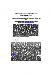
Figure 5.5: DBLP DB coauthorship graph
5000
Frequency
4000 3000 2000 1000 0 0
20
40
60
80
# Publications
Figure 5.6: Distribution of the number of DB publications (avg: 2.6, stdev: 5.1)
nodes and edges of graphs are implemented by issuing SQL queries to the PostgreSQL database. All experiments were run on a 2.8GHz Pentium 4 machine running Fedora 2, and equipped with a 250GB SATA disk. For all experiments (except the one in Section 5.4.4.3), we set the buffer pool size to 512MB and working memory size to 256MB.
118
Figure 5.7: The SNAP result for DBLP DB dataset
D1 D2 D3 D4
Description DB D1+AL D2+OS +CC D3+AI
#Nodes 7,445 14,533 22,435 30,664
#Edges 19,971 37,386 55,007 70,669
Avg. Degree 5.4 5.1 4.9 4.6
Table 5.1: The DBLP Datasets for the Efficiency Experiments
5.4.1
Experimental Datasets
In this section, we describe the datasets used in our empirical evaluation. We use two real datasets and one synthetic dataset to explore the effect of various graph characteristics. DBLP Dataset This dataset contains the DBLP Bibliography data [32] downloaded on July 30, 2007. We use this data for both effectiveness and efficiency experiments. In order to compare the coauthorship behaviors across different research areas and construct datasets for the efficiency experiments, we partition the DBLP data into different research areas. We choose the following five areas: Database (DB), Al-
119
gorithms (AL), Operating Systems (OS), Compiler Construction (CC) and Artificial Intelligence (AI). For each of the five areas, we collect the publications of a number of selected journals and conferences in this area1 . These journals and conferences are selected to construct the four datasets with increasing sizes for the efficiency experiments (see Table 5.1). These four datasets are constructed as follows: D1 contains the selected DB publications. We add into D1 the selected AL publications to form D2. D3 is D2 plus the selected OS and CC publications. And finally, D4 contains the publications of all the five areas we are interested in. We construct a coauthorship graph for each dataset. The nodes in this graph correspond to authors and edges indicate coauthorships between authors. The statistics for these four datasets are shown in Table 5.1. Political Blogs Dataset This dataset is a network of 1490 webblogs on US politics and 19090 hyperlinks between these webblogs [1] (downloaded from http: //www-personal.umich.edu/~mejn/netdata/). Each blog in this dataset has an attribute describing its political leaning as either liberal or conservative. Synthetic Dataset Most real world graphs show power-law degree distributions and small-world characteristics [37]. Therefore, we use the R-MAT model [13] in the GTgraph suites [2] to generate graphs with power-law degree distributions and small-world characteristics. Based on the statistics in Table 5.1, we set the average node degree in each synthetic graph to 5. We used the default values for the other 1
DB: VLDB J., TODS, KDD, PODS, VLDB, SIGMOD; AL: STOC, SODA, FOCS, Algorithmica, J. Algorithms, SIAM J. Comput., ISSAC, ESA, SWAT, WADS; OS: USENIX, OSDI, SOSP, ACM Trans. Comput. Syst., HotOS, OSR, ACM SIGOPS European Workshop; CC: PLDI, POPL, OOPSLA, ACM Trans. Program. Lang. Syst., CC, CGO, SIGPLAN Notices, ECOOP; AI: IJCAI, AAAI, AAAI/IAAI, Artif. Intell.
120
Attribute Only DB 0.84 P Size: 509
k=4
HP Size: 110 0.95
0.84 P Size: 509
0.29 0.91
0.48
k=5
HP Size: 110
0.95
0.84 P Size: 509
0.41 0.91
1.00
k=6
HP Size: 110
0.95 P Size: 509
1.00 0.91
0.94 0.96 LP Size: 1855 0.11
LP Size: 6826 0.84
P Size: 509
1.00 0.91
0.94
LP Size: 1855 0.75
LP Size: 1855 0.75
HP Size: 110 0.95 0.97 1.00
0.91
LP 0.01 Size: 521 0.93 0.08
0.96
0.10
LP Size: 3779 LP Size: 3047
0.84
0.94
0.22 0.80 0.19
HP Size: 110 0.95
0.96 0.75
0.22 LP Size: 3779
0.84
k=7
0.80
0.20 0.18 0.80 0.15 LP Size: 1192
LP Size: 3018
0.76
0.37 0.06 LP 0.18 1.00 0.11 Size: 761 0.14 LP Size: 1192 0.76
0.10 0.37 0.06 LP LP Size: 2497 0.980.18 0.16 0.11 Size: 761 0.08 LP Size: 1192 0.76
AI 0.54
HP Size: 76 0.92
HP 0.54 Size: 76 0.92
P Size: 545 0.80
HP 0.54 Size: 76 0.92
P Size: 545 0.80
0.37
HP 0.92 0.54 Size: 76
P Size: 545 0.80
0.99
0.54
P Size: 545 0.80 0.91 0.97
0.99
P Size: 545 0.80 0.91 0.97
0.18 LP Size: 837
LP Size: 837
0.06 0.12 0.13 LP Size: 8874 0.78
LP 0.17 Size: 5899 0.75 0.15 LP Size: 2975 0.72
0.10
0.22 LP Size: 1502 0.10
0.17 0.13 LP Size: 2975 0.72
LP Size: 4397 1.00
HP Size: 76 0.92 0.09
LP Size: 3880 0.98 0.07
0.18 0.04
0.06 0.22
0.04
LP Size: 1502 0.09
0.19 0.11 LP Size: 2138 1.00
0.10 LP Size: 4397 1.00
0.22
0.02
LP Size: 1502 0.09
0.19 LP Size: 2138
0.28
0.18 LP Size: 517
0.92
1.00
Table 5.2: The Aggregation Results for the DBLP DB and AI Subsets
parameters in the R-MAT based generator. We also assign an attribute to each node in a generated graph. The domain of this attribute has 5 values. For each node we randomly assign one of the five values.
5.4.2
Effectiveness Evaluation
We first evaluate the effectiveness of our graph summarization methods. In this section, we use only the top-down approach to evaluate the k-SNAP operation, as we compare the top-down and the bottom-up approaches in Section 5.4.3.
5.4.2.1
DBLP Coauthorship Networks
In this experiment, we are interested in analyzing how researchers in the database area coauthor with each other. As input, we use the DBLP DB subset (see D1 of 121
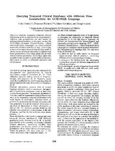
Table 5.1 and Figure 5.5). Each node in this graph has one attribute called PubNum, which is the number of publications belonging to the corresponding author. By plotting the distribution of the number of publications of this dataset in Figure 5.6, we assigned another attribute called Prolific to each author in the graph indicating whether that author is prolific: authors with ≤ 5 papers are tagged as low prolific (LP), authors with > 5 but ≤ 20 papers are prolific (P), and the authors with > 20 papers are tagged as highly prolific (HP). We first issue a SNAP operation on the Prolific attribute and the coauthorships. The result is visualized in Figure 5.7. Groups with the HP attribute value are colored in yellow, groups with the P value are colored in light blue, and the remaining groups with the attribute value LP are in white. The SNAP operation results in a summary with 3569 groups and 11293 group relationships. This summary is too big to analyze. On the other hand, if we apply the SNAP operation on only the Prolific attribute (i.e. not considering any relationships in the SNAP operation), we will get a summary with only 3 groups as visualized in the top left figure in Table 5.2. The bold edges between two groups indicate strong group relationships (with more than 50% participation ratio), while dashed edges are weak group relationships. This summary shows that the HP researchers as a whole have very strong coauthorship with the P group of researchers. Researchers within both groups also tend to coauthor with people within their own groups. However, this summary does not provide a lot of information for the LP researchers: they tend to coauthor strongly within their group and they have some connection with the HP and P groups. Now we make use of the k-SNAP operation to produce summaries with multiple 122
resolutions. The first row of figures in Table 5.2 shows the k-SNAP results for k =4, 5, 6 and 7. As k increases, more details are shown in the summaries. When k = 7, the summary shows that there are 5 subgroups of LP researchers. One group of 1192 LP researchers strongly collaborates with both HP and P researchers. One group of 521 only strongly collaborates with HP researchers. One group of 1855 only strongly collaborates with P researchers. These three groups also strongly collaborate within their groups. There is another group of 2497 LP researchers that has very weak connections to other groups but strongly cooperates among themselves. The last group has 761 LP researchers, who neither coauthor with others within their own group nor collaborate strongly with researchers in other groups. They often write single author papers. Now, in the k-SNAP result for k = 7, we are curious if the average number of publications for each subgroup of the LP researchers is affected by the coauthorships with other groups. The above question can be easily answered by applying the avg operation on the PubNum attribute for each group in the result of the k-SNAP operation. With this analysis, we find that the group of LP researchers who collaborate with both P and HP researchers has a high average number of publications: 2.24. The group only collaborating with HP researchers has 1.66 publications on average. The group collaborating with only the P researchers has on average 1.55 publications. The group that tends to only cooperate among themselves has a low average number of publications: 1.26. Finally, the group of mostly single authors has on average only 1.23 publications. Not surprisingly, these results suggest that collaborating with HP 123
and P researchers is very helpful for the low prolific (often beginning) researchers. Next, we want to compare the database community with the AI community to see whether the coauthorship relationships are different across these two communities. We constructed the AI coauthorship graph with 9495 authors and 16070 coauthorships from the DBLP AI subset. The distribution of the number of publications of AI authors is similar to the DB authors, thus we use the same method to assign the Prolific attribute to these authors. The SNAP operation on the Prolific attribute and coauthorships results in a summary with 3359 groups and 7091 group relationships. The second row of figures in Table 5.2 shows the SNAP result based only on the Prolific attribute and the k-SNAP results for k =4, 5, 6 and 7. Comparing the summaries for the two communities for k = 7, we can see the differences across the two communities: The HP and P groups in the AI community have a weaker cooperation than the DB community; and there isn’t a large group of LP researchers who strongly coauthor with both HP and P researchers in the AI area. As this example shows, by changing the resolutions of summaries, users can better understand the characteristics of the original graph data and also explore the differences and similarities across different datasets.
5.4.2.2
Political Blogs Network
In this experiment, we evaluate the effectiveness of our graph summarization methods on the political blogs network (1490 nodes and 19090 edges). The SNAP operation based on the political leaning attribute and the links between blogs results in a summary with 1173 groups and 16657 group relationships. The SNAP result based 124
Attribute Only L Size: 758
k=7 L Size: 320
0.76 L Size: 245
0.95
0.86 0.51
0.09 L Size: 193
C Size: 128
0.42 C Size: 732
C Size: 96
0.01
1.00 0.56
0.86
C Size: 303
0.89
C Size: 205
1.00
0.97
Delta/k
Table 5.3: Aggregation results for Political Blogs Dataset 1100 1000 900 800 700 600 500 400 300 200 100 0
TopDown BottomUp
8
16
32
64
128
256
512 1024 20483569
k (log scale)
Figure 5.8: Quality of summaries: top-down vs. bottom-up
only on the attribute and the k-SNAP result based on both the attribute and the links for k = 7 are shown in Table 5.3. From the results, we see that there are a group of liberal blogs and a group of conservative blogs that interact strongly with each other (perhaps to refute each other). Other groups of blogs only connect to blogs in their own communities (liberal or conservative), if they do connect to other blogs. There is a relatively large group of 193 liberal blogs with almost no connections to any other blogs, while such isolated blogs compose a much smaller portion (96 blogs) of all the conservative blogs. Overall, conservative blogs show a slightly higher tendency to link with each other than liberal
125
Execution Time (sec, log scale)
16000 5000
500
TopDown BottomUp
50 5 1 8
16
32
64
128
256
512 1024 20483569
k (log scale)
Figure 5.9: Efficiency: top-down vs. bottom-up
blogs, which is consistent with the conclusion from the analysis in [1]. Given that the blogs data was collected right after the US 2004 election, the authors in [1] speculated that the different linking behaviors in the two communities may be correlated with eventual outcome of the 2004 election.
5.4.3
k-SNAP: Top-Down vs. Bottom-Up
In this section, we compare the top-down and the bottom-up k-SNAP algorithms, both in terms of effectiveness and efficiency. We use the DBLP DB subset (D1 in Table 5.1) and apply both approaches for different k values. For the effectiveness experiment, we use the ∆ measure introduced in Section 5.2.2 to assess the qualities of summaries. Note that for a given k value, smaller ∆ value means better quality summary, but for different k values, comparing ∆ does not make sense, as a higher k value tends to result in a higher ∆ value according to Equation V.1. However, if we normalize ∆ by k, we get the average contribution of each group to the ∆ value, then we can compare
126
∆ k
for different k values.
We acknowledge that
∆ k
is not a perfect measure for “quantitatively” evaluating
the quality of summaries. However, quality assessment is a tricky issue in general, and
∆ , k
though crude, is an intuitive measure for this study.
Figure 5.8 shows the comparison of the summary qualities between the top-down and the bottom-up approaches. Note that the x-axis is in log scale and the y-axis is ∆ . k
First, as k increases, both methods produce higher quality summaries. For small
k values, top-down approach produces significantly higher quality summaries than the bottom-up approach. This is because, the bottom-up approach starts from the grouping produced by the SNAP operation. This initial grouping is usually very large, in this case, it contains 3569 groups. The bottom-up approach has to continuously merge groups until the number of groups decreases to a small k value. Each merge decision is only made based on the current grouping, and errors can easily accumulate. In contrast, the top-down approach starts from the maximum A-compatible grouping, and only needs a small number of splits to reach the result. Therefore, small amount of errors is accumulated. As k becomes larger, the bottom-up approach shows slight advantage over the top-down approach. The execution times for the two approaches are shown in Figure 5.9. Note that both axes are in log scale. The top-down approach significantly outperform the bottom-up approach, except when k is equal to the size of the grouping resulting from the SNAP operation. Initializing the heap takes a lot of time for the bottom-up approach, as it has to compare every pair of groups. This situation becomes worse, if the size of the initial grouping is very large. In practice, users are more likely to choose small k values to generate summaries. 127
D1 D2 D3 D4
# Groups 3569 7892 11379 15052
# Group Relationships 11293 26031 35682 44318
Time(sec) 6.4 16.1 27.9 44.0
Table 5.4: The SNAP Results for the DBLP Datasets
The top-down approach significantly outperforms the bottom-up approach in both effectiveness and efficiency for small k values. Therefore, the top-down approach is preferred for most practical uses. For all the remaining experiments, we only consider the top-down approach.
5.4.4
Efficiency Experiment
This section evaluates the efficiency the SNAP and the k-SNAP operations.
5.4.4.1
SNAP Efficiency
In this section, we apply the SNAP operation on the four DBLP datasets with increasing sizes (see Table 5.1). Table 5.4 shows the number of groups and group relationships in the summaries produced by the SNAP operation on the attribute Prolific (defined in the same way as in Section 5.4.2.1) and coauthorships, as well as the execution times. Even for the largest dataset with 30664 nodes and 70669 edges, the execution is completed in 44 seconds. However, all of the SNAP results are very large. The summary sizes are comparable to the input graphs. Such large summaries are often not very useful for analyzing the input graphs. This is an anecdotal evidence of why the k-SNAP operation is often more desired than the SNAP operation in
128
Runing Time (sec)
250
D1
200
D2
D3
D4
150 100 50 0 8
16
32
64
128
256
512
1024
2048
3569
k
Execution Time (sec)
Figure 5.10: Efficiency experiment for DBLP datasets
10000 9000 8000 7000 6000 5000 4000 3000 2000 1000 0
k=10 k=100 k=1000
50k
200k
500k
800k
1000k
Graphs Sizes (#nodes)
Figure 5.11: Efficiency experiment for synthetic datasets
practice.
5.4.4.2
k-SNAP Efficiency
This section evaluates the efficiency of the top-down k-SNAP algorithm on both the DBLP and the synthetic datasets. DBLP Data In this experiment, we apply the top-down k-SNAP evaluation algorithm on the four DBLP datasets shown in Table 5.1 (the k-SNAP operation is based on Prolific attribute and coauthorships). The execution times with increasing graph sizes and increasing k values are shown in Figure 5.10. For these datasets, the 129
Execution Time (sec)
2000 1500
No Bitmap Bitmap in Memory
1000 500 0 0
1000
2000
3000
k
Figure 5.12: Bitmap in memory vs. no bitmap
performance behavior is close to linear, since the execution times are dominated by the database page accesses (as discussed in Section 5.3.3.1). Synthetic Data We apply the k-SNAP operation on different sized synthetic graphs with three k values: 10, 100 and 1000. The execution times with increasing graph sizes are shown in Figure 5.11. When k = 10, even on the largest graph with 1 million nodes and 2.5 million edges, the evaluation algorithm finishes in about 5 minutes. For a given k value, the algorithm scales nicely with increasing graph sizes.
5.4.4.3
Evaluation with Very Large Graphs
So far, we have assumed that the amount of working memory is big enough to hold all the data structures (shown in Figure 5.4) used in the evaluation algorithms. This is often the case in practice, as large multi GB memory configurations are common and many graph datasets can fit in this space (especially if a subset of large graph is selected for analysis). However, our methods also work, when the graph datasets are extremely large and this in-memory assumption in not valid. In this section, we discuss the behaviors of our methods for this case. We only consider the most 130
practically useful top-down k-SNAP algorithm for this experiment. In the case when the most memory consuming data structure, namely the neighborgroups bitmap (see Figure 5.4), cannot fit in memory, the top-down approach drops the bitmap data structure. Without the bitmap, each time the algorithm splits a group, it has to query the edges information in the database to infer the neighborgroups. We have implemented a version of the top-down k-SNAP algorithm without the bitmap data structure, and compared it with the normal top-down algorithm. To keep this experiment manageable, we scaled down the experiment settings. We used the DBLP D4 dataset in Table 5.1, and set the buffer pool size and working memory size to 16MB and 8MB, respectively. This “scaled-down” experiment exposes the behaviors of the two versions of the top-down algorithm, while keeping the running times reasonable. As shown in Figure 5.12, the version of the top-down approach without bitmap is much slower than the normal version. This is not surprising as the former incurs more disk IOs. Given the graph size and the k value, our current implementation can decide in advance whether the bitmap can fit in the working memory, by estimating the upper bound of the bitmap size. It can then choose the appropriate version of the algorithm to use. In the future, we plan on designing a more sophisticated version of the top-down algorithm in which part of the bitmap can be kept in memory when the available memory is small.
131
5.5
Conclusions
This chapter has introduced two aggregation operations SNAP and k-SNAP for controlled and intuitive database-style graph summarization. Our methods allow users to freely choose node attributes and relationships that are of interest, and produce summaries based on the selected features. Furthermore, the k-SNAP aggregation allows users to control the resolutions of summaries and provides “drill-down” and “roll-up” abilities to navigate through the summaries. We have formally defined the two operations and proved that evaluating the k-SNAP operation is NP-complete. We have also proposed an efficient algorithm to evaluate the SNAP operation and two heuristic algorithms to approximately evaluate the k-SNAP operation. Through extensive experiments on a variety of real and synthetic datasets, we show that of the two k-SNAP algorithms, the top-down approach is a better choice in practice. Our experiments also demonstrate the effectiveness and efficiency of our methods. As part of future work, we plan on designing a formal graph data model and query language that allows incorporation of k-SNAP, along with a number of other additional common and useful graph matching methods.
132
CHAPTER VI Related Work
6.1
Graph Matching Methods
There is a long history of database research on methods for querying graphs. However, most previous works have focused on exact graph or subgraph matching, i.e. graph or subgraph isomorphism. Subgraph isomorphism was proved to be NPcomplete in [19]. Ullmann [51] proposed a subgraph matching algorithm based on a state space search method with backtracking. However, this algorithm is prohibitively expensive for querying against database with a large number of graphs. To reduce the search space, GraphGrep [45], GIndex [58] and TreePi [61] index substructures of the database (paths, frequent subgraphs and trees respectively) to filter out graphs that do not match the query. Several index-based methods for approximate subgraph matching have also been proposed. However, most of these techniques only apply to small graphs and allow limited approximation. Grafil [59] and PIS [60] are both built on top of the exact
133
subgraph matching method GIndex. However, neither method allows node insertion or deletion in their match models. CDIndex [55] only applies to graphs with limited sizes, as it exhaustedly enumerates and indexes all the subgraphs in the database. GString [28] utilizes sequence matching to answer graph queries, but it only applies to applications in which the graphs contain a small number of basic substructures. C-Tree [22], which employs an R-tree like index structure, is a more general tool than the above methods. However, C-Tree, as well as Grafil, PIS, CDIndex and GString, utilize memory-based indexing techniques, which require the indexes to be memory resident during query processing. As the database size increases, these indexes quickly grow out of memory. On the contrary, the indexing approaches in SAGA and TALE are disk-based. The life science community has produced vast amount of protein interaction networks. Several tools for comparing protein interaction networks have been proposed. These include PathBlast [30], its successor NetworkBlast [40], MaWIsh [35], and Graemlin [17]. Of these, Graemlin is the latest method and in many ways superior to the other methods for comparing protein interaction networks.
6.2
Graph Summarization Methods
Graph summarization has attracted a lot of interest from both the sociology and the database research communities. Most existing works on graph summarization use statistical methods to study graph characteristics, such as degree distributions, hop-plots and clustering coefficients. Comprehensive surveys on these methods are
134
provided in [11] and [37]. A-plots [12] is a novel statistical method to summarize the adjacency matrix of graphs for outlier detection. Statistical summaries are useful but hard to control and navigate. Methods for mining frequent graph patterns [26, 52, 57] are also used to understand the characteristics of large graphs. Washio and Motoda [53] provide an elegant review on this topic. However, these mining algorithms often produces an overwhelmingly large number of frequent patterns. Various graph partitioning algorithms [38, 48, 56] are used to detect community structures (dense subgraphs) in large graphs. SuperGraph [43] employs hierarchical graph partitioning to visualize large graphs. In [7], Frey and Dueck proposed a novel clustering method by passing messages between nodes in the graph. However, graph partitioning or clustering techniques largely ignore the node attributes in the summarization. Studies on graph visualization are surveyed in [3, 23]. For very large graphs, these visualization methods are still not enough. Unlike these existing methods, we introduce two database-style operations to summarize large graphs. Our method allows users to easily control and navigate through summaries. Previous research [4, 6, 41] have also studied the problem of compressing large graphs, especially Web graphs. However, these graph compression methods mainly focus on compact graph representation for easy storage and manipulation, whereas graph summarization methods aim at producing small and understandable summaries. Regular equivalence is introduced in [54] to study social roles of nodes based on graphs structures in social networks. It shares resemblance with the SNAP operation. However, regular equivalence is defined only based on the relationships between nodes. 135
Node attributes are largely ignored. In addition, the k-SNAP operation relaxes the stringent equivalence requirement of relationships between node groups, and produces user controllable multi-resolution summaries. The SNAP algorithm shares similarity with the automorphism partitioning algorithm in [16]. However, the automorphism partitioning algorithm only partitions nodes based on node degrees and relationships, whereas SNAP can be evaluated based on arbitrary node attributes and relationships that a user selects.
136
CHAPTER VII Conclusions
The rapidly growing graph datasets have made graph querying systems critical for many modern applications. To allow users to perform complex analysis on graph data, this thesis develops a graph querying toolkit, called Periscope/GQ. This toolkit provides a uniform schema for storing graphs in the database and supports various graph query operations, especially sophisticated query operations. Approximate graph matching query is one of the sophisticated query operations that Periscope/GQ supports, due to its usefulness and advantage over the exact graph matching query. Chapter III introduces an efficient approximate graph matching method, called SAGA. SAGA employs a flexible graph similarity model and an indexbased matching algorithm to efficiently evaluate approximate graph matching queries. To further handle the case of large query graphs, Chapter IV proposes another approximate graph matching technique TALE. TALE utilizes a novel indexing technique, which achieves high pruning power and linear index size with the database size. The TALE matching algorithm first uses the index to match the important nodes in
137
the query, and then progressively extends these matches. Chapter V proposes two aggregation operations for efficient graph summarization. The SNAP operation, produces a summary graph by grouping nodes based on userselected node attributes and relationships. The k-SNAP operation allows users to further control the resolutions of summaries and provides the “drill-down” and “rollup” abilities to navigate through summaries with different resolutions. Extensive experiments on a variety of real applications have demonstrated the effectiveness and efficiency of the Periscope/GQ toolkit.
138
APPENDICES
139
APPENDIX A Statistical Evaluation for Approximate Graph Matching Results
In many applications, especially life sciences applications, producing the approximate graph matching results is not enough. It is also very important to evaluate the statistical significance of the matching results, i.e. assess whether an approximate graph match constitutes a meaningful result or a random accident. Periscope/GQ employs the Monte Carlo simulation approach to evaluate the statistical significance of the matches for general applications. However, this approach brings significant computation overhead. Making use of domain knowledge, experts can develop more light-weight statistical evaluation methods. As an anecdotal example, we introduce a specific statistical scoring model designed for the application of matching parsed literature graphs (see Section 3.3.4 of Chapter III).
140
1.1
Monte Carlo Simulation
The Monte Carlo simulation approach relies on matching a query against random graphs to estimate the p-value of a query result (the probability of obtaining a result at least as good as the one that was actually observed by change). Periscope/GQ generates random graphs by randomly shuffling edges of the graphs in the database preserving the node degrees, and randomizing the orthologous groups of each node preserving the number of orthologous groups that each node belongs to. For a given query, in addition to querying the real database, the query is also run against a large number of random graphs. A p-value of a match from the real database is estimated as the fraction of matches from the random graphs with the same or a larger size (in number of nodes) and the same or a better similarity value (e.g. SAGA graph distance value).
1.2
An Application Specific Statistical Scoring Model
For the application of matching parsed literature graphs (see Section 3.3.4 of Chapter III), we developed a light-weight method to assess the statistical significance based on domain knowledge. This method does not need any simulation on random graphs. Instead, it can be simply calculated based on the query graph, the target graph and the match, thus significantly speeds up the statistical evaluation. The statistical score for a query to a target graph in the database is defined as follows: S = −log(P (Nme |Nmn ) ∗ P (Nmn )) 141
Notation Ng Nn Nmn Ne Nme
Description The total number of genes in a species The number of nodes in the target graph The number of matching nodes in the target graph The number of edges connecting the matching nodes in the target graph The number of matching edges in the target graph
Table 1.1: The Notation Table
In the above equation, Nmn is the number of matching nodes, Nme is the number of matching edges, P (Nmn ) is the probability of selecting Nmn matching nodes at random from the target graph, and P (Nme |Nmn ) is the probability of selecting Nme matching edges given Nmn matching nodes. Table 1.1 lists the descriptions of the notations used in the computation of this statistical scoring method.
1.2.1
Calculating P (Nmn )
P (Nmn ) is the probability of selecting Nmn matching nodes at random from the target graph. Assume that all nodes, which represent genes in this application, are equally likely to be matched, and there are Ng genes in a typical genome (Ng = 20,000 in general). For a target graph, containing Nn nodes and matching Nmn of these with the query, the number of ways to choose the Nmn matching nodes in the target is Ncn = Nn !/(Nmn ! ∗ (Nn − Nmn )!). And the number of ways to choose Nmn nodes (or genes) from the genome is Ncg = Ng !/(Nmn ! ∗ (Ng − Nmn )!). Therefore, the probability that the matching nodes are selected at random is P (Nmn ) = Ncn /Ncg .
142
1.2.2
Calculating P (Nme |Nmn )
P (Nme |Nmn ) is the probability of selecting Nme matching edges given Nmn matching nodes. Let Ne be the number of edges connecting the Nmn matching nodes in the target graph. Assume that each edge from the Ne edges are equally likely to be selected as a matching edge (Pe = 1/Ne ). The number of ways to choose Nme matching edges is Nce = (Ne !/(Nme ! ∗ (Ne − Nme )!). The probability that there are Nme matching edges given Nmn matching nodes is P (Nme |Nmn ) = Nce ∗ PeNme (The chance that an edge is in the matching set raised to the power of number of edges multiplied by the number of ways to choose the matching set from the set of possible edges).
143
BIBLIOGRAPHY
144
BIBLIOGRAPHY
[1] L. A. Adamic and N. Glance. The political blogosphere and the 2004 us election. In WWW Workshop on the Weblogging Ecosystem, 2005. [2] D. A. Bader and K. Madduri. GTgraph: A suite of synthetic graph generators. http://www.cc.gatech.edu/~kamesh/GTgraph. [3] G. Battista, P. Eades, R. Tamassia, and I. Tollis. Graph Drawing: Algorithms for the Visualization of Graphs. Prentice Hall, 1999. [4] D. K. Blandford, G. E. Blelloch, and I. A. Kash. Compact representations of separable graphs. In Proceedings of SODA’03, pages 679–688, 2003. [5] B. H. Bloom. Space/time trade-offs in hash coding with allowable errors. Commun. ACM, 13(7):422–426, 1970. [6] P. Boldi and S. Vigna. The WebGraph framework I: Compression techniques. In Proceedings of WWW’04, pages 595–602, 2004. [7] F. Brendan J and D. Dueck. Clustering by passing messages between data points. Science, 315:972–976, 2007.
145
[8] C. Bron and J. Kerbosch. Algorithm 457: finding all cliques of an undirected graph. CACM, 16(9):575–577, 1973. [9] H. Bunke. On a relation between graph edit distance and maximum common subgraph. Pattern Recogn. Lett., 18(8):689–694, 1997. [10] C. Alfarano et al. The biomolecular interaction network database and related tools 2005 update. Nucleic Acids Res., 33:D418–D424, 2005. [11] D. Chakrabarti and C. Faloutsos. Graph mining: Laws, generators, and algorithms. ACM Comput. Surv., 38(1), 2006. [12] D. Chakrabarti, C. Faloutsos, and Y. Zhan. Visualization of large networks with min-cut plots, A-plots and R-MAT. Int. J. Hum.-Comput. Stud., 65(5), 2007. [13] D. Chakrabarti, Y. Zhan, and C. Faloutsos. R-MAT: A recursive model for graph mining. In SDM, 2004. [14] M. Chen and R. Hofestaedt. Applied Bioinformatics, 3(4):241–252, 2004. [15] A. Coppen.
The biochemistry of affective disorders.
Br J Psychiatry,
113(504):1237–64, 1967. [16] D. G. Corneil and C. C. Gotlieb. An efficient algorithm for graph isomorphism. J. ACM, 17(1):51–64, 1970. [17] J. Flannick, A. Novak, B. S. Srinivasan, H. H. McAdams, and S. Batzoglou. Græmlin: General and robust alignment of multiple large interaction networks. Genome Res., 16:1169–1181, 2006. 146
[18] G. Joshi-Tope et al. Reactome: a knowledgebase of biological pathways. Nucleic Acids Res., 33:D428–32, 2005. [19] M. R. Garey and D. S. Johnson. Computers and Intractability: A Guide to the Theory of NP-Completeness. W. H. Freeman & Co., New York, NY, USA, 1979. [20] R. Giugno and D. Shasha. Graphgrep: A fast and universal method for querying graphs. In IEEE International Conference in Pattern recognition, 2002. [21] R. H. Guting. Graphdb: Modeling and querying graphs in databases. In VLDB, pages 297–308, 1994. [22] H. He and A. K. Singh. Closure-tree: an index structure for graph queries. In ICDE, 2006. [23] I. Herman, G. Melan¸con, and M. S. Marshall. Graph visualization and navigation in information visualization: A survey. IEEE Trans. Vis. Comput. Graph., 6(1), 2000. [24] D. S. Hochbaum. Approximation Algorithms for NP-Hard Problems. PWS Publishing Co., Boston, 1997. [25] J. Hu, X. Shen, Y. Shao, C. Bystroff, and M. J. Zaki. Mining protein contact maps. In BIOKDD, 2002. [26] J. Huan, W. Wang, J. Prins, and J. Yang. Spin: mining maximal frequent subgraphs from graph databases. In KDD, 2004.
147
[27] J. Chandonia et al.
The astral compendium in 2004.
Nucleic Acids Res.,
32:D189–D192, 2004. [28] H. Jiang, H. Wang, P. S. Yu, and S. Zhou. Gstring: A novel approach for efficient search in graph databases. In ICDE, 2007. [29] D. Kalderon. Similarities between the hedgehog and wnt signaling pathways. Trends in Cell Biology, 12(11):523–531, 2002. [30] B. P. Kelley, B. Yuan, F. Lewitter, R. Sharan, B. R. Stockwel, and T. Ideker. Pathblast: a tool for alignment of protein interaction networks. Nucleic Acids Res., pages W83–W88, 2004. [31] M. Koyuturk, A. Grama, and W. Szpankowski. Pairwise local alignment of protein interaction networks guided by models of evolution. In International Conference on Research in Computational Molecular Biology, pages 48–65, 2005. [32] M. Ley. DBLP Bibliography. http://www.informatik.uni-trier.de/~ley/ db/. [33] W. Li, L. Jaroszewski, and A. Godzik. Clustering of highly homologous sequences to reduce the size of large protein database. Bioinformatics, 17:282–283, 2001. [34] M. Kanehisa et al. The kegg resources for deciphering the genome. Nucleic Acids Res., 32:D277–D280, 2004. [35] M. Koyuturk et al. Pairwise alignment of protein interaction networks. Journal of Computational Biology, 13(2):182–199, 2006. 148
[36] M. Tourigny et al. Cdk inhibitor p18ink4c is required for the generation of functional plasma cells. Immunity, 17(2):179–189, 2002. [37] M. E. J. Newman. The structure and function of complex networks. SIAM Review, 45, 2003. [38] M. E. J. Newman and M. Girvan. Finding and evaluating community structure in networks. Physical Review E, 69, 2004. [39] R. Nusse. Wnts and hedgehogs: lipid-modified proteins and similarities in signaling mechanisms at the cell surface. Development, 130:5297–5305, 2003. [40] R. Sharan et al. Conserved patterns of protein interaction in multiple species. PNAS, 102:1974–1979, 2005. [41] S. Raghavan and H. Garcia-Molina. Representing Web graphs. In Proceedings of ICDE’03, pages 405–416, 2003. [42] F. S. Roberts and L. Sheng. How hard is it to determine if a graph has a 2-role assignment? Networks, 37(2), 2001. [43] J. F. Rodrigues, A. J. M. Traina, C. Faloutsos, and C. T. Jr. SuperGraph visualization. In ISM, 2006. [44] G. Salton and M. McGill.
Introduction to Modern Information Retrieval.
McGraw-Hill, New York, 1983. [45] D. Shasha, J. T.-L. Wang, and R. Giugno. Algorithmics and applications of tree and graph searching. In PODS, 2002. 149
[46] L. Sheng, Z. M. Ozsoyoglu, and G. Ozsoyoglu. A graph query language and its query processing. In ICDE, 1999. [47] E. Sprinzak, S. Sattath, and H. Margalit. How reliable are experimental proteinprotein interaction data? Journal of Molecular Biology, 327(5):919–923, 2003. [48] J. Sun, Y. Xie, H. Zhang, and C. Faloutsos. Less is more: Compact matrix decomposition for large sparse graphs. In SDM, 2007. [49] T. Luedde et al. p18(ink4c) collaborates with other cdk-inhibitory proteins in the regenerating liver. Hepatology, 37(4):833–841, 2003. [50] R. L. Tatusov, E. V. Koonin, and D. J. Lipman. A genomic perspective on protein families. Science, 278(5388):631–7, 1997. [51] J. R. Ullmann. An algorithm for subgraph isomorphism. J. ACM, 23(1):31–42, 1976. [52] W. Wang, C. Wang, Y. Zhu, B. Shi, J. Pei, X. Yan, and J. Han. Graphminer: a structural pattern-mining system for large disk-based graph databases and its applications. In SIGMOD, 2005. [53] T. Washio and H. Motoda. State of the art of graph-based data mining. SIGKDD Explor. Newsl., 5(1), 2003. [54] D. R. White and K. P. Reitz. Graph and semigroup homomorphisms on semigroups of relations. Social Networks, 1983.
150
[55] D. Williams, J. Huan, and W. Wang. Graph database indexing using structured graph decomposition. In ICDE, 2007. [56] X. Xu, N. Yuruk, Z. Feng, and T. A. J. Schweiger. SCAN: a structural clustering algorithm for networks. In KDD, 2007. [57] X. Yan and J. Han. gspan: Graph-based substructure pattern mining. In ICDM, 2002. [58] X. Yan, P. S. Yu, and J. Han. Graph indexing: a frequent structure-based approach. In SIGMOD, 2004. [59] X. Yan, P. S. Yu, and J. Han. Substructure similarity search in graph databases. In SIGMOD, 2005. [60] X. Yan, F. Zhu, J. Han, and P. S. Yu. Searching substructures wuth superimposed distance. In ICDE to appear, 2006. [61] S. Zhang, M. Hu, and J. Yang. Treepi: A new graph indexing method. In ICDE, 2007.
151