dential Reunion' and 'How the Grinch Stole Christmas!', as the best answer, which corresponds to the fact in real life. These results illustrate that our algorithm ...
Querying Web-Scale Information Networks Through Bounding Matching Scores Jiahui Jin†‡ , Samamon Khemmarat‡ , Lixin Gao‡ , Junzhou Luo†
†
‡
School of Computer Science and Engineering, Southeast University, China Department of Electrical and Computer Engineering, University of Massachusetts Amherst, USA
{jhjin, jluo}@seu.edu.cn; {khemmarat, lgao}@ecs.umass.edu ABSTRACT
1.
Web-scale information networks containing billions of entities are common nowadays. Querying these networks can be modeled as a subgraph matching problem. Since information networks are incomplete and noisy in nature, it is important to discover answers that match exactly as well as answers that are similar to queries. Existing graph matching algorithms usually use graph indices to improve the efficiency of query processing. For web-scale information networks, it may not be feasible to build the graph indices due to the amount of work and the memory/storage required. In this paper, we propose an efficient algorithm for finding the best k answers for a given query without precomputing graph indices. The quality of an answer is measured by a matching score that is computed online. To speed up query processing, we propose a novel technique for bounding the matching scores during the computation. By using bounds, we can efficiently prune the answers that have low qualities without having to evaluate all possible answers. The bounding technique can be implemented in a distributed environment, allowing our approach to efficiently answer the queries on web-scale information networks. We demonstrate the effectiveness and the efficiency of our approach through a series of experiments on real-world information networks. The result shows that our bounding technique can reduce the running time up to two orders of magnitude comparing to an approach that does not use bounds.
Information networks such as Freebase [12] have become massive in recent years. Freebase, a collaborative knowledge graph, contains more than 43.9 million entities, interconnected by 2.4 billion facts. The Linked Open Data project [4] connects RDF datasets on the web, resulting in an information network containing 1.77 billion RDF triples. It is important to be able to extract information from these networks. However, performing query operations on such web-scale information networks can be challenging. In this paper, we study the problem of identifying a set of unknown entities in an information network given a set of related entities and facts/relations. For example, a query on Freebase can be “find an actor who collaborated with the director of the movie ‘Avatar’ and also performed in the movie ‘Body of Lies’ ”. We can model an information network or a query as a graph that consists of entities and relationships (or facts) between entities. Answering queries on information networks then becomes a subgraph matching problem. While it is common to seek answers that match exactly to queries, it is equally important to discover an answer that is similar to the queries. Information networks are typically crawled from the web or a large collection of databases. Therefore, they can be incomplete and noisy. Further, a user might not know the schema of the information network well enough to specify a query. It is likely that a user describes a vague query that is similar in structure to the desired answer. Fig. 1(a) shows the query graph for the aforementioned example query. An answer to the query from Freebase, that the actor is DiCaprio and the director is Cameron, is shown in Fig. 1(b). Clearly, the answer is not an exact match to the query. In particular, actor DiCaprio does not connect to director Cameron or the movie ‘Body of Lies’ directly in Freebase. Nevertheless, this is a good answer to the query. Therefore, it is crucial to be able to identify both exact and similar matches to a query for information networks. The problem of subgraph matching has been studied extensively in the past decades [30, 28, 18, 19]. However, most of them utilize graph indices that require precomputation and storage size of super-linear to information network size [27]. It may be infeasible to build the graph indices for web-scale networks due to the amount of work and the memory/storage required. To address this problem, we propose an index-free approach for answering information queries. Our approach is able to identify all answers that have the same structure as the query as well as answers that are similar to the query. The quality of an answer is measured by
Categories and Subject Descriptors H.2.8 [Database Management]: Database Applications— graph database; C.2.4 [Computer-Communication Networks]: Distributed Systems—distributed applications
General Terms Algorithms, Design, Performance
Keywords Subgraph Matching, Graph Similarity, Billion-Node Graphs, Index-Free, Query Processing, Distributed System
Copyright is held by the International World Wide Web Conference Committee (IW3C2). IW3C2 reserves the right to provide a hyperlink to the author’s site if the Material is used in electronic media. WWW 2015, May 18–22, 2015, Florence, Italy. ACM 978-1-4503-3469-3/15/05. http://dx.doi.org/10.1145/2736277.2741131.
527
INTRODUCTION
‘Body of Lies’ Roger
‘Body of Lies’ (film)
‘Avatar’ (film)
(film)
2.
‘Avatar’ (film)
(role)
2.1
(perform)
DiCaprio ? (actor)
?
(director)
(director)
(a) Query
Jack
‘Titanic’
(role)
(film)
Preliminaries
We model an information network as a typed graph. A typed graph (V, E, T ) is an undirected graph, where V is a set of nodes, E is a set of edges, and T is a set of node types. Each node v has a node type and a name that is a string. Generally, there are many nodes having the same node type, but a node name is usually unique or shared by only a few nodes. For simplicity, we assume the node names are unique and there are no types on the edges. However, our approach can be extended for graphs with shared names and typed edges. We represent an information network by a data graph G = (VG , EG , T ) and refer to its nodes as data nodes. A query on an information graph aims to discover a set of unknown entities by providing related entities, or known entities. We model the query as a typed graph, Q = (VQ , EQ , T ). In the query graph, there are two types of nodes: (1) A specific node corresponds a known entity. Both the type and the name of a specific node are known. (2) A query node corresponds to an unknown entity. Only its type is known. In the query graph in Fig. 1, ‘Avatar’ and ‘Body of Lies’ are the specific nodes, and the two nodes with type actor and type director are the query nodes. We denote the set of specific nodes by VQS and the set of queries nodes by VQU . To answer a query, we need to map every query node to a data node. The mapping is referred to as an embedding.
Cameron
(perform)
(actor)
PROBLEM DEFINITION
(b) Answer from Freebase
Figure 1: A query on an information network
a matching score evaluated by comparing the structural signatures of the answer with that of the query. In contrast to the existing approaches, we compute matching scores online instead of precomputing the scores. To speed up query processing, we propose GraB (Graph Matching using Bound), a novel technique for bounding the matching scores during the computation. By using the bounds, we can efficiently prune the low quality answers without evaluating all the possible answers. While we present the bounding technique in the context of a specific matching score function, it can be broadly applied to other functions as well. Furthermore, we implement the bounding technique in a distributed environment. Therefore, our approach can scale to answer the queries on web-scale information networks. The key contributions of this paper are summarized as follows: • We propose an algorithm for finding the k best answers. The algorithm can be applied to identify both exact and similar matches. The algorithm uses a novel heuristic to select only the promising candidates of the unknown entities, using the known entities as guides. • In order to scale the algorithm to billions of nodes, we propose an index-free algorithm that computes matching scores online. Our index-free algorithm does not make assumptions about the extent of similarity between a query and the answers. Therefore, it is able to identify the top-k answers for every query. A novel technique for bounding the matching scores is used to efficiently find the top-k best answers. • We implement our algorithm in a distributed environment. To evaluate the scalability, we deploy the distributed system on an Amazon EC2 cluster that contains hundreds of machines. The results show that our system can support querying on graphs with billions of nodes and scale to large queries. • Our evaluation using real-world datasets shows that our algorithm can identify the top-k answers for every query and the answers are accurate. Additionally, our bounding technique can reduce the running time up to two orders of magnitude comparing to an approach that does not use bounds. The rest of this paper is organized as follows. Section 2 describes the definition of the graph similarity matching problem. Section 3 provides the framework of our algorithm. In Section 4 an index-free algorithm is proposed. Section 5 discusses our distributed solution. In Section 6, we present the evaluation of our algorithm. We discuss related work in Section 7 and conclude the paper in Section 8.
Definition 1 (Embedding). Given a data graph G and a query graph Q, an embedding of Q in G is an injective function f : VQ → VG where (1) ∀q ∈ VQ , q and f (q) have the same type; (2) ∀q s ∈ VQS , q s and f (q s ) have the same name. The embeddings that result in the subgraphs with the same structure as the query graph are exact matches. Formally, we have the following definition. Definition 2 (Exact Match). An embedding f is an exact match of a query graph Q iff for each edge (qi , qj ) ∈ EQ , there is an edge (f (qi ), f (qj )) ∈ EG . Considering the noisiness and incompleteness of the information networks, to answer a given query we are interested in finding both the exact matches and similar matches. Therefore, we consider the top-k graph similarity matching problem, which returns the best k embeddings according to a similarity measure, as described in the next section.
2.2
Similarity Measure
In this section, we propose a similarity measure to quantify the structural similarity between a query graph and an embedding. First, we introduce a closeness vector, which is used to represent a structural signature of a node’s neighborhood in a graph. The closeness vector captures the graph structure around a node using the closeness between the node and the other nodes. For a node qi in a query graph, its closeness vector specifies how close it is to each node in the query graph, defined formally as follows. Let the nodes in a query graph Q be q1 , ..., qm . The closeness vector of qi , denoted by RQ (qi ), is defined as RQ (qi ) = [ϕQ (qi , q1 ), ..., ϕQ (qi , qm )],
where ϕQ (qi , qj ) is a closeness score between qi and qj .
528
Notation VQU VQS qs φ(q s )
We design our closeness score function, which quantifies the closeness between two nodes, by aiming for two properties. (1) The closer the nodes are in terms of the shortest path distance, the higher the score. (2) When two pairs of nodes have the same shortest path distance, the pair having more shortest paths has a higher score. Based on these properties, the closeness between node u and v in a graph G, denoted by ϕG (u, v), is defined by: ( ϕG (u, v) =
1, min{nu,v αlu,v , N αlu,v },
u=v otherwise
ϕG (u, v) ϕQ (qi , qj ) δqi ,qj (u, v) C(f ) C K (v, q)
(1)
Mq F
where lu,v and nu,v are the length and the number of shortest paths between u and v, α is a constant between 0 and 1, and N is a constant smaller than α1 . When nu,v > N , the closeness score of u and v is bounded to N αlu,v , which guarantees Property (1) since N αlu,v < αlu,v −1 . To quantify the similarity between a query graph and an embedding, we also represent a match of a query node in an embedding with a closeness vector. The closeness vector of a match specifies how close it is to the other matches in the data graph. Formally, the closeness vector RG (qi , f ) of a match of qi in embedding f is defined as
Table 1: Frequently used notations nected by the edge having the same type. Otherwise, the cost of matching the edge types should be added to the embedding matching costs. Based on the defined match costs, the top-k graph similarity matching problem is defined as follows. The top-k similarity matching problem. Given a data graph G and a query graph Q, identify k embeddings that have the smallest match costs. To simplify the notation, in the rest of the paper, we let δqi ,qj (u, v) denote Θ(ϕQ (qi , qj ), ϕG (u, v)). We list the frequently used notations in Table 1.
RG (qi , f ) = [ϕG (f (qi ), f (q1 )), ..., ϕG (f (qi ), f (qm ))].
Based on the closeness vectors, for a given embedding we quantify the cost of matching a node to a query node, or node match cost, using the difference between their closeness vectors. For a match of qi in embedding f , the node match cost is computed as follows: C(f, qi ) =
P
qj ∈VQ
Θ(ϕQ (qi , qj ), ϕG (f (qi ), f (qj ))),
3.
�
a − b, 0,
a>b otherwise.
ALGORITHM FRAMEWORK
A naive approach for finding the top-k embeddings is to enumerate and rank all possible embeddings. From the definition, the candidate matches for each query node q include all the data nodes with the same type as q’s. Thus, the number of all possible embeddings can be very large, especially in massive networks, and the naive approach can be very time-consuming. To speed up the computation, our approach reduces the search space by lessening the number of candidate matches for each query node while ensuring that the high quality (low matching cost) embeddings are still in the reduced search space. In our approach, the candidate set for each query node is populated by selecting a small number of data nodes that are likely to produce high quality embeddings. For this, we need a measure that can evaluate the quality of the matches of each query node independently. To derive this measure, we decompose the embedding match cost as follows.
(2)
where Θ is a positive-difference function defined as Θ(a, b) =
Description A set of query nodes A set of specific nodes A specific node An anchor node that is a match of specific node q s (defined in Section 3) The closeness score between u and v in data graph The closeness score between qi and qj in query graph A shortened form of Θ(ϕQ (qi , qj ), ϕG (u, v)) The embedding match cost of embedding f The known match cost of v as a candidate of q (defined in Section 3) The candidate match set of q (defined in Section 3) The candidate embedding set (defined in Section 3)
(3)
The node match cost is the sum of the difference in all the dimensions of the closeness vectors. The positive-difference function is used for two purposes: (1) To avoid penalizing the case where two matches are closer than their corresponding query nodes. The closer matches mean they are closely related. Intuitively, this should not degrade the quality of the answer. (2) To avoid the negative difference in one dimension canceling out the difference in the other dimensions of the vector, which can introduce false-positive answers. Based on the node match cost, we formulate a similarity measure for an embedding by combining the node match cost of all the nodes in the embedding as follows.
X
C(f ) =
X
δqi ,qj (f (qi ), f (qj ))
qi ∈VQ qj ∈V S Q
|
Definition 3 (Similarity Measure). Given a data graph G, a query graph Q, and an embedding f , the match cost of f is defined as: C(f ) =
P
qi ∈VQ
C(f, qi )
{z
Part I
X
+
X
}
(5)
δqi ,qj (f (qi ), f (qj ))
qi ∈VQ qj ∈V U Q
|
(4)
{z
Part II
}
In the decomposition, Part I is the cost based on each match’s closeness with the matches of specific nodes. Part II is the cost based on each match’s closeness with the matches of query nodes. It can be seen that in Part I, the cost associated with each query node depends on only the matches of the specific nodes, independent of the other query nodes. Precisely, the cost of matching a data node v to a query node q in Part I, denoted by C K (v, q), is as follows:
The match cost of an embedding takes into account the structural difference between the query graph and the embedding. The more similar an embedding to the query graph, the lower its match cost. It is clear from the definition that the exact-match embeddings have zero matching cost and the match cost of any inexact match is greater than zero. Our embedding match cost can be extended to support graphs with typed edges. When two nodes in a query graph are connected by a typed edge, their matches should be con-
C K (v, q) =
529
P
S q s ∈VQ
δqs ,q (φ(q s ), v),
(6)
Algorithm 2: (Phase 1) IdentifyMatches(G, Q, k∗ )
Algorithm 1: GraB Input: data graph G, query graph Q, k Output: top-k embeddings // Phase 1: Identify the top-k∗ candidate matches for each query node. 1 M ← IdentifyMatches(G, Q, k∗ ) // Phase 2: Identify the top-k embeddings. 2 Fk ← IdentifyEmbs(G, Q, M, k) 3 return Fk
1 2 3 4 5 6
where φ(q s ) is an anchor node, the match of specific node q s . We refer to C K (v, q) as known match cost. We build a candidate set for each query node by selecting data nodes with the lowest known match cost. Because the selected candidates minimize a significant part of the total cost, the top embeddings are likely to be among the embeddings produced from these candidate sets. We show later through our experiments that this heuristic efficiently prunes search space but still provides accurate answers. The overview of our approach, GraB, is shown in Algorithm 1. The approach consists of two phases. In Phase 1, a candidate match set for each query node is created by selecting k∗ best candidate matches, where k∗ is a predefined constant. In Phase 2, the approach searches for k embedU dings with the lowest match costs among the k∗|VQ | candidate embeddings. The value of k∗ determines the accuracy of the algorithm. When k∗ is larger, more candidate matches are selected for each query node; therefore, it is more likely that the real U top-k answers are among the k∗|VQ | candidate embeddings. However, with larger k∗ the algorithm will need longer time to enumerate the candidate embeddings in Phase 2. Intuitively, if each query node has more than k candidates, the accurate top-k answers are likely to be found. Therefore, we recommend to set k∗ between k to 2k. We discuss the selection of k∗ further in the experiment. Note that in order to find all the embeddings that exactly match the query graph, we should select all the candidate matches whose known match costs are zero. In this case, the size of the candidate set may be larger than k∗ .
4.
7
Algorithm 3: (Phase 2) IdentifyEmbs(G, Q, M, k) Input: data graph G, query graph Q, candidate match set M, k Output: top-k embedding set Fk 1 Src ← all the candidate matches 2 repeat − 3 BoundRefinement(Src,ϕ+ // Sec. 4.4 G ,ϕG ,G) + − 4 until TermPhase2(ϕ ,ϕ ,M ) is true // Sec. 4.3.3 G G 5 Fk ← the top-k embeddings 6 return Fk computes the bounds of the closeness scores and use the bounds to derive the top-k embeddings. In this algorithm, the bounds of the closeness scores are computed by performing multiple Breadth-First Searches (BFSes). Each BFS iteratively refines the closeness score − bounds (denoted by ϕ+ G and ϕG ) between one data node (source node) and the other data nodes. As the BFSes are progressed, the bounds approach the exact scores. We refer to this process as bound refinement. In Phase 1, we need the closeness scores between each of the anchor node and the candidate matches of a query node q to compute the known match costs. Therefore, we perform |VQS | BFSes, each having an anchor node as a source node (line 4 of Algorithm 2). In Phase 2, the closeness scores among the candidate matches are required. Therefore, we perform the BFSes with each match as a source node (line 3 of Algorithm 3). In both phases, while the bounds are being refined, the algorithm keeps checking whether the targeted results for those phases can be obtained with the current bounds. In Phase 1, for each query node, the algorithm checks whether the top-k∗ candidate matches are found (line 5 of Algorithm 2). Once the top-k∗ matches are found for all the query nodes, Phase 2 can be started. Similarly, in Phase 2, the algorithm keeps checking whether the top-k embeddings can be identified with the current bounds and returns the results as soon as they are found (line 4 of Algorithm 3). We refer to the process of checking whether the top-k∗ candidate matches (or the top-k embeddings) can be identified with the bounds as termination check. In the following sections, we describe the derivation of the closeness score bounds, the termination check process, and the bound refinement process in detail.
ALGORITHM DESCRIPTION
From the algorithm framework, one solution that allows the results to be returned quickly is to create an index that stores a precomputed pairwise closeness scores and use the index in computing the known match cost and the embedding match cost. For fast access, the indexed closeness scores have to be stored in memory. However, the number of pairwise closeness scores is |VG |2 , where |VG | is the number of data nodes; for a web-scale information network that contains billions of nodes, storing the pairwise closeness scores in memory is usually infeasible. In this section, we describe our index-free algorithm, which does not require the precomputed closeness scores but still can answer queries efficiently.
4.1
Input: data Graph G, query graph Q, k∗ Output: top-k∗ candidate set for each query node M Src ← all the anchor nodes foreach q ∈ VQU do repeat − BoundRefinement(Src,ϕ+ 4.4 G ,ϕG , G) // Sec. + − until TermPhase1(ϕG ,ϕG ,G,q) is true // Sec. 4.3.2 Mqk∗ ← the top-k∗ candidate match set of q M ← M ∪ {hq, Mqk∗ i} return M
Algorithm Overview
As the algorithm described in Section 3, the index-free algorithm consists of two phases, i.e., identifying the top-k∗ candidate matches for each query node and identifying the top-k embeddings. While we can compute all the required closeness scores in both phases online, the computation is time-consuming. To obtain the results faster, our algorithm
4.2
Deriving Closeness Score Bounds
As stated in the overview, we use a BFS to refine the closeness score bounds between one data node and the other data nodes. Here we describe how we compute the closeness score bounds in each BFS.
530
Given a source node, the BFS iteratively visits the data nodes in the source node’s neighborhood. At iteration t, all the data nodes in the source node’s t-hop neighborhood are visited by the search. For the data nodes visited by the BFS in iteration t, we can compute its exact closeness scores. Suppose the source node is s. Let Vst denote the set of the data nodes that are visited in iteration t, i.e., the nodes that are t hops away from s. Initially, we have Vs0 = {s} and ϕG (s, s) = 1. For the later iterations, the closeness score of a data node v in Vst is computed by aggregating the closeness scores of v’s neighbors that are t − 1 hops away from s, as shown in the following equation. t
ϕG (s, v) = min{N α ,
P
u∈Vst−1 ∩N(v)
ϕG (s, u) · α}
− Algorithm 4: TermPhase1(ϕ+ G ,ϕG ,G, q)
1 2 3 4 5 6
7
(7) − Algorithm 5: TermPhase2(ϕ+ G ,ϕG ,M)
where N(v) is v’s adjacent neighbor set. For the unvisited data nodes in iteration t, we know that they are at least t + 1 hops away from the source node, which means that their closeness scores are in the range of [0, N αt+1 ]. Thus, at iteration t of the BFS starting from the source node s, we have the following closeness scores bounds for a data node v. ( ϕ+ G (s, v) = ( ϕ− G (s, v) =
4.3
ϕG (s, v), N αt+1 ,
− Input: closeness score ub ϕ+ G , closeness score lb ϕG , candidate match set M Output: whether the top-k embeddings are found 1 2 3
v is visited otherwise
4
(8) ϕG (s, v), 0,
Fk+ ← EmbGetUBTopK(ϕ− G ,k) + if EmbCheckLB(ϕ+ G , C (fk )) is false then return false // Fk+ is the top-k embedding set. return true
candidate, we derive its lower and upper bounds of known match costs. Bounds of known match cost. From Eq. (6), we derive the bounds of known match costs in terms of the bounds of closeness scores. For a candidate v of a query node q, the bounds of known match cost can be computed by the following equations.
v is visited otherwise
Termination Check
While the closeness score bounds are being refined by the BFSes, GraB periodically performs the termination check that tests whether the top-k∗ candidate matches or the topk embeddings are found. In this subsection, we describe how to use the bounds to identify the top-k∗ candidate matches and the top-k embeddings.
4.3.1
− Input: closeness score ub ϕ+ G , closeness score lb ϕG , data graph G, query node q Output: whether the top- k∗ matches of q are found Mq ← all the candidate matches of q ∗ q K+ Mq+ . k∗ ← the k matches in M with the smallest C K+ ∗th C (vk∗ , q) ← the k smallest known match cost ub foreach u ∈ Mq − Mq+ k∗ do if C K− (u, q) < C K+ (vk∗ , q) then return false ∗ // Mq+ candidate match set of q. k∗ is the top-k return true
s Θ(ϕQ (q s , q), ϕ− G (φ(q ), v))
S q s ∈VQ
C
K−
X
(v, q) =
s Θ(ϕQ (q s , q), ϕ+ G (φ(q ), v))
(10)
S q s ∈VQ
Termination Check Using Bounds
Performing termination check. The termination check for Phase 1 is performed as shown in Algorithm 4. In the first step (line 1-3), we initialize a set Mq that contains all the data nodes having the same type as q. Then, the tentative top-k∗ candidates, which have the smallest upper bound costs, are identified from Mq . In the second step (line 4-7), we test whether the tentative top-k∗ candidates are the real top-k∗ candidates by checking the lower bound costs.
First, we describe a strategy for finding the top-k embeddings from the candidate embedding set by using the upper bounds, C + , and lower bounds, C − , of the embedding match costs. The same strategy can be used to find the top-k∗ candidates for each query node by using the upper bounds, C K+ , and lower bounds, C K− , of the known match costs. The top-k embedding identification consists of the following two steps. 1. Find k embeddings with the smallest cost upper bounds, f1 , ..., fk . 2. Determine whether f1 , ..., fk are the top-k embeddings. Assuming that C + (f1 ) ≤ C + (f2 )... ≤ C + (fk ), we check the following condition: C + (fk ) < C − (f ) for all f ∈ / {f1 , ..., fk }
X
C K+ (v, q) =
4.3.3
Termination Check for Top-k embeddings In Phase 2, we find the top k embeddings with the lowest embedding match costs. The details are given as follows. Bounds of embedding match cost. We derive the lower and upper bounds of embedding match costs, i.e., C − (f ) and C + (f ), in terms of the bounds of closeness scores, as shown in the following equations.
(9)
Eq. (9) uses the cost lower bounds to ensure that every f that is not in {f1 , ..., fk } cannot have the cost lower than those of the tentative top-k items. If Eq. (9) is satisfied, it is guaranteed that f1 , ..., fk are the real top-k embeddings. Next, we discuss how to apply this strategy in each phase of the algorithm.
C + (f ) =
X
X
Θ(ϕQ (qi , qj ), ϕ− G (f (qi ), f (qj )))
qi ∈VQ qj ∈VQ
C − (f ) =
X
X
Θ(ϕQ (qi , qj ), ϕ+ G (f (qi ), f (qj )))
(11)
qi ∈VQ qj ∈VQ
4.3.2
Termination Check for Top-k∗ Candidates
Performing termination check. The outline of the termination check is given in Algorithm 5. For the first step (line 1), we find the tentative top-k embeddings with the s-
In Phase 1, for each query node q, our task is to find k∗ matches with the lowest known match costs. For each
531
From the equation, it can be seen that the BFS having φ(q s ) as a source node contributes the amount of δq+s ,q (φ(q s ), v) − δq−s ,q (φ(q s ), v) to the bound gap. In order to approach the exact known match costs as quickly as possible, we select the BFS whose associated closeness scores contribute the most to the bound gaps of the candidate matches. Therefore, the priority of a BFS starting at an anchor node φ(q s ) is assigned by computing its total contribution to the bound gaps of all the candidate matches as follows.
− Algorithm 6: BoundRefinement(S,ϕ+ G ,ϕG , G)
Input: source node set S, closeness score ub ϕ+ G, closeness score lb ϕ− and data graph G G ∗− Output: refined closeness score bounds ϕ∗+ G and ϕG 1 2 3 4
s ← GetBestSrc(S) // By Eq. (15) or Eq. (13) BF S(s).NextIteration() // By Eq. (7) ∗− + − (ϕ∗+ // By Eq. (8) G , ϕG ) ←UpdateBounds(ϕG ,ϕG ) ∗− return ϕ∗+ G and ϕG
P1 (φ(q s )) =
mallest match cost upper bounds, computed from the closeness score lower bounds. In the second step (line 2), our task is to check whether there are no more than k embeddings f having C − (f ) < C + (fk ). However, in both steps, enumerating the entire embedding set from the candidate match sets and computing their match cost can be time-consuming. We accelerate the embedding enumeration with a branch-andbound method. Due to lack of the space, readers are referred to [17] for the details of the branch-and-bound method.
4.4
fq is the set of q’s candidates having the lower bound where M fq are those costs smaller than C K+ (vk∗ , q). The nodes in M ∗ eligible to be the top-k candidates of q in the future. The priority of the BFSs in Phase 2 is assigned with a similar idea, but in Phase 2, we are interested in reducing the distance between the embedding match cost bounds and the exact costs of the candidate embeddings. The embedding match cost bound gap of an embedding f is computed as follows.
Bound Refinement
C + (f ) − C − (f ) X X = {δq+i ,qj (f (qi ), f (qj )) − δq−i ,qj ((f (qi ), f (qj ))}
(14)
qi ∈VQ qj ∈VQ
Here the BFS starting from data node f (qi ) contributes P + − qj ∈VQ δqi ,qj (f (qi ), f (qj ))−δqi ,qj (f (qi ), f (qj )) to the bound gap. Taking into account all the candidate embeddings, the priority P2 (u) of the BFS starting from u is computed as in the following equation. P2 (u) =
P
P
P
e qi ∈VQ qj ∈VQ f ∈F
δq+i ,qj (u, f (qj )) − δq−i ,qj (u, f (qj )), (15)
f (qi )=u
where Fe is the set of embeddings whose lower bounds are smaller than C + (fk ). A high priority indicates that the BFS can efficiently reduce the distance between the bounds and the exact match costs of the candidate embeddings.
5.
DISTRIBUTED IMPLEMENTATION
Since a single machine has limited memory and computation resources, we design a distributed system to store the web-scale information networks and execute our algorithm.
Candidate Matches of ?
BFS from
5.1
Query Graph Data Graph
To improve the efficiency, we dynamically assign priorities to the BFSes. We use a heuristic to quantify the benefit of performing each BFS. For Phase 1, intuitively, if the bounds of the known match costs are closer to the exact costs, we are more likely to find the top-k∗ matches. Therefore, we should select the BFSes that are the most helpful in reducing the distance between the bounds and the exact known match costs of the candidate matches. Since the exact costs are not known, we use the difference between the upper bound and the lower bound, or the bound gap, to approximate the distance from the exact costs. For a candidate match v of query node q, the gap of the known match cost bounds is computed as follows. P
S q s ∈VQ
System Overview
Our system is implemented based on a distributed graph computation framework, Piccolo [24], which consists of one master process and multiple worker processes. Fig. 3 shows the architecture of the system. In our system, the master coordinates the workers to perform the bound refinement and the termination check in the two phases of the algorithm.
Figure 2: Identifying top-2 matches for a query node
C K+ (v) − C K− (v) =
(13)
fq v∈M
In the two phases of our algorithm, multiple BFSes are performed to obtain all the required closeness score bounds. We progress the BFSes concurrently. The BFSes are selected one at a time, where each time the selected BFS is executed for one iteration, as shown in Algorithm 6. How the BFSes are selected for execution is important for the efficiency of our algorithm. Naively performing the BFSes in a round-robin manner i.e., one iteration in turn, can be inefficient. We illustrate the importance of choosing a proper order of the BFSes using Fig. 2. To identify the top2 matches for query node q3 , we perform two BFSes starting from v1 and v2 . We denote the two BFSes by BFS(v1 ) and BFS(v2 ), respectively. Consider two orders of execution: (1) perform BFS(v2 ) two iterations and then BFS(v1 ) one iteration and (2) perform BFS(v1 ) and BFS(v2 ) alternately for two iterations. The first order is more efficient since it only requires a total of three iterations to find the top-2 matches, as opposed to four iterations in the latter case.
BFS from
δq+s ,q (φ(q s ), v) − δq−s ,q (φ(q s ), v),
P
Distributed In-Memory State Table Metadata
name
type
Closeness Scores
Metadata
neighbor list
Closeness Scores
,
Worker 1
, ( , ),⋯
Worker 2
Network Priority Score
Master
δq+s ,q (φ(q s ), v) − δq−s ,q (φ(q s ), v)
Progress of BFS Iteration Finished Workers
BFS( )
⋯
Figure 3: System architecture
(12)
532
Distributed in-memory state table. For efficiency, the data graph is stored in an in-memory state table that is distributed across the workers. Each data node corresponds to one row in the table. The row associated with a node v, row(v), stores the metadata of node v including the node name, the node type, and the neighbors’ keys. Additionally, row (v) contains a hash map that stores the closeness scores associated with node v. Each worker stores a partition of the state table. In our implementation, we assign data nodes to the workers by applying a hash function to the node keys, but other partition strategies can also be applied. With the distributed in-memory state table, we next show how to perform the distributed bound refinement and the distributed termination check.
5.2
for checking the top-k condition in Eq. (9) on its local nodes. Using the results from the workers, the master determines whether the real top-k∗ candidates are found. Distributed termination check for Phase 2. In Phase 2, the termination check is performed by the master. The master aggregates the closeness score bounds of the candidate pairs from the workers and performs the termination check by the branch-and-bound method [17]. In our implementation, the branch-and-bound method is accelerated by using multiple threads.
6. EVALUATION 6.1 Experiment Settings System. We performed our experiments on two clusters: a local cluster and an Amazon EC2 cluster. The local cluster consisted of four machines connected by a 1Gb Ethernet switch. Each machine had 16GB RAM and one 1.86GHz Intel Xeon E5502 CPU with four cores. The Amazon EC2 cluster consisted of 100 m3.large instances, each of which had 2 vCPUs and 7.5GB RAM. All the experiments were implemented using C++. Datasets. Two real-life networks, DBLP and Freebase, and several synthetic graphs were used in our experiments. (1) The DBLP graph [2] is a bibliography network containing three types of nodes: author, paper, and venue. There are 3.5 million nodes and 9.5 million edges in the DBLP graph. (2) A subset of Freebase containing film information was used in our experiments. The film dataset has five types of nodes: film, director, actor, perform, and role. There are 1.4 million nodes and 1.8 million edges. (3) Synthetic graphs were generated by duplicating the DBLP dataset. Each node in DBLP has several copies in the synthetic graphs. We varied the duplication factor from 30 to 300 to produce the synthetic graphs with different sizes ranging from 100 million nodes to 1 billion nodes. Query graphs. Real-life and synthetic queries were used in the experiments. We selected the real-life queries that are representative of different patterns of query graphs, including a chain, a star, and a circuit. The real-life queries are listed in Table 2. Q1, Q2 are for DBLP. Q3 is for Freebase. The corresponding query graphs are shown in Fig. 4(a).
Distributed Bound Refinement
For the bound refinement, a total of |VQS | + k∗ |VQU | BFSes are performed simultaneously (from Phase 1 and Phase 2). To efficiently coordinate multiple workers to perform the BFSes is non-trivial. We explain our key designs as follows. Computing priorities of BFSes. To schedule the BFSes, the master maintains the priority score of each BFS. The priority scores, as in Eq. (13) and Eq. (15), are computed distributedly. The computation is similar to the distributed termination check, which is explained in Section 5.3. Expanding one BFS. The workers expand the BFS with the highest priority each time. Each iteration of a BFS finishes when all workers have finished processing for that iteration. The master keeps track of the workers that have finished the iteration and notifies the workers to expand the next BFS when the iteration is completed. Aggressive expansion for multiple BFSes. When expanding a BFS, an iteration is not completed until all the workers have finished. This synchronization can degrade the efficiency, especially when the workloads are imbalanced among the workers. To solve this problem, we propose aggressive expansion. When a worker is idle, we let the worker aggressively expands the next BFS in the priority queue without waiting for the previous BFS’s completion. Multiple message queues. With aggressive expansion, an iteration may take longer time since multiple BFSes compete for the computation resources. We give an example as follows. Suppose there are two BFSes, BFS(v) and BFS(u). BFS(v) has the highest priority. When a worker, w, is working on BFS(v), it may receive the messages for BFS(u) from the workers that have finished processing BFS(v). Because w have to process the messages of both BFS(u) and BFS(v), the iteration of BFS(v) could be slowed down. Our solution is to implement multiple message queues in each worker, one message queue for each BFS. When processing messages, the message queues with higher priorities are processed earlier. With this design, the processing of the BFS with the highest priority is not interfered by the other BFSes.
5.3
Q1
Pattern Chain
Q2
Star
Q3
Circuit
Content Find an author of CIDR11 and an author of ISMB08 who have co-authored. Find an author who published papers in SIGMETRICS, IMC, and ICML between the years 2010 and 2012. Find two films that are directed by the director of ‘A Beautiful Mind’ and performed by an actor who performed in ‘The Mask’.
Table 2: Real-life queries The synthetic queries were composed based on a subgraph of a data graph. The size of the synthetic query is specified by two parameters: the number of specific nodes (|VQS |) and the number of query nodes (|VQU |), denoted in the form (|VQS |,|VQU |). To generate a query, we randomly selected a connected subgraph of specified size from a data graph and added noise to the query by inserting and deleting edges. Parameter setting. We evaluated our index-free algorithm, GraB, and an index-based algorithm, GraB-Index. In our algorithms, α was set to 0.01. GraB-Index follows the algorithm framework shown in Section 3. In contrast to GraB, GraB-Index indexes the pairwise distances of nodes using the pruned labeling algorithm [5]. Since only the lengths of the
Distributed Termination Check
We now discuss how to perform termination checks when the closeness scores are distributed across the workers. Distributed termination check for Phase 1. We distribute the termination check workload among the workers. Each worker first finds its local top-k∗ candidates (according to the upper bound costs) and send them to the master. The master finds the global top-k∗ candidates among the local top-k∗ candidates. Additionally, each worker is responsible
533
SIGMETRICS (2010~2012) (Paper) CIDR 11
ISMB 08
(Paper)
?
? ?
? (Author)
RDF-3X [23] GE [27] Ness [18] NeMa [19] GraB-Index GraB
(Director) ?
(Author) (Film)
(Paper)
?
(Paper)
A Beautiful Mind
?
? ?
(Paper)
ICML (2010~2012) (Paper)
?
?
?
(Film)
? IMC (2010~2012)
(Author)
(Actor)
Paper4 ISMB 08
Path number: 10 Path length: 3
ICML 10
Paper3
C. Faloutsos
H. V. Jagadish
Answer Graph for Q1
Ron Howard
Paper6
How the Grinch Stole Christmas!
Presidential Reunion
(Perform)
(Perform)
Jim Carrey
The Mask
Answer Graph for Q3
In the following, we first compare the graph matching algorithms in terms of the effectiveness and the efficiency in answering real-life queries. Then, the costs of building indices on DBLP and billion-node graphs are shown.
Figure 4: Query graphs and answers shortest paths were indexed, N was set to 1 in GraB-Index. However, GraB considered the shortest path numbers and N was set to 99.
6.3.1
Answering Real-Life Queries
Here we show the effectiveness of our algorithm in answering real-life queries. The best embeddings obtained with our algorithm for the three queries in Table 2 are shown in Fig. 4(b). For Q1, there are multiple pairs of authors that can satisfy the query. Our algorithm found all of the authors and returned the exact matches of the query graph. For Q2, in DBLP no author published in all of the three conferences between 2010 and 2012, so there are no exact matches. However, our algorithm could still provide answers to the query with similar matches. As shown in Fig. 4(b), the algorithm found Ling Huang as the best answer because his coauthor published in SIGMETRICS 2010. Since they have coauthored ten papers, there are ten 3-hop paths between them. For Q3, the query does not conform with Freebase’s schema. However, our algorithm found two films, ‘Presidential Reunion’ and ‘How the Grinch Stole Christmas!’, as the best answer, which corresponds to the fact in real life. These results illustrate that our algorithm can provide answers to real-life queries effectively with both exact matches and similar matches.
6.3
F
Table 4: The comparison of running time (d=day, s=second)
(Perform)
IMC 12 Answer Graph for Q2
(b) Top-1 answers (The gray nodes indicate the matches of the query nodes and the papers’ titles are omitted.)
6.2
F F F F F
F
F F F F
Finding Top-1 Answers Finding Top-10 Answers Q1 Q2 Q3 Q1 Q2 Q3 RDF-3X 0.263 s × × 0.263 s × × GE 0.573 s × × 0.573 s × × Ness >1d × >1d >1d × × NeMa × × 0.21 s × × × GraB-Index 0.12 s 0.18 s 0.1 s 0.13 s 0.21 s 0.11 s GraB 4.731 s 13.832 s 2.193 s 4.834 s 30.215 s 3.181 s The symbol × indicates that an algorithm did not return k answers as requested.
A Beautiful Mind
Paper5
L. Huang Paper2
Index-Free
Table 3: The comparison of the supported features
CIDR 11
Paper1
Schemaless
The Mask
(a) Query graphs SIGMETRICS 10
F F
Similarity Match
Q3
Q2
Q1
Exact Match F F F
Comparison with Existing Graph Matching Algorithms
We compared GraB-Index and GraB with four state-of-theart graph matching algorithms, RDF-3X [23], Graph-Explorationbased subgraph matching (GE) [27], Ness [18], and NeMa [19]. RDF-3X is an index-based search engine that identifies exact matches on RDF documents. The RDF documents of DBLP and Freebase were used in our experiments. GE is an index-free subgraph matching algorithm that identifies exact matches in billion-node graphs. In contrast, Ness and NeMa identify the similar matches of a query graph using neighborhood similarity. The two algorithms are index-based; they precompute the structural signature of h-hop neighborhood for each graph node. Table 3 compares the supported features of the four algorithms with ours.
534
Effectiveness and Efficiency
The performance comparison of the graph matching algorithms in finding the top-k answers for the real-life queries is shown in Table 6.3. The evaluation was performed in a single machine. For our algorithms, k∗ were set to 10; for Ness and NeMa, we set h = 2, which was the recommended setting. First, we consider the capability in providing the answers to the queries. (1) RDF-3X and GE could only answer Q1 since they could not find similar matches. (2) NeMa could not find any answers for Q1. In Q1, there is a query node that is 3-hop away from the two specific nodes; therefore, NeMa could not find any matches for the query node. (3) Both Ness and NeMa could not find the answers for Q2. As shown in Fig. 4(b), the best answer of Q2 contains two nodes that are 3-hop away, but Ness and NeMa only considered 2-hop neighborhood. (4) Although Ness and NeMa could successfully find the top-1 answer for Q3, they could not find the top-10 answers. This is because actor Jim Carry only collaborated with director Ron Howard in two movies. If users need more answers, the movie nodes and the actor nodes that are more than 2 hops away should be considered. In contrast to the other algorithms, because GraB and GraB-Index consider node pairs of any distance, they found the top-1 and the top-10 answers for all the queries. In terms of the running time, GraB-Index outperformed all the other algorithms, taking 0.14 seconds on average. As an index-free algorithm, GraB was slower than the index-based algorithms. The other index-free algorithm, GE, which finds only the exact matches, was also faster than GraB. However, without using indexes, GraB could answer queries with both exact and similar matches within only a few seconds, and the running time could be further reduced by increasing the worker number, as will be shown in Section 6.6. Next, we show the advantages of the index-free algorithms by comparing the costs of building indices
6.3.2
Costs of Building Index
We measured the cost of computing and storing the indices on DBLP and estimated the cost for a web-scale information network that had 1 billion nodes. The indices
RDF-3X NeMa (h=2) Ness (h=2) NeMa (h=3) Ness (h=3) GraB-Index GE GraB
Time For DBLP 265 secs 1.53 hours 5.34 hours 25.86 hours 117.13 hours 2.12 hours 0 0
Indexing 1B.Info.Net. > 9.2 days > 18 days > 66 days > 1.2 years > 4.9 years > 10 years 0 0
Data Size (Graph + Index) DBLP 1B.Info.Net. 0.93 GB > 2.80 TB 14.78 GB > 5.17 TB 51.97 GB > 15.59 TB 289.81 GB > 101.41 TB 1706 GB > 597 TB 11.3 GB > 400 TB 0.2 GB 80 GB 0.2 GB 80 GB
on the local cluster. For each query size, we generated 10 queries and measured the average running time. Effects of bounding technique. We set k to 10 and evaluated the efficiency of the bounding technique by comparing our algorithm with the naive algorithm that computes the exact matching costs of the embeddings. The running time of the two algorithms is shown in Fig. 7. It can be seen that our algorithm is 100 to 400 times faster than the naive algorithm. This result shows that using bounds can effectively reduce the running time. Additionally, the result demonstrates that our index-free algorithm can answer the top-10 queries within a few seconds. Effects of priority scheduling. We show how the BFS priority scheduling policy introduced in Section 4.4 affects the running time. We set k to 10 and compared the priority scheduling policy with a round-robin scheduling policy. The running time of the two policies is shown in Fig. 8. When the query graph is larger, the priority scheduling is more efficient. We observe that DBLP benefits more from using the priority scheduling. Because the DBLP network is denser than Freebase, the priority scheduling greatly helps to reduce the expensive cost of performing BFSes on DBLP. Effects of varying k. We studied how the value of k affects the running time. Fig. 9 shows the running time of finding the top-5, the top-10, and the top-20 answers for each query group. Because the running time is mainly determined by k∗ and we set k∗ to be equal to k, when k becomes larger, more embeddings have to be evaluated in Phase 2. Therefore, the running time is longer when k is larger.
Table 5: The costs of building indices were built on a single machine. For NeMa and Ness, the 2-hop (h = 2) and the 3-hop (h = 3) neighborhoods were indexed. Table 6.3 shows the indexing cost. For GraB and GE, the indexing time is 0; the only data needed is an adjacency list. RDF-3X needs 9 days to index a 1-billion-node graph. For NeMa and Ness, the cost of building the indices increases significantly when the value of h increases from 2 to 3. When h = 3, it would require several years to build the 3-hop neighborhood index for the 1-billion-node information network. Although h can be limited to a small value, the bounded value of h may affect the capability of the index-based algorithms in finding the top-k answers. For GraB-Index, the index for the DBLP dataset could be created in less than 3 hours. However, it would take more than 10 years to index the 1-billion-node graph since the cost of building the index is super-linear to the graph size. This result illustrates that building indices for massive information networks may be infeasible.
6.4
The Selection of k∗
6.6
We evaluated the accuracy of the top-k answers using different settings of k∗ . In the experiments, k was set to 10. We obtained baseline results by setting k∗ = 100, assuming that finding the top-100 candidate matches for each query node is sufficient for finding the real top-10 embeddings. The accuracy of the top-k answers was measured as follows. Given k be the matching cost the real top-10 embeddings, let Creal of the 10th embedding. From the top-10 embeddings found by GraB, let Nacc be the number of embeddings that have k . These embeddings match costs less than or equal to Creal are considered to be the accurate answers. The accuracy of acc . the top-10 embeddings is computed as N10 We generated 4 groups of queries for different query sizes. Each group contained 10 queries. We increased k∗ from 5 to 30. For each setting of k∗ , the average accuracy of each query group is shown in Fig. 5. It can been seen that 1) the accuracy increased significantly when k∗ was changed from 5 to 10; 2) when k∗ = 10, in most query groups, over 80% of the answers were accurate; 3) when k∗ = 30, all the real top-10 answers were found. However, when k∗ is larger, the running time of query processing is longer. Fig. 6 shows the average running time of each query group. When the query size is larger, the impact of k∗ on the running time is more significant. For example, it requires 12.01 seconds to answer queries in group (5,10) in DBLP when k∗ is 10, but when k∗ is 20 and 30, it takes 18.10 and 34.31 seconds, respectively. Therefore, taking into account the accuracy and the running time, we recommend setting k∗ to be between k and 2k. In the rest of this section, we let k∗ equal to k.
6.5
Scalability
Scalability with worker number. We evaluated how our algorithm scales with the worker number using the Amazon EC2 cluster. For this experiment, the 100-million-node synthetic graph was used and k was set to 10. The worker number was varied from 20 to 100. We measured the average running time for each query group. Fig. 10(a) shows the running time for different numbers of workers. For the small queries, i.e., group (4,2) and group (6,3), our algorithm could answer the queries within about 3 seconds. It can be seen that when the worker number increases, the running time of answering small queries is not significantly reduced. This is because using more workers introduce more communication overhead. However, for the large queries, i.e., group (8,4) and group (10,5), the running time decreases as the worker number becomes larger. This is because the computation for answering larger queries is more intensive; using more workers could efficiently reduce the running time. Scalability with graph size. To evaluate the scalability with graph size, we utilized 100 workers in the Amazon cluster. The graph size was varied from 200 million to 1 billion nodes. We let k be 10 and measured the average running time for each query group. Fig. 10(b) shows the running time for answering the queries on different sizes of data graph. The running time increases slowly with the data graph size. This result demonstrates the ability of our distributed system to scale for billion-node graphs.
7.
RELATED WORK
Graph matching. Graph matching has been extensively studied over the past decades [26]. Some recent works [19, 18, 13, 10, 9, 7] studied how to perform subgraph matching on large graphs. However, the proposed approach-
Performance
We evaluated the performance of our algorithm by measuring the running time. The experiments were performed
535
40
(5, 10)
Query Size (3, 6)
(4, 8)
(2, 4)
20
60 40 20
(5, 10)
Query Size (3, 6)
(4, 8)
(2, 4)
0 5
10
15
20
25
5
30
10
15
Value of k ∗
20
25
(2, 4)
w/o Bound
GraB
101 100
100
10
15
20
25
50 45 40 35 30 25 20 15 10 5 0
GraB w/o Priority GraB w/ Priority
(2,3) (2,4) (3,5) (3,6) (4,7) (4,8) (5,9)(5,10)
Size of Query Graph
Size of Query Graph
(b) Freebase
6 4 0
(2,3) (2,4) (3,5) (3,6) (4,7) (4,8) (5,9)(5,10)
(2,3) (2,4) (3,5) (3,6) (4,7) (4,8) (5,9)(5,10)
Size of Query Graph
Size of Query Graph
10 9 8 7 6 5 4 3 2 1
15
20
25
30
GraB w/o Priority GraB w/ Priority
(2,3) (2,4) (3,5) (3,6) (4,7) (4,8) (5,9)(5,10)
Size of Query Graph
(b) Freebase
16 14 12 10 8 6 4 2 0
(5,10)
Query Size (3,6)
(4,8)
(2,4)
9 8
Time (Seconds)
8
2
(a) DBLP
10
Figure 8: Efficiency of priority scheduling
k=5 k=10 k=20
Time (Seconds)
Time (Seconds)
10
5
(a) DBLP
Figure 7: Efficiency of bounding technique 12
5
(b) Freebase
(2,3) (2,4) (3,5) (3,6) (4,7) (4,8) (5,9)(5,10)
14
(2, 4)
10
Value of k ∗
Size of Query Graph
k=5 k=10 k=20
Query Size (3, 6)
(4, 8)
30
(2,3) (2,4) (3,5) (3,6) (4,7) (4,8) (5,9)(5,10)
(a) DBLP
(5, 10)
15
Figure 6: The running time when varying k∗
102
101
20
(a) DBLP ∗
Time (Seconds)
103
25
0 5
30
Time (Seconds)
Time (Seconds)
GraB
102
Time (Seconds)
(4, 8)
(b) Freebase
103
20 18 16 14 12 10 8 6 4 2
Query Size (3, 6)
Value of k ∗
Figure 5: The accuracy when varying k w/o Bound
(5, 10)
Value of k ∗
(a) DBLP
104
40 35 30 25 20 15 10 5 0
Time (Seconds)
60
Time (seconds)
Accuracy (%)
Accuracy (%)
80
80
Time (seconds)
100
100
Query Size (3,6)
(4,8)
(2,4)
6 5 4
2
30
40
50
60
70
80
90
100
Worker Number
(a) Varying worker num.
Figure 9: The running time when varying k
(5,10)
3
20
(b) Freebase
7
200
300
400
500
600
700
800
900 1000
Graph Size (Million Nodes)
(b) Varying graph size
Figure 10: Scalability
es are not suitable for billion-node graphs due to expensive indexing costs. The graph-exploration-based subgraph matching algorithm by Sun et al. [27] finds exact matches in billion-node graphs. In contrast, our algorithm finds both exact matches and similar matches. Top-k query. Top-k queries request the best-k answers for a given query [15]. The Threshold Algorithm and Fagin’s Algorithm are commonly used to answer top-k queries [8]. However, they require precomputing sorted lists to derive the upper bounds and the lower bounds. For distributed graph databases, the top-k graph query problems studied in [20, 11, 16] query for one unknown entity that are highly relevant to a given set of entities, but the problem we studied considers the relationships among multiple unknown entities, which is more common in real life. RDF query. RDF queries are important for discovering information on information networks. Some RDF query systems [1, 23, 6] have been developed. These systems build sophisticated indices on a single machine for query processing. In recent years, distributed RDF query systems [29, 14, 31] are proposed to support web-scale RDF graphs. However, the systems focus on finding the answers that exactly match queries. The flexible graph pattern queries have been studied in [25], which finds the answers similar to the RDF queries. The approach stores RDF triples on HDFS [3] and answers the queries by repeatedly joining intermediate results. In contrast, our approach does not produce a huge amount of intermediate join results. Distributed graph computation. Since billion-node graphs are increasingly common, distributed graph computation frameworks [32, 21, 22, 24] have been developed to support graph operations, such as computing PageRank scores and computing shortest paths. Although our system is implemented based on Piccolo [24], it can also be implemented on any other frameworks that can support breadth-first search.
536
8.
CONCLUSION
In this paper, we propose GraB, an index-free graph matching algorithm for answering top-k queries on web-scale information networks. Our approach provides meaningful answers via exact and similar matching. To obtain the answers quickly without indices, GraB utilizes a novel heuristic for selecting the top candidates of query nodes and computes the bounds of matching scores to derive the top-k answers instead of computing the exact matching scores. A distributed system for the algorithm is proposed to allow scalability. Our experiments demonstrate that the proposed approach can efficiently answer queries on billion-node information networks.
Acknowledgements We would like to thank Dr. Xiang Cheng for useful discussion during the early stage of this work. This work is partially supported by U.S. NSF grants CNS-1217284 and CCF-1018114, National Natural Science Foundation of China under Grants No. 61320106007, No. 61370207, No. 61202449, No. 61300024, National High-tech R&D Program of China (863 Program) under Grants No. 2013AA013503, China Specialized Research Fund for the Doctoral Program of Higher Education under Grants No. 20110092130002, Jiangsu research prospective joint research project under Grants No. BY2012202, No.BY2013073-01, Jiangsu Provincial Key Laboratory of Network and Information Security under Grants No. BM2003201, Key Laboratory of Computer Network and Information Integration of Ministry of Education of China under Grants No. 93K-9. Jiahui Jin was a visiting student at UMass Amherst, supported by China Scholarship Council, when this work was performed. Any opinions, findings, conclusions or recommendations expressed in this paper are those of the authors and do not necessarily reflect the views of the sponsor.
References
[19] A. Khan, Y. Wu, C. C. Aggarwal, and X. Yan. Nema: Fast graph search with label similarity. PVLDB, pages 181–192, 2013.
[1] Apache Jena. http://jena.apache.org/. [2] DBLP. http://www.informatik.uni-trier.de/~ley/db/.
[20] S. Khemmarat and L. Gao. Fast top-k path-based relevance query on massive graphs. In ICDE’14, pages 316–327, 2014.
[3] Hadoop Distributed File System. http://hadoop.apache.org/. [4] Linked Open Data. http://www.w3.org/wiki/SweoIG/TaskForces/ CommunityProjects/LinkingOpenData.
[21] Y. Low, J. Gonzalez, A. Kyrola, D. Bickson, C. Guestrin, and J. M. Hellerstein. Distributed graphlab: A framework for machine learning in the cloud. PVLDB, pages 716–727, 2012.
[5] T. Akiba, Y. Iwata, and Y. Yoshida. Fast exact shortest-path distance queries on large networks by pruned landmark labeling. In SIGMOD’13, pages 349–360, 2013.
[22] G. Malewicz, M. H. Austern, A. J. C. Bik, J. C. Dehnert, I. Horn, N. Leiser, and G. Czajkowski. Pregel: a system for large-scale graph processing. In SIGMOD’10, pages 135–146, 2010.
[6] M. Atre, V. Chaoji, M. J. Zaki, and J. A. Hendler. Matrix ”bit” loaded: a scalable lightweight join query processor for rdf data. In WWW’10, pages 41–50, 2010.
[23] T. Neumann and G. Weikum. Rdf-3x: a risc-style engine for rdf. PVLDB, pages 647–659, 2008. [24] R. Power and J. Li. Piccolo: Building fast, distributed programs with partitioned tables. In OSDI’10, pages 293–306, 2010.
[7] J. Cheng, X. Zeng, and J. X. Yu. Top-k graph pattern matching over large graphs. In ICDE’13, pages 1033–1044, 2013.
[25] P. Ravindra and K. Anyanwu. Scalable processing of flexible graph pattern queries on the cloud. In WWW’13 (Companion Volume), pages 169–170, 2013.
[8] R. Fagin, A. Lotem, and M. Naor. Optimal aggregation algorithms for middleware. J. Comput. Syst. Sci., pages 614–656, 2003.
[26] D. Shasha, J. T.-L. Wang, and R. Giugno. Algorithmics and applications of tree and graph searching. In PODS’02, pages 39–52, 2002.
[9] W. Fan, J. Li, S. Ma, N. Tang, Y. Wu, and Y. Wu. Graph pattern matching: From intractable to polynomial time. PVLDB, pages 264–275, 2010.
[27] Z. Sun, H. Wang, H. Wang, B. Shao, and J. Li. Efficient subgraph matching on billion node graphs. PVLDB, pages 788–799, 2012.
[10] W. Fan, X. Wang, and Y. Wu. Diversified top-k graph pattern matching. PVLDB, pages 1510–1521, 2013.
[28] Y. Tian and J. M. Patel. Tale: A tool for approximate large graph matching. In ICDE’08, pages 963–972, 2008.
[11] Y. Fang, K. C.-C. Chang, and H. W. Lauw. Roundtriprank: Graph-based proximity with importance and specificity. In ICDE’13, pages 613–624, 2013.
[29] R. Verborgh, M. V. Sande, P. Colpaert, S. Coppens, E. Mannens, and R. V. de Walle. Web-scale querying through linked data fragments. In LDOW’14, 2014.
[12] Google. “freebase data dumps”. https://developers.google.com/freebase/data.
[30] X. Yan, F. Zhu, P. S. Yu, and J. Han. Feature-based similarity search in graph structures. ACM Trans. Database Syst., pages 1418–1453, 2006.
[13] M. Gupta, J. Gao, X. Yan, H. Cam, and J. Han. Top-k interesting subgraph discovery in information networks. In ICDE’14, pages 820–831, 2014.
[31] K. Zeng, J. Yang, H. Wang, B. Shao, and Z. Wang. A distributed graph engine for web scale rdf data. PVLDB, pages 265–276, 2013.
[14] J. Huang, D. J. Abadi, and K. Ren. Scalable sparql querying of large rdf graphs. PVLDB, pages 1123–1134, 2011.
[32] Y. Zhang, Q. Gao, L. Gao, and C. Wang. Priter: A distributed framework for prioritizing iterative computations. IEEE Trans. Parallel Distrib. Syst., pages 1884–1893, 2013.
[15] I. F. Ilyas, G. Beskales, and M. A. Soliman. A survey of top-k query processing techniques in relational database systems. ACM Comput. Surv., 2008. [16] J. Jin, S. Khemmarat, L. Gao, and J. Luo. A distributed approach for top-k star queries on massive information networks. In ICPADS’14, pages 9–16, 2014. [17] J. Jin, S. Khemmarat, L. Gao, and J. Luo. Querying web-scale information networks through bounding matching scores. Technical report, 2015. http://rio. ecs.umass.edu/mnilpub/papers/tech2015-jin.pdf. [18] A. Khan, N. Li, X. Yan, Z. Guan, S. Chakraborty, and S. Tao. Neighborhood based fast graph search in large networks. In SIGMOD’11, pages 901–912, 2011.
537