Aug 23, 2008 - LA = (QAi/QAj) and LB = (QBi/QBj) where j = i + 1. Clearly the ratio of the ... increasing value of α the distribution shrinks around the point 0.5.
1 Queue-length Variations In A Two-Restaurant Problem
Anindya S. Chakrabarti,1 Bikas K. Chakrabarti1,2
arXiv:0808.3196v1 [cs.GT] 23 Aug 2008
1
Economic Research Unit, Indian Statistical Institute, 203 B.T.Road,Kolkata-700 018,India 2 Center for Applied Mathematics and Computational Science, Saha Institute of Nuclear Physics, 1/AF Bidhannagar, Kolkata-700 064, India.
Abstract: This paper attempts to find out numerically the distribution of the queue-length ratio in the context of a model of preferential attachment. Here we consider two restaurants only and a large number of customers (agents) who come to these restaurants. Each day the same number of agents sequentially arrives and decides which restaurant to enter. If all the agents literally follow the crowd then there is no difference between this model and the famous ‘P´ olya’s Urn’ model. But as agents alter their strategies different kind of dynamics of the model is seen. It is seen from numerical results that the existence of a distribution of the fixed points is quite robust and it is also seen that in some cases the variations in the ratio of the queue-lengths follow a power-law.
I.
INTRODUCTION
There are many social or financial contexts where individual rationality working alongwith the force of imitation gives rise to a situation where all people are ‘worse-off’ in the Paretian sense than they were before. This apparently paradoxical process of ‘mimetic rationality’ has been captured in the works of Banerjee [1] and Orl´ean [2](see also [3], [4]). Economists use the term ‘informational cascade’ to depict such a flow of information. ‘P´olya’s Urn’ model (see e.g. [5], [9]) plays an important role here. Following P´ olya, we present a very simplified version of a model of preferential attachment. This is an N-agent game, where N is a sufficiently large number. There are two restaurants. Each agent without communicating with others sequentially decides which restaurant to enter. None of these agents have any inclination towards any particular restaurant. Their choices are guided by their peers’ choices only. Next, we see that if they start to depend on the history of the game or if they have any outside information then the dynamics of the game is seen to get altered and the distribution of the fixed points also becomes altered. It has been claimed that the ratio of the queue-lengths measured from hospital-waiting lists follow a power-law decay [6], implying the presence of complexity. But complexity, though a sufficient condition to exhibit power law, is not a necessary one as has been argued in [7]. Here we show that one would get similar data-sets exhibiting power-laws just by recasting the urn model in the social context. II.
THE PROBLEM
We consider two restaurants which are identical in all respects. Initially these two restaurants are occupied by one agent each. At every time-step one agent arrives and decides which restaurant to enter. Suppose there are NA number of customers in restaurant A and NB number of customers in restaurant B. We assume that the probability that the next agent assigns to restaurant A is NA /(NA +NB ) and the rest is assigned to restaurant B. Naturally there will be some fluctuations in the occupation density of A and B. But eventually these fluctuations die out and the system reaches an equilibrium where there exists a fixed point (PA ) indicating the share of the agent-population selecting restaurant A (i.e. the equilibrium occupation density of restaurant A). Clearly for restaurant B the fixed point is PB = 1 − PA . The game considered above is assumed to end after reaching the equilibrium. If the game is played independently for a sufficiently large number of time then we see that there are a large number of fixed points for this game. It is in fact a welknown result that there exists an infinite number of fixed points (PA ) for this game distributed uniformly over [0, 1](P´olya’s Urn Model) (see ref. [3], [5]). Suppose each day N number of agents arrive and the number of agents gone to restaurants A and B at the end of the day, is assumed to be the queue-lengths(QA and QB ). This game is played for D days and the queue-lengths on the i-th day are denoted as (QAi and QBi ). Next, we consider the cases where there is a general perception that a particular restaurant among A and B is better than the other or
2 where agents arbitrarily change their opinion about the best choice (the reason might be that there is no clear-cut winner) and also the case where agents are influenced by history. First, we intend to find out the distribution of the queue-length in different variations of this two-restaurant problem. Ultimately we are concernd with the distribution of the ratio of the queue-lengths i.e. the distribtion of LA = (QAi /QAj ) and LB = (QBi /QBj ) where j = i + 1. Clearly the ratio of the queue-lengths defined thus is the ratio of the fixed points. In the numerical simulations below we plot the distribution of PA i.e. the distribution of the occupation densities of restaurant A after the system has reached equilibrium. Clearly PB = 1 − PA in all cases considered below. The queue-lengths can also be expressed as QA = N.PA and QB = N.PB . III.
STOCHASTIC STRATEGIES FOR AGENTS
Case (i) Agents avoid crowd : Suppose after the game has been played by a certain number of agents, NA number of agents have gone to restaurant A and NB number of agents have gone to B. The next agent assigns probability NA /(NA + NB ) to restaurant B and the rest to A. If agents avoid the crowd this way then eventually the dynamics is absorbed in a stable attracting fixed point PA = 0.5 after sufficient number of iterations. This result can readily be generalized to any number of restaurants. Case (ii) Agents choose randomly : If agents choose randomly then eventually the dynamics is absorbed in the fixed point PA = 0.5. This result also can readily be generalized to any number number of restaurants. Case (iii) Agents follow the crowd only : Suppose there are NA number of customers in restaurant A and NB number of customers in restaurant B. We also assume that the probability that the next agent assigns to restaurant A is PA = NAǫ /(NAǫ + NBǫ ) ...(1) and the rest is assigned to restaurant B. ǫ is a choice parameter. The numerical results observed are : (a) For (ǫ < 1) : This leads to a situation where all hotels share the agents equally. The fixed point is uniquely determined at PA = 0.5. (b) For (ǫ = 1) : This is the P´ olya model. It is a wellknown result that there exists an infinite number of fixed points PA for this game distributed uniformly over [0, 1]. (c) For (ǫ > 1) : One restaurant gradually absorbs the total population. Which restaurant will eventually get all agents will depend upon the choice of the first few agents. See reference [8] for analytical proof. Case (iv) Existence of a general preference : Suppose each agent is not influenced by previous choices made by their predecessors only but also there exists a general, unanimous perception that either restaurant A or restaurant B is better than the other. For clarity, we assume the general perception is that restaurant A is better than restaurant B and we call α to be the perception coefficient where 0 ≤ α ≤ 1. It is to be noted that if α > 1 then the agents assign a negative probability to restaurant B (since initially there is only a single agent in restaurant B) which is meaningless. Hence the probabilities that an agent assigns to restaurant A and B are PA =
NA +α NA +NB
and PB =
NB −α NA +NB
...(2)
Numerical results obtained are as follows : (a) For (0 < α < 1) : Restaurant A attracts more agents as is intuitively clear. However, not all agents are attracted to restaurant A. Fixed points exist in the interval [0, 1]. But this time the spread is not uniform. Bulk of the distribution is in the side of A, which grows with α. (See fig.1). (b) For (α = 1) : Restaurant A attracts all agents from the very begining. This process has a single fixed point at PA = 1. Case (v) Agents have arbitrary preference : Suppose that each agent individually prefers either A to B or B to A, though broadly speaking they take decisions by following the crowd. To model this we assume the same parameter α which this time can be negative and positive with equal probability. In other words, each agent considered in this +α case are equally probable to select A over B or B over A. The probability assigned to restaurant A is PA = (NNAA+N B) where α > 0 or α < 0 with the same absolute value with equal probability. Numerical result obtained is as follows : For small values of α there is almost no distinction between the distribution of the fixed points and an uniform distribution. But as α goes up the difference becomes more and more prominent. With increasing value of α the distribution shrinks around the point 0.5. Ultimately the distribution converges to a δ-function. (See fig.2).
3 3
2.5
2
1.5
1
0.5
0 0
0.1
0.2
0.3
0.4
0.5
0.6
0.7
0.8
0.9
1
FIG. 1: Numerical results of case (iv). N = 5, 000 and D = 40, 000 . The horizontal points (+) (showing uniform distribution) has been drawn for reference. This line corresponds to the case where α = 0 i.e. the P´ olya model. The distribution of the fixed-points PA has been plotted for α = 0.3 (×) , α = 0.6 ( ∗ ) and α = 0.9 (�) . It is seen that as α goes up the bulk of the distribution shifts towards the right end showing that restaurant A attracts more agents (but not all).
10
8
6
4
2
0 0
0.1
0.2
0.3
0.4
0.5
0.6
0.7
0.8
0.9
1
FIG. 2: Numerical results for case (v). N = 5, 000 and D = 10, 000. The distribution of the fixed points (PA ) has been drawn for |α| = 10 (×) and |α| = 100 ( ∗ ). As before, the horizontal points (+) showing the uniform distribution (for α = 0) has been drawn for reference. The contraction of the distribution is apparent with the rises in the absolute value of the preference parameter α.
case (vi) Dependence on history : Here we consider the case where agents not only see the current pattern of the crowd but also give weightage to the restaurants which were more attractive in the previous days. To model this situation, we assume two parameters γ and δ. We call δ to be the discount factor and γ to be the weightage factor (i.e. γ determines the weightage given to the present pattern of the crowd to that in the history). Suppose already the game has been played for m days (i.e. m times). Today a new game has been started and the fraction of agents gone to A and B are NA and NB respectively. In P´ olya model the next agent was assigning a probability PA = NA /(NA + NB ) to A and the rest to B. Here the agent considers all the fixed points in the previous m-rounds of the game. Let’s call those fixed points P1 , P2 , ..., Pm etc. From the agent’s point of view, the most recent history is Pm , the second most recent is Pm−1 etc. So he calls his most recent history to be H1 , the second most H2 and the last one (i.e. P1 ) to be Hm etc. He discounts each period of history by δ. So history for restaurant A is HA = (δ.H1 + δ 2 .H2 + ...... + δ m .Hm )/Z where Z = (δ + δ 2 + ...... + δ m ) and 0 ≤ δ ≤ ∞. A Now, PA = γ. (NAN+N + (1 − γ).H where 0 ≤ γ ≤ 1. ...(3) A B) Clearly, HB = 1 − HA and PB = 1 − PA . It should be clear from the expression of H that as δ becomes close to zero, only the recent history matters. If δ = 1,then each round of the game played before is assigned an equal weightage. As δ exceeds 1 and goes up, more and more weight is assigned on the begining of the history. Numerical results obtained are as follows :
4 5 4.5 4 3.5 3 2.5 2 1.5 1 0.5 0 0
0.1
0.2
0.3
0.4
0.5
0.6
0.7
0.8
0.9
1
12
10
8
6
4
2
0 0
0.1
0.2
0.3
0.4
0.5
0.6
0.7
0.8
0.9
1
0
0.1
0.2
0.3
0.4
0.5
0.6
0.7
0.8
0.9
1
14
12
10
8
6
4
2
0
FIG. 3: Numerical results have been shown for case (vi). As before the horizontal points showing uniform distribution (+) (for γ = 1) have been drawn for reference. N is 5,000. The game has been played 20,000 times i.e. D = 20,000. The uppermost panel shows the cases where agents depend on most recent history only. The discount factor δ is set to 10−5 . The middle panel shows the cases where agents assigns equal weightage on each and every game played in history. The discount factor δ is set to 1. The last panel shows the cases where agents depend on the begining of the history only. The discount factor δ is set to 1.1. In all cases the distributions of the fixed points have been shown for γ = 0.9 (×) and 0.7 ( ∗ ).
(a) No dependence on history (γ = 1) : If γ = 1, then only the current status of the game matters i.e. there is absolutely no dependence on history. So it is the P´ olya model basically and the distribution of fixed points is uniform over [0, 1]. (b) Complete dependence on history (γ = 0) : In this game again the distribution shrinks to a δ-function with its peak at 0.5. (c) Cases in between the above two extremes : The distribution has both its mean and mode at 0.5 (the distribution is symmetrical about 0.5). The spread of the distribution depends on the discount factor γ for a given value of δ. See fig. 3.
IV.
VARIATION IN THE RATIO OF THE QUEUE-LENGTHS
We consider the variation in the ratio of the queue-lengths and we try to find out numerically the nature of the distribution of the ratio of the queue-lengths. This far we have found out the distribution of QAi and QBi only. Now we are concerned about the distribtion of LA = (QAi /QAj ) and LB = (QBi /QBj ) where j = i + 1. Clearly the distribution of the ratio of the fixed points acts as a proxy for the distribution of the ratio of the queue-lengths. Case(i) Agents follow the crowd (P´ olya model) : Clearly PAi ∼ U nif orm(0, 1)
5 0.45 1 0.4 0.1 0.35
0.01
0.3
0.001 1e-04
0.25 1e-05 1
0.2
10
0.15
0.1
0.05
0 0
2
4
6
8
10
12
14
16
FIG. 4: N = 5,000 and D = 10,000. The ratio of the queue-lengths has been plotted for α=0 , 0.3, 0.6 and 0.9 with ‘+’, ‘×’, ‘ ∗ ’ and ‘�’ repectively. It is to be noted that for α = 0 the problem reduces to P´ olya model. Inset : The same figure is plotted on a log-log plot. Straight-lines indicate the presence of power-laws. The uppermost straight-line has a slope = −2 (P´ olya model).
2
1.5
1
0.5
0 0
0.5
1
1.5
2
2.5
FIG. 5: N = 5,000 and D = 20,000. The distribution of the fixed points are shown here for different absolute values of the parameter, |α| = 10, 20, 50 with ‘+’, ‘×’ and ‘ ∗ ’ respectively.
So LA = (QAi /QAj ) ( where j = i + 1 ) is the ratio of two uniformly distributed random variables. It can be shown that P (LA ) ∼ (LA )−2 for (LA > 1). Numerical variations shown in the inset of fig. 4. Case(ii) Existence of a general preference : It is seen from the above simulations that as the preference parameter α goes up the density of fixed points favoring restaurant A increases. But no analytical study could be made for describing the distribution. The variations in the ratio of queue-lengths for different values of the parameter are shown above. See fig. 4. It should be noted that in the log-log plot the distribution appears to be a straight-line for each parameter value, indicating the presence of a power-law. Case(iii) Existence of an arbitrary preference : It is seen that with increasing value of α the distribution of the queue-length converges to a δ-function. The variations in the ratio of queue-lengths for different values of α is shown below. See fig. 5. With α = 0, the distribution follows a power-law with an exponent value -2, as has been discussed in case (i). With increasing absolute value of α, it is seen in the result that the distribution becomes more peaked. Case(iv) Dependence on history : In this case also the distribution converges to a δ-function with decreasing values of γ given δ. The variations in the ratio of queue-lengths for different values of the parameters are shown below. (See fig. 6). Just as before, with γ = 1, the distribution follows a power-law with an exponent value -2, as has been discussed in case (i). But for given δ, it becomes more peaked with decreasing values of γ.
6 7
6
5
4
3
2
1
0 0
0.5
1
1.5
2
2.5
3
4.5
4
3.5
3
2.5
2
1.5
1
0.5
0 0
0.5
1
1.5
2
2.5
3
0
0.5
1
1.5
2
2.5
3
5 4.5 4 3.5 3 2.5 2 1.5 1 0.5 0
FIG. 6: In the above figures N = 5,000 and D = 15,000. The distributions of the fixed points has been shown for γ= 0.9, 0.8 and 0.7 with ‘+’, ’×’ and ‘ ∗ ’ respectively. In the uppermost panel, agents remember the most recent history only ( δ = 10−5 ). In the middle panel, agents assign an equal weightage to all results of the games played in past ( δ = 1 ) and in the last panel, agents remember the begining of the history only ( δ = 1.1 ).
V.
SUMMARY
In this paper, we have investigated the distribution of the queue-lengths in P´ olya’s Urn model and in several variations of it. Only in the case of P´ olya model with a power greater than one (see eqn.1), the distribution collapses to a δfunction. Otherwise, there exists a non-trivial distribution over the range [0,1] no matter what the strategy is. It is interesting to note that complete switching-over from one restaurant to another is so rare in this model. In the case where agents are influenced by history (see eqn.3) it is seen that the parameter δ does not play much of an important role. The shape of the distribution is determined by the values of γ which is actually the weight given to combined history relative to the present scenario. The existence of the power law in the ratio of the queue-lengths is also seen from these models. The basic P´ olya model is in fact able to produce such a power law. We see the same for some variations of it as well. It is to be noted that the value of the power derived in the case of P´ olya model (see case (i) above) closely resembles the value observed in Smethurst et al [6] (see Freckleton et al [7]). REFERENCE: [1] A.V. Banerjee, A Simple Model of Herd Behaviour, Quart. J. Econ., 107 (1992) 797-817 [2] A. Orl´ean, Bayesian Interaction and Collective Dynamics of Opinion:Herd Behaviour and Mimetic Contagion, J. Econ. Behav. Org., 28 (1995) 257-274
7 [3] D. Sornette, Why Stock Markets Crash?,(Princeton University Press, New Jersey, 2003) [4] G. Weisbuch, Social Opinion Dynamics, in Econophysics and Sociophysics:Trends and Perspectives, Eds.: B.K. Chakrabarti, A. Chakraborti, A. Chatterjee (Wiley-VCH, Weinheim, 2006) [5] J.N. Lloyd and S. Kotz, Urn Models and Their Applications:An Approach to Discrete Probability Theory, (Wiley, New York, 1977) [6] D.P. Smethurst and H.C. Williams, Power Laws:Are Hospital Waiting Lists Self-regulating?, Nature, 410 (2001) 652-653 [7] R.P. Freckleton and W.J. Sutherland, Do Power Laws Imply Self-regulation?, Nature, 413 (2001) 382 [8] F. Chung, S. Handjani and D. Jungreis, Generalizations of Polya’s Urn Problem, Annals of Combinatorics, 7 (2003) 141-153 [9] R. Pemantle, A Survey of Random Processes with reinforcement, Prob. Surveys, 4 (2001) 1-79