May 26, 2000 - Quintessence and CMB. James L. Crooks, James O. Dunn, Paul H. Frampton and Y. Jack Ng ..... [7] S. Dodelson and L. Knox, Phys. Rev. Lett.
IFP-784-UNC astro-ph/0005406 May 2000
arXiv:astro-ph/0005406v3 26 May 2000
Quintessence and CMB James L. Crooks, James O. Dunn, Paul H. Frampton and Y. Jack Ng Department of Physics and Astronomy University of North Carolina, Chapel Hill, NC 27599-3255
Abstract A particular kind of quintessence is considered, with equation of motion pQ /ρQ = −1, corresponding to a cosmological term with time-dependence Λ(t) = Λ(t0 )(R(t0 )/R(t))P which we examine initially for 0 ≤ P < 3. Energy conservation is imposed, as is consistency with big-bang nucleosynthesis, and the range of allowed P is thereby much restricted to 0 ≤ P < 0.2. The position of the first Doppler peak is computed analytically and the result combined with analysis of high-Z supernovae to find how values of Ωm and ΩΛ depend on P .
1
Our knowledge of the universe has changed dramatically even in the last five years. Five years ago the best guess, inspired partially by inflation, for the makeup of the present cosmological energy density was Ωm = 1 and ΩΛ = 0. However, the recent experimental data on the cosmic background radiation and the high - Z (Z = red shift) supernovae strongly suggest that both guesses were wrong. Firstly Ωm ≃ 0.3 ± 0.1. Second, and more surprisingly, ΩΛ ≃ 0.7 ± 0.2. The value of ΩΛ is especially unexpected for two reasons: it is non-zero and it is ≥ 120 orders of magnitude below its “natural” value. The fact that the present values of Ωm and ΩΛ are of comparable order of magnitude is a “cosmic coincidence” if Λ in the Einstein equation 1 Rµν − gµν R = 8πGN Tµν + Λgµν 2 is constant. Extrapolate the present values of Ωm and ΩΛ back, say, to redshift Z = 100. Suppose for simplicity that the universe is flat ΩC = 0 and that the present cosmic parameter values are Ωm = 0.300... exactly and ΩΛ = 0.700... exactly. Then since ρm ∝ R(t)−3 (we can safely neglect radiation), we find that Ωm ≃ 0.9999.. and ΩΛ ≃ 0.0000.. at Z = 100. At earlier times the ratio ΩΛ /Ωm becomes infinitesimal. There is nothing to exclude these values but it does introduce a second “flatness” problem because, although we can argue for Ωm + ΩΛ = 1 from inflation, the comparability of the present values of Ωm and ΩΛ cries out for explanation. In the present paper we shall consider a specific model of quintessence. In its context we shall investigate the position of the first Doppler peak in the Cosmic Microwave Background (CMB) analysis using results published by two of us with Rohm earlier [1]. Other works on the study of CMB include [2–5]. We shall explain some subtleties of the derivation given in [1] that have been raised since its publication mainly because the formula works far better than its expected order-of-magnitude accuracy. Data on the CMB have been provided recently in [6–13] and especially in [14].
2
The combination of the information about the first Doppler peak and the complementary analysis of the deceleration parameter derived from observations of the high-red-shift supernovae [15,16] leads to fairly precise values for the cosmic parameters Ωm and ΩΛ . We shall therefore also investigate the effect of quintessence on the values of these parameters. In [1], by studying the geodesics in the post-recombination period a formula was arrived at for the position of the first Doppler peak, l1 . For example, in the case of a flat universe with ΩC = 0 and ΩM + ΩΛ = 1 and for a conventional cosmological constant: Rt l1 = π R0 �
�"
ΩM
�
R0 Rt
�3
+ ΩΛ
#1/2 Z
R0 Rt
1
√
dw ΩM w 3 + ΩΛ
(1)
If ΩC < 0 the formula becomes π l1 = √ −ΩC
�
Rt R0
�"
ΩM
�
R0 Rt
�3
+ ΩΛ + ΩC
�
R0 Rt
�2 #1/2
sin
q
−ΩC
Z
R0 Rt
1
dw √ ΩM w 3 + ΩΛ
!
(2)
!
(3)
For the third possibility of a closed universe with ΩC > 0 the formula is: π l1 = √ ΩC
�
Rt R0
�"
ΩM
�
R0 Rt
�3
+ ΩΛ + 5ΩC
�
R0 Rt
�2 #1/2
sinh
q
ΩC
Z
1
R0 Rt
dw √ ΩM w 3 + ΩΛ
The use of these formulas gives iso-l1 lines on a ΩM − ΩΛ plot in 25 ∼ 50% agreement with the corresponding results found from computer code. On the insensitivity of l1 to other variables, see [17,18]. The derivation of these formulas was given in [1]. Here we add some more details. The formula for l1 was derived from the relation l1 = π/∆θ where ∆θ is the angle subtended by the horizon at the end of the recombination transition. Let us consider the Legendre integral transform which has as integrand a product of two factors, one is the temperature autocorrelation function of the cosmic background radiation and the other factor is a Legendre polynomial of degree l. The issue is what is the lowest integer l for which the two factors 3
reinforce to create the doppler peak? For small l there is no reinforcement because the horizon at recombination subtends a small angle about one degree and the CBR fluctuations average to zero in the integral of the Legendre transform. At large l the Legendre polynomial itself fluctuates with almost equispaced nodes and antinodes. The node-antinode spacing over which the Legendre polynomial varies from zero to a local maximum in magnitude is, in terms of angle, on average π divided by l. When this angle coincides with the angle subtended by the last-scattering horizon, the fluctuations of the two integrand factors are, for the first time with increasing l, synchronized and reinforce (constructive interference) and the corresponding partial wave coefficient is larger than for slightly smaller or slightly larger l. This explains the occurrence of π in the equation for the l1 value of the first doppler peak written as l1 = π/∆θ. Another detail concerns the use of the photon horizon as opposed to the acoustic horizon. If we examine the evolution of the recombination transition given in [19] the degree of ionization is 99% at 5, 0000K (redshift Z = 1, 850) falling to 1% at 3, 0000K (Z = 1, 100). These times represent the beginning and end of the recombination transition. For matter domination R ∼ t2/3 so in cosmic time the start of recombination is at t = 1.7 × 10⁵ y (Z = 1, 850) and the end is at t = 3.8 × 10⁵ y (Z = 1, 100). The photons we detect are from Z = 1, 100. The baryon-photon plasma has fluctuations at Z = 1, 850 with size the √ acoustic horizon 1.7 × 10⁵ y/ 3 = 1.0 × 10⁵ y. Between Z = 1, 850 and Z = 1, 100 the transparency increases as does the size of the fluctuation. The sound speed is gradually replaced by the light speed in the fluctuation evoluton. One can see quantitatively that during the cosmic time 2 × 10⁵ y of the recombination transition the fluctuation can grow by the required amount if one uses a speed between sound and light. The agreement of the formula for l1 with experiment is at the 10% level which shows phenomenologcally that √ the fluctuation does grow (approximately by 3) during the recombination transition and √ that is why there is no 3 in its numerator. Although the formula started out as an orderof-magnitude estimate the fact that it works far better gives insight about the physics of 4
recombination and cosmic background radiation. To introduce our quintessence model as a time-dependent cosmological term, we start from the Einstein equation: 1 Rµν − Rgµν = Λ(t)gµν + 8πGTµν = 8πGTµν 2
(4)
where Λ(t) depends on time as will be specified later and Tνµ = diag(ρ, −p, −p, −p). Using the Robertson-Walker metric, the ‘00’ component of Eq.(4) is R˙ R
!2
+
k 8πGρ 1 = + Λ 2 R 3 3
(5)
while the ‘ii’ component is 2
¨ R˙ 2 R k + 2 + 2 = −8πGp + Λ R R R
(6)
Energy-momentum conservation follows from Eqs.(5,6) because of the Bianchi identity D µ (Rµν − 21 gµν ) = D µ (Λgµν + 8πGTµν ) = D µ Tµν = 0. Note that the separation of Tµν into two terms, one involving Λ(t), as in Eq(4), is not meaningful except in a phenomenological sense because of energy conservation. In the present cosmic era, denoted by the subscript ‘0’, Eqs.(5,6) become respectively: k 1 8πG ρ0 = H02 + 2 − Λ0 3 R0 3
− 8πGp0 = −2q0 H02 + H02 + ¨
where we have used q0 = − RR0 H0 2 and H0 = 0
k − Λ0 R02
(7)
(8)
R˙ 0 . R0
For the present era, p0 ≪ ρ0 for cold matter and then Eq.(8) becomes: 1 q0 = ΩM − ΩΛ 2 where ΩM =
8πGρ0 3H02
and ΩΛ =
Λ0 . 3H02
5
(9)
Now we can introduce the form of Λ(t) we shall assume by writing Λ(t) = bR(t)−P
(10)
where b is a constant and the exponent P we shall study for the range 0 ≤ P < 3. This motivates the introduction of the new variables ˜ M = ΩM − Ω
P ΩΛ , 3−P
3 ΩΛ 3−P
˜Λ = Ω
(11)
˜ M +Ω ˜ Λ = ΩM +ΩΛ . The case P = 2 was proposed, It is unnecessary to redefine ΩC because Ω at least for late cosmological epochs, in [20].
The equations for the first Doppler peak incorporating the possibility of non-zero P are found to be the following modifications of Eqs.(1,2,3). For ΩC = 0 Rt l1 = π R0 �
�"
�3
˜ M R0 Ω Rt �
�
�P #1/2 Z
R0 Rt
�3
�
R0 Rt
�P
˜ Λ R0 +Ω Rt
dw q
˜ M w3 + Ω ˜ ΛwP Ω
1
(12)
If ΩC < 0 the formula becomes π l1 = √ −ΩC
�
Rt R0
�"
˜M Ω
q
× sin −ΩC
�
Z
R0 Rt
˜Λ +Ω
+ ΩC
�
R0 Rt
�2 #1/2
×
R0 Rt
dw q 3 P 2 ˜ ˜ ΩM w + ΩΛ w + ΩC w
1
(13)
For the third possibility of a closed universe with ΩC > 0 the formula is: π l1 = √ ΩC ×
�
Rt R0
�"
˜M Ω
q
�
sinh ΩC
R0 Rt Z
1
�3
R0 Rt
˜Λ +Ω
�
R0 Rt
�P
+ ΩC
�
R0 Rt
�2 #1/2
dw q 3 P 2 ˜ ˜ ΩM w + ΩΛ w + ΩC w
× (14)
The dependence of l1 on P is illustrated for constant ΩM = 0.3 in Fig. 1(a), and for the flat case ΩC = 0 in Fig. 1(b). For illustration we have varied 0 ≤ P < 3 but as will 6
become clear later in the paper (see Fig 3 below) only the much more restricted range 0 ≤ P < 0.2 is possible for a fully consistent cosmology when one considers evolution since the nucleosynthesis era.
We have introduced P as a parameter which is real and with 0 ≤ P < 3. For P → 0 we regain the standard cosmological model. But now we must investigate other restrictions already necessary for P before precision cosmological measurements restrict its range even further.
Only for certain P is it possible to extrapolate the cosmology consistently for all 0 < w = (R0 /R) < ∞. For example, in the flat case ΩC = 0 which our universe seems to approximate [14], the formula for the expansion rate is 1 H02
R˙ R
!2
˜ M w3 + Ω ˜ Λ wP =Ω
(15)
This is consistent as a cosmology only if the right-hand side has no zero for a real positive w = w. ˆ The root wˆ is wˆ =
3(1 − ΩM ) P − 3ΩM
!
1 3−P
(16)
If 0 < ΩM < 1, consistency requires that P < 3ΩM .
In the more general case of ΩC 6= 0 the allowed regions of the ΩM − ΩΛ plot for P = 0, 1, 2 are displayed in Fig. 2.
We see from Eq.(16) that if we do violate P < 3ΩM for the flat case then there is a wˆ > 0 where the cosmology undergoes a bounce, with R˙ = 0 and R˙ changing sign. This necessarily arises because of the imposition of D µ Tµν = 0 for energy conservation. For this example it 7
occurs in the past for wˆ > 1. The consistency of big bang cosmology back to the time of nucleosynthesis implies that our universe has not bounced for any 1 < wˆ < 109 . It is also possible to construct cosmologies where the bounce occurs in the future! Rewriting Eq.(16) in terms of ΩΛ : wˆ =
3ΩΛ 3ΩΛ − (3 − P )
!
1 3−P
(17)
If P < 3, then any ΩΛ < 0 will lead to a solution with 0 < wˆ < 1 corresponding to a bounce in the future. If P > 3 the condition for a future bounce is ΩΛ < −
�
P −3 3
�
. What this
means is that for the flat case ΩC = 0 with quintessence P > 0 it is possible for the future cosmology to be qualitatively similar to a non-quintessence closed universe where R˙ = 0 at a finite future time with a subsequent big crunch.
Another constraint on the cosmological model is provided by nucleosynthesis which requires that the rate of expansion for very large w does not differ too much from that of the standard model. The expansion rate for P = 0 coincides for large w with that of the standard model so it is sufficient to study the ratio: w→∞
(18)
w→∞
(19)
2 2 ˙ ˙ (R/R) P /(R/R)P =0 → (3ΩM − P )/((3 − P )ΩM )
→ (4ΩR − P )/((4 − P )ΩR )
where the first limit is for matter-domination and the second is for radiation-domination (the subscript R refers to radiation). The overall change in the expansion rate at the BBN era is therefore w→∞ 2 2 trans ˙ ˙ (R/R) − P )/((4 − P )Ωtrans ) P /(R/R)P =0 → (3ΩM − P )/((3 − P )ΩM ) × (4ΩR R
(20)
where the superscript ”trans” refers to the transition from radiation domination to matter domination. Putting in the values ΩM = 0.3 and Ωtrans = 0.5 leads to P < 0.2 in order that R 8
the acceleration rate at BBN be within 15% of its value in the standard model, equivalent to the contribution to the expansion rate at BBN of one chiral neutrino flavor.
Thus the constraints of avoiding a bounce (R˙ = 0) in the past, and then requiring consistency with BBN leads to 0 < P < 0.2. We may now ask how this restricted range of P can effect the extraction of cosmic parameters from observations. This demands an accuracy which has fortunately begun to be attained with the Boomerang data [14]. If we choose l1 = 197 and vary P as P = 0, 0.05, 0.10, 0.15, 0.20 we find in the enlarged view of Fig 3 that the variation in the parameters ΩM and ΩΛ can be as large as ±3%. To guide the eye we have added the line for deceleration parameter q0 = −0.5 as suggested by [15,16]. In the next decade, inspired by the success of Boomerang (the first paper of true precision cosmology) surely the sum (ΩM + ΩΛ ) will be examined at much better than ±1% accuracy, and so variation of the exponent of P will provide a useful parametrization of the quintessence alternative to the standard cosmological model with constant Λ. Clearly, from the point of view of inflationary cosmology, the precise vanishing of ΩC = 0 is a crucial test and its confirmation will be facilitated by comparison models such as the present one.
9
Acknowledgments We thank L.H. Ford and S. Glashow for useful discussions and S. Weinberg for provocative questions. This work was supported in part by the US Department of Energy under Grant No. DE-FG02-97ER-41036.
10
REFERENCES [1] P.H. Frampton, Y.J. Ng and R.M Rohm, Mod. Phys. Lett A13, 2541 (1998). astro-ph/9806118. [2] M. Kamionkowski and A. Kosowsky, Ann. Rev. Nucl. Part. Sci. 49, 77 (1999). M. Kamionkowski, Science 280, 1397 (1998). [3] J.R. Bond, in Cosmology and Large Scale Structure. Editors: R.Schaeffer et al.
Elsevier Science, Amsterdam (1996).page 469.
[4] C.L. Bennett, M. Turner and M. White, Physics Today, November 1997.
page 32
[5] C.R. Lawrence, D. Scott and M. White, PASP 111, 525 (1999). [6] C.H. Lineweaver, Science 284, 1503 (1999). [7] S. Dodelson and L. Knox, Phys. Rev. Lett. 84, 3523 (2000). [8] A. Melchiorri, et al. Ap.J. (in press). astro-ph/9911444. [9] E. Pierpaoli, D. Scott and M. White, Science 287, 2171 (2000). [10] G. Efstathiou, to appear in Proceedings of NATO ASI: Structure Formation in the Universe,
Editors: N. Turok, R. Crittenden.
[11] M. Tegmark and M. Zaldarriaga. [12] O. Lahav et al.
astro-ph/0002249.
astro-ph/0002091.
astro-ph/9912105.
[13] M. Le Dour et al. astro-ph/0004282. [14] P. Bernardis, et al. (Boomerang experiment). Nature 404, 955 (2000). [15] S. Perlmutter et al (Supernova Cosmology Project). Nature 391, 51 (1998). [16] A.G. Reiss et al.
Astron. J. 116, 1009 (1998).
C.J. Hogan, R.P. Kirshner and N.B. Suntzeff, Sci. Am. 280, 28 (1999). 11
[17] W. Hu and M. White, Phys. Rev. Lett. 77, 1687 (1996). [18] W. Hu and M. White, Ap. J. 471, 30 (1996). [19] P.J.E. Peebles, Ap.J. 153, 1 (1968). [20] R.D. Sorkin, Int. J. Th. Phys. 36, 2759 (1997); W. Chen and Y.S. Wu, Phys. Rev. D41, 695 (1990).
12
Figure 1. Dependence of l1 on P for (a) fixed ΩM = 0.3; (b) fixed ΩC = 0. Figure 2. Regions of the ΩM − ΩΛ plot where there is a future bounce (small dot lattice), no bounce (unshaded) and a past bounce (large dot lattice) for (a) P = 0; (b) P = 1; and (c) P = 2. Figure 3. Enlarged view of ΩM − ΩΛ plot to exhibit sensitivity to 0 ≤ P ≤ 0.2. Contours are (right to left) P = 0, 0.05, 0.10, 0.15, 0.20.
13
{1 300
WL = .5 250
WL = .6
200
150
WL = .7
100
WL = .8
50
0.25
0.5
0.75
1
Figure 1.(a)
1.25
1.5
1.75
2
P
{ι 200 ΩΜ =1 150
100
50 ΩΜ =.3 ΩΜ =.5 0.5
1
1.5
ΩΜ =.7 2
Figure 1. HbL
2.5
3
P
WL
P=0
3
2.5
2
1.5
1
WL =
1-WM
0.5
0.5
1
1.5
-0.5
-1
Figure 2. (a)
2
2.5
3
WM
WL
P=1
3
2.5
WL = 2 WM
2
1.5
H1-WM -WL L2 -3H2WM -WL L < 0
1
0.5
WL = 0.5
1
1-WM
1.5
-0.5
-1
Figure 2. (b)
2
2.5
3
WM
WL
P = 2
1
WL =
0.8
1-WM
0.6 1 WL = W 2 M 0.4
1 1 WL = W - 2 M 2
0.2
0.2
0.4
0.6
0.8
-0.2
-0.4
Figure 2. (c)
1
1.2
1.4
WM
0.66
0.65
WL
1 1 WL = WM + 2 2
0.64
0.63
0.62 0.26
0.27
0.28
0.29
Wm Figure 3.
0.3
0.31
0.32