RAD-Tree: A Fast Multidimensional Index for Visual Data ... - CiteSeerX

RAD-Tree: A Fast Multidimensional Index for Visual Data Exploration Mark Derthick, Phillip B. Gibbons Email: [email protected], [email protected] IRP-TR-04-21 March 2004

INFORMATION IN THIS DOCUMENT IS PROVIDED IN CONNECTION WITH INTEL® PRODUCTS. NO LICENSE, EXPRESS OR IMPLIED, BY ESTOPPEL OR OTHERWISE, TO ANY INTELLECTUAL PROPERTY RIGHTS IS GRANTED BY THIS DOCUMENT. EXCEPT AS PROVIDED IN INTEL'S TERMS AND CONDITIONS OF SALE FOR SUCH PRODUCTS, INTEL ASSUMES NO LIABILITY WHATSOEVER, AND INTEL DISCLAIMS ANY EXPRESS OR IMPLIED WARRANTY, RELATING TO SALE AND/OR USE OF INTEL PRODUCTS INCLUDING LIABILITY OR WARRANTIES RELATING TO FITNESS FOR A PARTICULAR PURPOSE, MERCHANTABILITY, OR INFRINGEMENT OF ANY PATENT, COPYRIGHT OR OTHER INTELLECTUAL PROPERTY RIGHT. Intel products are not intended for use in medical, life saving, life sustaining applications. Intel may make changes to specifications and product descriptions at any time, without notice. Copyright © Intel Corporation 2004 * Other names and brands may be claimed as the property of others.

RAD-Tree: A Fast Multidimensional Index for Visual Data Exploration Mark Derthick Carnegie Mellon University [email protected]

Phillip B. Gibbons Intel Research Pittsburgh [email protected]

Abstract Visual data exploration places hard limits on query response times. Users slice and dice the data by selecting, dragging and dropping visually displayed summaries such as scatter plots and cross-linked histograms, and expect updated summaries at mouse-move (100ms) speeds. In this paper, we present the RAD-tree, a new multidimensional index designed to meet these demanding requirements for arbitrary equality queries, range queries, and (cross-linked) histogram queries. Previous work has demonstrated the inherent trade-off between memory requirements and answer speed in any data structure supporting such queries, with the widely-used data cubes and kd-trees representing different ends of the spectrum. We show that RAD-trees obtain nearly the best of both, being many orders of magnitude smaller than data cubes and 1–2 orders of magnitude faster than kd-trees for most queries on census data. The RADtree is a novel extension of the AD-trees, an index structure from the machine learning literature. RAD-trees overcome the performance bottlenecks of AD-trees: Range queries on census data are 6–13 times faster with RAD-trees than with the previous best implementation of AD-trees. We have incorporated RAD-trees into a state-of-the-art visualization tool. In this enhanced tool, users select an arbitrary subset of the data for exploration (limited by the size of memory), a RAD-tree is constructed on the fly for that subset, and then mouse-move speed exploration can begin. Beyond visual data exploration, the RAD-tree provides an effective annotated index for millisecond response times for aggregate queries on up to five dimensional data.

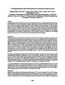
Figure 1. Cross-linked histograms for five U.S. census data attributes. The rectangular boxes show that only the Persons attribute has been restricted.

shaded bars against the backdrop of the histograms for the entire data set. This enables the analyst to visualize correlations and outliers in the data. For example, Figure 1 clearly shows that census blocks with many persons tend to span a wide area. Despite the obvious benefit of visual data exploration, most work in the database literature has not focused on meeting its requirements. Most visualization systems import a working set of data from a database, and include this active-dataset in every visualization. In our research, we have used a visualization tool, Visage [27, 9, 8, 7, 33], which allows users to update the active-dataset dynamically using drag and drop operations.1 Visage also maintains multiple active-datasets as-

1 Introduction Decision support systems often provide tools to visualize the data being analyzed. Rather than stare at tables of numbers, analysts can explore the features in the data by manipulating and viewing bar graphs, scatter plots, and other visual representations of the data. Figure 1, for example, shows a cross-linked histogram representation for five attributes of the U.S. census data. Users can subselect ranges of the data by manipulating the rectangles, called sliders, for each attribute. The five marginal 1-D histograms for the selected multidimensional range appear as darkly

1 Although we used Visage for concreteness (and it provided many attractive features), the results in this paper are not tied to a particular choice of visualization tool [6].

1

A1

sociated with different visualizations, so they can be compared or combined. For instance, outliers can be dragged out of a visualization to eliminate them from an activedataset, or clusters from two different visualizations can be dragged into an empty active-dataset to perform a union. Visual data exploration is an iterative process, where the results of one query suggest new queries or operations. The tasks of dataset definition, cleaning, and visualization design and interaction are interleaved arbitrarily. Rapid feedback is essential to exploration. Inherent human time scales for perception generate query response time constraints. Returning to the crosslinked histograms example, moving a slider continuously with the mouse changes one attribute’s range restriction as each pixel boundary is crossed, and the histograms for all other attributes must be updated (called dynamic queries [1]). If the updates take longer than 100ms, perceptual/motor coordination degrades very rapidly; with 200ms feedback a mouse is already very hard to use. In general, a visual data exploration system must translate a mouse move into a query, compute from the active-dataset a new value for all visualized parameters, and display them, all within 100ms or less. These stringent response times dictate that the activedataset size is limited to fit in main memory. Moreover, the desired query response times will not be met without indexes and/or precomputed totals on the active-dataset, and these too must fit in memory. Finally, we anticipate that a single dynamic query will need to continuously update up to a half dozen summaries. This leads to the following two requirements for any index or summary table computed for an active-dataset.

A2

A2 A3 A4

A3 A4 A4

A3 A4 A4

A5 A1

A3 A4 A4

A4 A5

..

A1

Figure 2. A kd-tree on d = 5 dimensions. N = 219 (≈ half a million), d = 5, and m = 28 , the datacube is over 28·5 · 19/(219 · 5 · 8) > 219 times larger than the active-dataset! Recent techniques for sparse or partially materialized data cubes [18, 26, 17] can dramatically reduce the required space, but at a significant cost in answer speed (see the discussion in Section 2). On the other hand, a data structure such as a kd-tree [5] (Figure 2), which satisfies the size requirement, fails to satisfy the time requirement. To gain intuition on why this is the case, consider a kd-tree that uses the attribute order A1 , A2 , . . . , Ad for partitioning on its d attributes, and a count query with an equality predicate on attribute Ad . Answering this query requires visiting all kd-tree nodes down to level Ad−1 , tracing a path from each such node for one level, then visiting all kd-tree nodes in the top d − 1 levels of those subtrees, and so on — a total of Θ(N 1−1/d ) nodes. RAD-trees. In this paper, we present a novel annotated index structure, called a RAD-tree, which meets both the time and size requirements, for significantly larger data sets than all previous approaches. RAD-trees are a novel extension of AD-trees [24], an index structure from the machine learning literature. RAD-trees overcome the query performance bottlenecks of AD-trees, by replacing each high-fanout node in the AD-tree by a range-based mini-tree, and performing other important optimizations. Moreover, RAD-trees significantly outperform kd-trees, by avoiding sifting and aggregating over attributes not in the query predicate, and performing other optimizations. In a nutshell, RAD-trees trade-off space for time, incurring a somewhat larger space overhead in order to significantly improve query times; we believe this is a desirable trade-off given the stringent response time requirements of visual data exploration.

• Time requirement: Using the indexes and summary tables, up to a half dozen multidimensional equality queries, range queries, and histogram queries on the active-dataset can be answered in 1 and A1 < 9 and A3 = 4 and A5 > 15 and A5 < 50 and A8 < 5

(b) Range query

Outline. The rest of the paper is organized as follows. In Section 2, we discuss previous work on index structures and summary tables. In Section 3, we present RAD-trees. In Section 4, we discuss our index performance visualization tool. In Section 5, we present extensions to RAD-trees for other types of queries and uses of RAD-trees in machine learning and other contexts. In Section 6, we report on experiments with census data and synthetic data. Conclusions are provided in Section 7.

select A2, count(*) from active-dataset where A4 > 9 and A7 < 20 group by A2

(c) Histogram query Figure 3. Example count query types. with the number of records in its subtree. By descending the tree, eventually nodes will be reached where either all the associated data will satisfy the query, or none of it will. The answer is then (1) all the records associated with the satisfying nodes, or (2) the sum of the counts stored at the satisfying nodes. Histogram queries are answered by computing separate totals for each value of the grouping dimension (A2 in Figure 3c).

2 Preliminaries and Related Work There are many existing tools and techniques for visualizing large tables of multidimensional numerical data (e.g., [30, 21, 3, 20, 22, 25, 23, 4, 31, 28, 34, 11, 29]). Ahlberg et al [1] introduced the use of dynamic queries, in which displayed plots and summaries are updated continuously with the movement of the mouse [2, 15, 12, 7]. Supporting these dynamic queries requires carefully designed index structures or summary tables that meet the time and space requirements outlined in Section 1. In this section, we discuss related work in index structures and summary tables, showing that these previous approaches fail to meet these requirements.

Summary tables. Multidimensional summary tables such as data cubes only address the second problem, by providing precomputed counts for various equality queries. Range count queries are answered by summing up the equality counts over the ranges. Histogram queries are answered by reporting the precomputed counts for each value of the grouping dimension. In the remainder of this section, we present further details on the salient multidimensional summary totals and indexes in the literature for answering equality, range, and histogram queries: data cubes, kd-trees, and AD-trees. We consider an active-dataset of N rows and d attributes. For notational simplicity, we assume in this section that each attribute has arity m, so that the active-dataset size is N · d · log m bits, although the arguments readily extend to sets of attributes with differing aritys.

Queries. For concreteness, we will focus on three types of multidimensional queries: (1) equality queries: count or selection queries with equality predicates on some or all of the attributes; (2) range queries: count or selection queries with at least one inequality predicate; and (3) histogram queries: count queries with equality or inequality predicates, grouped on a dimension (for use in cross-linked histograms). Examples are depicted in Figure 3, for count queries. In this paper, we use “attribute” and “dimension” interchangeably. We make the common assumption that each attribute is from a finite, discrete, ordered domain.3

2.1 Data cubes A data cube [16] stores the answers to all possible equality count queries over a set of (dimension) attributes. Thus answering equality count queries involves simply looking up the answer. However, as highlighted in Section 1, the fully materialized datacube has (m + 1)d entries, any of which may need to hold a count of up to log N bits. This is typically many orders of magnitude larger than the activedataset (e.g., nearly 6 orders of magnitude in the example in Section 1), and hence does not meet our size requirement for visual data exploration. There has been considerable work on reducing the size of data cubes or improving their query or update performance (e.g., [18, 26, 17, 19, 14, 32]). Work on sparse or partially materialized data cubes [18, 26, 17, 32] trades off decreases in size for increases in query times. Query times

Index structures. Multidimensional index structures [13] such as kd-trees, AD-trees, and our new RAD-trees address the problems of (1) finding the data records that satisfy a multidimensional range, and (2) finding the count of such records. The tree root is associated with the entire dataset, and child nodes are associated with subsets of the parent’s data. To facilitate count queries, each node is annotated 3 For categorical attributes, the ordering is often meaningless. For noncategorical attributes, the discrete domain often arises from a discretization of a more continuous domain into a fixed number of equi-width buckets (e.g., as is done in the U.S. census database). Although, for simplicity, we will view this discretization as fixed, Visage in fact discretizes on the fly when building an index: the range of each selected attribute is bucketized into 256 equi-width buckets for histogramming purposes.

3

2.3 AD-trees

increase because (1) the components of a partially materialized cube must be assembled at query time, and (2) we need a means to locate the desired counts in the sparse representation. Moreover, data cubes are not well suited for range queries (unless the entire range is desired), because we need to sum up individual cube values to compute the range count, and this can be up to Θ(N ) entries!

AD-trees were introduced by Moore and Lee [24], to enable fast computation of contingency tables. A pivot table represented in relational form is called a contingency table in the machine learning literature. Contingency tables are used to build the probability tables for Bayes nets and evaluate conjunctive rules in rule learning algorithms [24]. Fixing values in a contingency table is equivalent to slicing a data cube. AD-trees were designed to support only equality count queries. Moore and Lee provide a brief qualitative comparison of AD-trees with kd-trees and R-trees, but no quantitative or experimental comparison. AD-trees improve upon the equality count query performance of kd-trees by adding a sufficient number of branches to the tree so that an equality count query on any combination of attributes can be answered without sifting through nodes for attributes not in the query. Also, instead of binary splitting at a node, it does m-way splitting. Moreover, it adds extra nodes containing counts of the number of records in its subtree. In further detail, there are two types of nodes in AD-trees: count-nodes and vary-nodes. The parent of a count-node is a vary-node, and vice versa. A count-node for attribute Ai has d − i children, each of which is associated with the same data as the parent and with one attribute. Therefore the space complexity is much higher than that of a kd-tree. A vary-node has m children, where m is the number of values that the parent attribute takes. Conceptually, the children partition the node’s data by the values of the parent attribute. The height of the tree is 2d and the total size is O(md (log N + log m)) bits [24]. Although this worst case size bound is almost as bad as data cubes, the size is reduced dramatically for skewed distributions because of the following AD-tree optimizations: (1) space is not allocated for counts of zero, (2) space is not allocated for counts that can be deduced by other counts, and (3) the tree is not expanded fully near its leaves. In further detail, the main space saving optimization is to eliminate the largest subtree of count-nodes, because counts in that subtree can be found from the remaining information. Thus each vary-node has one count-node child that has been eliminated. This child is called the nulled node. This optimization has a huge impact, and AD-trees are not too much larger than kd-trees for the data sets we studied (see Section 6). Additional space savings are obtained by truncating the tree at each node with fewer than a fixed threshold number of records (Moore and Lee used a threshold of 16). Instead, the truncated node stores pointers to the records. See [24] for further details. The main problem with AD-trees is that they are not well-suited for range queries. We will show in Section 6 that range queries on AD-trees are up to 3 orders of magnitude slower than equality queries, because the search/aggregate must branch at almost every vary-node, rather than only in the case where the equality predicate selects the vary-node’s nulled node.

Alternatively, for quick answers to range queries, we could use a partial-sums cube [19], where the entry for the jth value of an attribute is the count up through the jth value. However, the cube is no longer sparse: the space requirements for the prefix-sum cube are as bad as for the fully-materialized cube! Ho et al. [19] present techniques for reducing the space somewhat, at a cost of increasing the query time. Finally, we could build an index on top of the sparse cube that supported fast range queries. This just reduces the problem to designing a good multidimensional index (the topic of this paper): Nothing was gained by using a datacube! In summary, the data cube and its variants are very far from meeting the requirements for visual data exploration, and hence we dismiss them from further consideration in the rest of this paper.

2.2 kd-trees In a kd-tree [5] (Figure 2), the children of a node partition the parent’s data into two subsets using a cutoff value of one of the attributes. The goal is to obtain nearly equal sized partitions, so that the height of the tree will be approximately log N . The attribute used to partition a node can be deterministic or adaptive. In the former case, the attributes are ordered and the root partitions the first attribute. Other nodes use the next attribute after the one its parent uses, or the first attribute if the parent uses the last attribute. A kd-tree contains O(N ) nodes; typically each node contains a split dimension, a split value, and left and right subtree pointers, for a total size of O(N · (log d + log m + log N )) bits. In order to take advantage of any gaps in the data ranges, the bounding hypercube for each node is sometimes stored. If the active-dataset records are stored inside the kdtree, the space bound increases by at most a constant factor. Thus kd-trees satisfy the size requirement. Equality count queries take O(N 1−1/d ) time. In the best case of a point query (equality predicates on all dimensions), the query takes only O(log N ) time. However, the common case of a count equality predicate on a single attribute is Θ(N 1−1/d ) time regardless of the attribute. Range queries and histogram queries are even worse, taking O(N ) time. As discussed in Section 1, the problem is that multiple paths must be examined. Thus in all cases, query times for common queries are asymptotically slow, and as our experiments in Section 6 demonstrate, query times on real datasets can be too slow to meet the time requirement. 4

child of the root, and then visit an A3 child of that A1 child. Whereas kd-trees incur large overheads because they must sift through a large number of subtrees for each attribute not in the predicate, these paths ensure that RAD-trees avoid such overheads.

ROOT

A1

A2

... A2

... A3

A3

A3

... A2

... A3

A3

A3

A3

A3

Mini-trees. In further detail, the RAD-tree alternates varynodes and mini-trees of count-nodes. A RAD-tree on two attributes A1 and A2 is shown in Figure 5. (The subtree rooted at A1 = [4..6], which is omitted from the figure, is similar to its sibling subtrees.) A1 is from the domain [1..9] and A2 is from the domain [1..3]. The vary-nodes are shown as ovals; they indicate which attribute is being varied in their children count-nodes. The count-nodes are shown as rectangles, with the notation “#[x,y]” indicating that the node holds a count of the number of records that have both A1 = x and A2 = y. For example, the root count-node stores the total number of records (“*” is a wildcard), and the lower rightmost count-node stores the number of records with A1 ∈ [7..9] and A2 = 3. The larger the arity of the attribute, the more levels in the mini-tree. In this figure, we use a two-level mini-tree for A1 and a one-level mini-tree for A2. The use of multi-level mini-trees is one of the key improvements of RAD-trees over AD-trees. In a 2-level minitree √ first level represents √ over attribute j with arity m, the m non-overlapping subranges of m values each.4 Each √ of these nodes in the first level of the mini-tree has m count-node children (one for each of the values in the subrange) and d − j vary-node children (one for each of the remaining attributes). Each of the count-nodes in the second level have d − j vary-node children. See Figure 5. In general, in an i-level mini-tree for an attribute (with arity m), the top level represents m1/i non-overlapping subranges of m1−1/i values each, and each of these nodes has m1/i count-node children representing subranges of m1−2/i values each, and so on. Only the nodes at the (i − 1)th and ith levels have vary-node children, with each having d − j such children. Mini-trees mitigate a problem with AD-trees, namely that range queries and even many equality queries require performing subqueries over all individual data values in a range. The cost for this is proportional to the fanout of the associated vary-node. By aggregating on subranges, we reduce this fanout, at a cost of additional levels. For example, for an attribute with arity m, an AD-tree accumulates the counts from m siblings, while a RAD-tree with a 2-level √ mini-tree accumulates the counts from m nodes at the first level and then recurses on one or two of these nodes,√depending on the query ranges, each of which has fanout m. Thus the speed up of RAD-trees √ √over AD-trees are roughly proportional to m/(2 m) = m/2. In constructing the RAD-tree, we determine the desirable number of levels for the given m, based on a lower bound on the fanout at each level. In the datasets we studied, the best choice mini-trees

A3

Figure 4. High-level view of a 3 attribute RADtree

2.4 Summary of Prior Work In summary, none of the previous work satisfies both the time and size requirements for visual data exploration. Thus a new structure is needed. We propose using a novel annotated index that obtains nearly the best of data cubes, kdtrees, and AD-trees, without their unacceptable costs.

3 RAD-trees In this section, we introduce our novel data structure, called the RAD-tree. RAD-trees address the problems with previous approaches as follows. • Precomputing all summary totals takes too much space: Instead, we use a tree-like data structure to implicitly represent the totals. • kd-trees must sift through a large number of subtrees for each attribute not specified by the query: Instead, we implicitly represent all possible combinations of queried attributes, and hence avoid this sifting through. • AD-trees frequently traverse and sum up subtrees for all the individual values in a range: Instead, we preaggregate sets of ranges, and replace each large fanout vary-node with a range-based mini-tree (discussed below). After describing the basic RAD-tree design in this section, we will present a number of optimizations in Section 4.

3.1 Basic Design At a high level, a RAD-tree has the same basic structure as the AD-tree. There are count-nodes and vary-nodes. To accommodate an arbitrary subset of the attributes in a query predicate, RAD-trees have subtrees for all the combinations. Figure 4 depicts the high-level view of a RAD-tree on three attributes A1, A2, and A3. Each subtree labeled A1 (A2, A3) in the figure fans out to individual values for A1 (A2, A3, respectively). As can be seen from the figure, for any of the 23 combinations of attributes appearing in a predicate, there are paths through the RAD-tree (starting at the root but not necessarily ending at a leaf) that pass through precisely this combination. For example, paths for precisely attributes 1 and 3 start from the root, visit the A1

4 For simplicity, we assume all such quantities are integers; although the implemented code handles the general scenario.

5

ROOT #[*,*]

vary A1

A1=[4..6] #[4..6,*]

A1=[1..3] #[1..3,*]

A1=1 #[1,*]

A1=2 null

vary A2 A2=1 #[1,1]

A2=2 #[1,2]

A1=3 #[3,*]

A2=1 null

A2=2 #[3,2]

A1=7 #[7,*]

vary A2 A2=1 null

A2=3 A2=2 #[1..3,2] #[1..3,3]

A2=3 #[3,3]

A2=1 null

A1=[7..9] #[7..9,*]

..

vary A2 A2=3 null

vary A2

A1=8 #[8,*]

A2=2 #[7,2]

A2=3 null

A2=1 #[8,1]

A2=2 null

A2=3 #[*,3]

vary A2 A2=1 #[7..9,1]

vary A2

vary A2 A2=1 #[7,1]

A1=9 null

A2=2 #[*,2]

A2=2 null

A2=3 #[7..9,3]

A2=3 #[8,3]

Figure 5. RAD-tree on two attributes, using a two-level mini-tree for A1 and a one-level mini-tree for A2.

tended to have at most five levels. Saving space. We dramatically reduce the space needed by eliminating each count-node that (1) is a leaf of its minitree, and (2) has the largest count among its immediate siblings (ties broken arbitrarily). In Figure 5, for example, the middle child subtree of the A1 = [1..3] countnode is removed (indicated by null) because #[2,*] is greater than #[1,*] and #[3,*]. In the typical case of skewed data, eliminating the largest subtrees reduces the space significantly. Our construction of mini-trees ensures that queries that would normally be answered by following paths into the removed subtrees can be answered by combining counts elsewhere in the tree (just as in the simpler AD-trees). Additional space savings are obtained by truncating the tree at each node with fewer than a fixed threshold number of records (e.g., 16), as in AD-trees.

The second subcase to consider is when the nulled node is a leaf in a multi-level mini-tree. This subcase is conceptually the same as the previous subcase, but the explanation is slightly different. We first compute the count c for the original query where the predicate on attribute i is replaced by the predicate on i in the parent of the nulled node. Then for each of the siblings of the nulled node, we compute the counts using the sibling subtrees (where the predicate on i is replaced by the predicate on i for the sibling) and subtract these from c. Example 2: Consider the query select count(*) from active-dataset where A1=2 and A2=2. The path through the RAD-tree for this query encounters the nulled node for A1 = 2. This eliminated node is in a 2-level minitree. We first compute c = #[1..3,2] and then subtract #[1,2] and #[3,2] to obtain the desired count, i.e., #[2,2] = #[1..3,2] - #[1,2] - #[3,2].

3.2 Queries Query results are built by recursively descending the RAD-tree. Figure 6 presents pseudocode for the procedures invoked at each step of the recursion. The only difficult case is when the query range overlaps one or more nulled nodes, discussed next. To compute a count from a nulled node of some attribute i, there are two subcases to consider. If the nulled node is in a 1-level mini-tree, then we first compute the count c for the same query ignoring the predicate on this attribute. Then for each of the siblings of the nulled node (recall that there is only one nulled node per set of siblings), we compute the counts using the sibling subtrees and subtract these from c to get the desired exact count. Example 1: Consider the query select count(*) from active-dataset where A1=1 and A2=3. The path through the RAD-tree for this query encounters a nulled node (the third leaf from the left in the figure). This eliminated node is in a 1-level mini-tree. We first compute c = #[1,*] and then subtract #[1,1] and #[1,2] to obtain the desired count, i.e., #[1,3] = #[1,*] - #[1,1] - #[1,2].

4 Visualization-Driven Index Optimizations Understanding the behavior of multidimensional, dataadaptive indexes is quite challenging, when trying to explain and tune their space usage and query performance. In this section, we describe a simple tool we created for visualizing data-dependent indexes and their use in answering aggregate queries. Although there are many available visualization tools [6], to our knowledge, previous work on database indexes has not focused on the use of such tools for visualizing performance bottlenecks, and hence has not studied how much performance improvements they can provide. This section quantifies (albeit somewhat informally) the performance improvements we obtained, showing how our tool guided us to optimizations that sped up RAD-tree query times by a factor of 6. Moreover, the examples depicted in this section provide insights into what makes RAD-trees an effective multidimensional index. 6

Figure 7. Visited nodes: AD-tree on the left, RAD-tree on the right

4.1 Visualizing Data-Dependent Indexes

tree (left) with the performance using a RAD-tree(right). The RAD-tree uses two-level mini-trees. From the figure, it is apparent that answering the query on the AD-tree requires significantly more node visits and comparisons than answering the query on the RAD-tree (the AD-tree figure is much denser). Indeed, our experiments show that a random such query runs on average an order of magnitude slower using AD-trees compared to RAD-trees. A key aspect of the savings is the use of mini-trees to avoid visiting all the individual values in a range. This is confirmed by the absence of large fanout nodes in the RAD-tree plot compared to the AD-tree plot. The extra levels of the mini-trees are confirmed by the extra levels in the RAD-tree plot.

Data-dependent indexes such as AD-trees and RADtrees dramatically adapt their shape to the underlying multidimensional data. Moreover, due to their various space saving techniques (such as truncating sparse portions of the tree, and nulling out the largest subtree at a node), the resulting shape is not easily pictured without further visual aids. Because it is difficult to picture the shape of an index for a given active-dataset, much less the nodes visited in answering a query, it is often challenging to grasp or predict why particular queries are fast and others are slow, to find bugs in implementations, and to assess which optimizations for the index are likely to have maximal benefit. To help with these issues, we created a new tool that graphically displays which parts of the index are visited during queries. The tool collects a trace file for the nodes visited during a query, which is fed into a visualization front end for display as a weighted and colored tree. A user selects up to three features of the tree to highlight using the color, sizes, and labels of nodes, and up to three features to highlight using the color, sizes, and labels of links. An example output is shown in Figure 7. In this example, the active-dataset is 50,000 records selected from a U.S. census dataset, projected to five attributes of arity 128 (i.e., N = 50, 000, d = 5, and m = 128). A range count query is chosen by randomly selecting the limits of the range for each attribute, where the lower limit is chosen from the bottom 10% of the range and the upper limit is chosen from the top 10% of the range (called a Big Range query in Section 6). The same query is used for the figure on the left and on the right. For this particular visualization, we have selected that the width of both the link and the node indicate the number of comparisons made in visiting the node.5 The figure contrasts the performance of the query using an AD-

4.2 Optimizing RAD-trees When we were developing our new index, we used our index-visualization tool in an iterative process in which we would uncover a performance bottleneck, try out possible optimizations to fix it, select the best fix, and move on to the next bottleneck. We parameterized the RAD-tree code so that optimizations could be turned on and off at will. It is often quite difficult to anticipate how various index optimizations will interact: Do their individual effects complement one another or cancel one another out? By comparing side-by-side a plot with optimization 1, a plot with optimization 2, and a plot with both 1 and 2, we can visualize this interaction effect. We now describe several optimizations to RAD-trees suggested to us by the index visualization. Leaf list indexes. We discovered that in an early version of our index, most of the query time was being spent stepping through the leaf lists. Each leaf list contained a collection of record pointers; the records were fetched to see which satisfied the query predicate. (Recall that we store pointers, not the records themselves, because in the worst case, a single record can appear 2d times in the tree.) Consider

5 In this paper, we have rendered all figures in black and white, for ease of printing. Of course, the tool is more effective when its color features are used.

7

-------------------------------------------// In this pseudocode, Q is the query, n is // the (index of the) query attribute under // consideration, and L(Qn) [U(Qn)] is the // lower [upper] bound on the attribute’s range. // The overall count is computing by invoking: count-node-count(, Q, 1) Begin count-node-count(Ci, Q, n) unconstrained_count = vary-node-count( next-vary-sibling(parent(Ci)), Q, n+1) count = SUM over m = L(Qn) to U(Qn) If child(Ci, m) is a count node count-node-count(child(Ci, m), Q, n+1) Else vary-node-count(child(Ci, m), Q, n+1) neg-count = SUM over m = 1 to L(Qn)-1 and m = U(Qn)+1 to arity(Qn) If child(Ci, m) is a count node count-node-count(child(Ci, m), Q, n+1) Else vary-node-count(child(Ci, m), Q, n+1)

Figure 8. Motivation for leaf list indexes number of slow comparisons can be observed by comparing Figure 8 with the right plot of Figure 7. The only difference between these two plots is that the latter uses leaf list indexes. Although the same index nodes were visited (as expected), the number of comparisons is dramatically reduced in the latter figure (note the Figure 8 scale ranges from 0 to 2000, while the Figure 7 scale ranges only from 0 to 350). Indeed, our experiments showed that this optimization sped up queries by a factor of 4 on average. Early pruning on zeros. A second optimization whose effectiveness was evident from the index visualization plots was to perform early pruning on the subquery generated to calculate the count when encountering a nulled node. The plots showed6 that almost all of the subqueries to count the matching records in a subtree return 0. Recall from Section 3.2 that computing the count for a nulled node involves first computing the count for the same query ignoring the nulled attribute and then subtracting counts computed from sibling subtrees. If the first query returns 0, then the sibling subtree counts can be skipped (they too will be 0), because we know the count for the nulled node is 0. It was not clear a priori whether this straightforward optimization would have a sufficiently large performance impact to warrant its inclusion into the RAD-tree algorithm. However, the visualization plots showed (and the experiments confirmed) that the optimization pays off big for equality queries (a factor of 3 speedup) but has only a modest improvement for range queries (10%–20%). This is reasonable in view of the fact that hitting a nulled node is by far the worst case for an equality query, but makes things only slightly worse for a range query, which has to search multiple sibling subtrees in any case. A possible optimization that failed. We also tried keeping the minimum and maximum value for each attribute across all the records for a leaf node. Then two special cases return quickly. If the query range is disjoint from one of the

If Ci is a leaf return the count of leaf-list records matching Q Else If Q[n] is unconstrained // no predicate on this attribute return unconstrained_count Else if Q[n] does not include the nulled node for Ci, return count Else return unconstrained_count - neg-count EndIf End Begin vary-node-count(Vi, Q, n) return SUM over m = L(Qn) to U(Qn) count-node-count(child(Vi, m), Q, n) End --------------------------------------------

Figure 6. Pseudocode for RAD-tree queries. Figure 8, which shows the visited nodes and the number of leaf list fetches (denoted slow comparisons) for the same dataset and query as before. As depicted in the figure, the number of slow comparisons was often in the hundreds per leaf for this early version of our index. Yet often most of the records fetched failed to satisfy the predicate. To mitigate this effect, we added mini-indexes for each leaf list. Specifically, when constructing the index, we sort each leaf list by the first relevant attribute A and store the pointers in an array L. For quick lookups, we create and store an array I of m entries, where I[j] stores the first position in L for a record with value j for attribute A. This simple mini-index enables us to answer a query by jumping immediately to the start of the predicate range and fetch only those records up to the end of the range; these are the records that need further checking. If there are no more attributes to check, the process is even simpler: the difference between the start and end pointers is the desired count. The effectiveness of this optimization in reducing the

6 Because of page limitations, many of our plots are omitted here, but can be found in the full technical report [10].

8

6 Performance Study

attribute ranges, the count must be zero. If the query range is contained in all of the attribute ranges, the count includes all records. This produced a speedup of 30% by itself, but worsened the speedup in combination with the other techniques. Most of the leaf nodes have no more than one attribute to check, in which case sorting the leaf lists has all the advantages of range checking, plus if the special cases are not met, the search is still reduced to only those records that match on the first attribute. Thus we dismissed this possible optimization.

The bulk of this section presents experimental results on U.S. census data. We compare the effectiveness of RADtrees, kd-trees, and AD-trees for arbitrary equality queries, range queries, and histogram queries, varying the dataset size, the number of attributes, the number of predicate attributes, and attribute arity. We also report on construction times and index sizes. Finally, in order to explore the effect of data skew, we present results for synthetic data generated according to various zipf distributions.

5 Extensions 6.1 Experimental setup In this section, we show that a RAD-tree provides an effective annotated index for providing exact answers to aggregate queries over multidimensional data (up to 5 dimensions) in milliseconds, for a variety of scenarios beyond visual data exploration, given simple extensions to the basic RAD-tree design. Although we have focused on count queries in the text, RAD-trees can be used for selection queries by returning the records instead of just the counts. This could be used to generate dynamic scatter plots. In order to make this work, we need to store the record pointers (record ids) for the records associated with RAD-tree leaves. To avoid reporting duplicate tuples, we mark a tuple the first time we fetch it (alternatively, we can build a hash table). With the same enhancement, RAD-trees can readily compute and report other aggregates such as sums and averages. In fact, arbitrary aggregate expressions such as sum(A1 + 4*A2) can be computed because we can quickly retrieve all the records satisfying the query predicate. We can store and process queries on multiple measure attributes. We can also generalize the histogram query to more general group-by queries, or pivot tables. We can produce fast, approximate answers to queries by extracting a (possibly stratified) sample of the data for our active-dataset. It is easy to account for the varying scale factors arising in stratified sampling within the same activedataset, and report error guarantees. Similarly, we can quickly provide and visualize early results for multidimensional selection queries on data sets too large to fit in main memory, as follows. We use the RADtree on a memory-resident subset of the data to return, in a fraction of a second, records that satisfy the selection. Then, while the user is exploring these records, the DBMS can compute the complete answer from the full database. This approach is effective if the memory-resident subset contains records satisfying the selection; in certain cases such as large multi-way joins, the subset may not have the needed joining tuples. Thus RAD-trees can be used for a variety of data analysis scenarios. For example, as discussed in Section 2, a pivot table represented in relational form is called a contingency table in the machine learning literature. Contingency tables are used to build the probability tables for Bayes nets and evaluating conjunctive rules in rule learning algorithms.

We ran an extensive set of experiments comparing RADtrees, kd-trees, and AD-trees. The experiments were run on a 1.2 GHz Pentium 4 laptop with 1 GB of main memory, running Windows 2000. We implemented the code to construct and query the kd-trees and RAD-trees; for the ADtrees, we obtained the code from Andrew Moore [24]. Data set and queries. In our base configuration, we have an active-dataset of 500,000 records from the U.S. census database, with 5 attributes per record. Each attribute has been discretized into 256 equal width bins (so that m = 256). We compare the three indexes on four types of count queries: • Equality query (Figure 3(a)): Each query is chosen by selecting an attribute A uniformly at random and an attribute value v uniformly at random from [0..255], and posing the query select count(*) from active-dataset where A=v. • Range query (Figure 3(b)): Each query is chosen by selecting attribute value Li uniformly at random from [0..255] and attribute value U i uniformly at random from [Li..255] for each attribute Ai, and posing the query: select count(*) from active-dataset where A1 = L1 and A2 = L2 and A3 = L3 and A4 = L4 and A5 = L5.

• Big Range query: same as range query, except that each Li is restricted to be in the bottom 10% of the value range (i.e., [0..25]) and each U i is restricted to be in the top 10% of the value range (i.e., [230..255]). • Histogram query (Figure 3(c)): same as big range query, except that we repeat for each attribute Ai, adding a group by Ai clause to the query. For each type of query, we repeat the experiment for 10 seconds or 1000 queries, whichever takes longer, and report the average response time. In addition, we ran an extensive set of experiments starting from the base configuration but varying the size of the 9

kd-trees AD-trees RAD-trees

Equality 3.755 0.012 0.012

Range 0.823 6.609 1.162

Big Range 15.913 12.158 0.968

Histogram 77.802 22.265 6.540

Figure 10. Response time in microsecs for big range queries, varying the number of records.

Figure 9. Average single query response times in millisecs for kd-trees, AD-trees, and RAD-trees on the U.S. census data set. Top: A table of response times. Bottom: The data plotted using a log scale.

better on big range queries because they are well-suited to aggregating over ranges. Both RAD-trees and AD-trees improve dramatically on histogram queries, compared to kdtrees. In summary, the results in Figure 9 show that • RAD-trees are faster than kd-trees for three of the query types, including over 300 times faster on equality queries, over 16 times faster on big range queries, and over 16 times faster on histogram queries.

dataset, the number of attributes, the attribute arity, or the number of attributes in the predicate7.

6.2 Query Time Comparisons • RAD-trees match the performance of AD-trees for equality queries, and are over 6 times faster on range queries, over 13 times faster on big range queries, and 3.5 times faster on histogram queries.

Figure 9 shows the response times for the queries in the default configuration. Because RAD-trees can be a order of magnitude or more faster, the response times are plotted on a log scale. kd-trees perform poorly on histogram queries. This poor performance is to be expected, given that 5 histograms must be computed and each involves aggregating a collection of histogram buckets over a large number of tree nodes. Big ranges also suffer from aggregating over a large number of tree nodes, although not as badly as histograms because there is only a single total to accumulate. Equality queries suffer somewhat from aggregating over O(N 1−1/d ) nodes. On the other hand, range queries do quite well on kdtrees, because each attribute range selects an expected one third of the range, so with 5 attributes, we expect only about 1/35 ≈ .4% of the nodes to satisfy the query predicate. RAD-trees and AD-trees are a dramatic improvement over kd-trees for equality queries, because they avoid sifting through and aggregating over individual nodes for attributes not in the query. AD-trees perform poorly on range and big range queries, because they must aggregate over individual values for the attributes in the predicates. In fact, AD-trees can not take much advantage of the high selectivity of range queries because each null bucket encountered converts a 1/3 range into a recursive call that aggregates over the entire range of another attribute. On the other hand, RAD-trees perform nearly as well on range queries and dramatically

• Thus considering either big range or histogram queries, kd-trees fail to meet our goal of supporting up to a half dozen simultaneous queries in well under 100 millisecs. Likewise, AD-trees fails to meet our goal for histogram queries. RAD-trees, on the other hand, meet our goal for all query types, and in fact, can readily support a dozen simultaneous queries. Varying dataset size, number of attributes, number of predicate attributes, and attribute arity. We ran an extensive set of experiments varying these four parameters from our base configuration [10]. Figure 10 shows that the advantage of RAD-trees for big range queries only increases with increasing active-dataset size. Other query types were similar. Our results also show that the advantage of RAD-trees only increases with increasing (albeit only modest) dimensionality. In addition, our results show that the gap between RAD-trees and kd-trees increases dramatically as the number of predicate attributes decreases (the total number of attributes is unchanged), because each attribute that is not a predicate attribute forces additional kd-tree sifting. We also studied the effect of attribute arity on the performance, and found no surprises: for all query types, the response time increased dramatically with increases in the arity, similarly for all indexes.

7 That is, whereas the base configuration range query has constraints on all 5 attributes, we will consider range queries with constraints on only 1–4 attributes (out of the 5).

10

Figure 11. Left, index size (in MBs) vs. number of records. Center, index size (in MBs) vs. attribute arity, shown on a log scale. Right, build time (in seconds) vs. number of records.

6.3 Tree sizes and construction times Next, we compare the size of the indexes, under various configurations. The left and center plots in Figure 11 show how the index sizes vary with the number of records and the attribute arity, respectively, in the active-dataset. We also studied how the the index sizes vary with the number of attributes [10]. These results show that the dramatic improvement in query times for RAD-trees comes at a cost of a nontrivial increase in space: In almost all cases, RADtrees use the most space. For the base configuration, RADtrees use 3.8 times the space of kd-trees and 2.6 times the space of AD-trees. RAD-trees appear to scale sublinearly with data size, but superlinearly with arity and number of attributes. We do not view the arity scaling as a serious drawback because arity 28 is a good choice for the visualizations in Visage. On the other hand, the superlinear scaling in the number of attributes implies that RAD-trees are not well suited to visualizing an active-dataset of more than five dimensions at a time.8 In the largest configuration, the RAD-tree used only 135MBs out of the available 1 GB of memory. Next, we compare the construction times for the three indexes, under various configurations. The plot on the right of Figure 11 shows the construction times as a function of the number of records in the active-dataset. All indexes appear to scale sublinearly with data size. kd-trees are slightly faster to build, but all indexes are built in under 30 seconds.

Figure 12. Query response times in millisecs for kd-trees, AD-trees, and RAD-trees for zipf=1.2 data (log scale).

zipf data. Here we report only on one such set of experiments (further results are in [10]). For this set, we used a summarized reporting of the equality, range, big range, and histogram query results: Instead of fixing the number of attributes in a query predicate, each query (in the 1000 queries in an experiment for a given query type) selects at random whether the query predicate was on 1, 2, 3, 4, or 5 attributes. Figure 12 shows the response times for queries with moderate skew (zipf=1.2). In summary, these results show that: • RAD-trees are a factor of 5.6, 1.2, 1.8, and 3.8 faster than kd-trees on equality, range, big range, and histogram queries, respectively.

6.4 Varying the data skew We conclude this section by examining the effect of data skew. For these experiments, we use a synthetic activedataset of 2,000,000 records, each with five attributes, where the attribute values are generated independently according to a zipf distribution. We consider zipf parameters ranging from 0.7 to 2.0. The experimental setup is the same as in Section 6.1, except that we use zipf data instead of census data. We conducted a wide range of experiments on

• RAD-trees are considerably slower than AD-trees on equality queries (although still quite fast: 0.134 milliseconds) and a factor of 2.1, 7.0, and 5.4 faster than AD-trees on range, big range, and histogram queries, respectively. • AD-trees fails to meet our time goal for big range and histogram queries. kd-trees fails to meet our time goal for histogram queries. RAD-trees, on the other hand, easily meet our time goal for all query types.

8 Note that these five dimensions in the active-dataset can be extracted from a (full) data set with an arbitrary number of dimensions.

11

7 Conclusions Motivated by the demands of visual data exploration, we have introduced RAD-trees, an annotated index structure that in many cases improves query times by factors of 3– 300 over the best previous approaches for multidimensional data (up to 5 dimensions) of modest-to-high skew. Therefore, we recommend RAD-trees for delivering mouse-move speed response times to visual data exploration and analysis.

References [1] C. Ahlberg, C. Williamson, and B. Shneiderman. Dynamic queries for information exploration: An implementation and evaluation. In Proc. ACM Conf. Human Factors in Computer Systems CHI, pages 619–626, 1992.

Figure 13. Query response times in millisecs for (front-to-back) RAD-trees, kd-trees, and AD-trees, for zipf data of various skews (log scale).

[2] C. Ahlberg and E. Wistrand. IVEE: An environment for automatic creation of dynamic queries applications. In Proc. ACM Conf. Human Factors in Computer Systems CHI, 1995.

Figure 13 summarizes the results across various levels of skew (the zipf=1.2 case is repeated in the figure for comparison purposes). In all cases and for all three tree types, equality queries were plenty fast (at most 2.3 milliseconds), and hence this query type is omitted from the figure. (For such queries, AD-trees were the fastest, kd-trees were by far the slowest, and RAD-trees were in the middle.) When all attributes have low skew (zipf=0.7), RADtrees perform somewhat better than AD-trees (up to a factor of 2.5 faster) and on par with kd-trees (sometimes better, sometimes worse). This is expected because the space saving optimizations in RAD-trees (and in AD-trees) require at least modest skew to be effective. Thus neither are recommended for low skew data. Moreover, none of the tree types meet our time goal. However, most real-world data sets are skewed (e.g., the census data). When all attributes have modest skew (zipf=1.0)9, RAD-trees significantly outperform AD-trees (e.g., by a factor of 3.3 for histograms) and somewhat outperforms kd-trees (e.g., by a factor of 1.5 for histograms). As the skew increases, RAD-trees continue to be the fastest overall (e.g., a factor of 3.6–4.1 faster than kd-trees for zipf=1.5), until at very high skew (zipf=2.0), all techniques are quite fast. As before, these results are explained by the fact that RAD-trees avoids the overheads incurred by kd-trees in sifting through individual nodes for attributes not in the query, and the overheads incurred by both kd-trees and AD-trees in aggregating individual nodes that lie within range predicates. Note that the speed ups for RAD-trees are less dramatic than in our census data experiments. Using our index visualization tool, we have observed that RAD-trees advantageously exploit the correlations between attributes in the census data; these opportunities are missing in the synthetic data because all attributes are independent.

[3] A. Aiken, J. Chen, M. Stonebraker, and A. Woodruff. Tioga2: A direct manipulation database visualization environment. In ICDE, pages 208–217, 1996. [4] P. Au, M. Carey, S. Sewraz, Y. Guo, and S. M. Ruger. New paradigms in information visualization. In SIGIR, pages 307–309, 2000. [5] J. L. Bentley. Multidimensional divide and conquer. Communications of the ACM, 23(4):214–229, 1980. [6] S. K. Card, J. D. Mackinlay, and B. Shneiderman. Readings in Information Visualization–Using Vision to Think. Morgan Kaufman, 1999. [7] M. Derthick, J. Harrison, A. Moore, and S. F. Roth. Efficient multi-object dynamic query histograms. In Information Visualization, pages 84–91, 1999. [8] M. Derthick, J. Kolojejchick, and S. F. Roth. An interactive visual query environment for exploring data. In ACM Symposium on User Interface Software and Technology, pages 189–198, 1997. [9] M. Derthick, J. A. Kolojejchick, and S. F. Roth. An interactive visualization environment for data exploration. In KDD, pages 2–9, 1997. [10] M. A. Derthick and P. B. Gibbons. RAD-tree: A fast multidimensional index for visual data exploration. Technical report, Intel Research Pittsburgh, 2004. [11] P. R. Doshi, E. A. Rundensteiner, M. O. Ward, and D. Stroe. Prefetching for visual data exploration. In 8th Int’l Conf. on Database Systems for Advaced Applications (DASFAA), 2003. [12] K. P. Fishkin and M. C. Stone. Enhanced dynamic queries via movable filters. In ACM Conference on Human Factors in Computing Systems (CHI), pages 415–420, 1995. [13] V. Gaede and O. G¨unther. Multidimensional access methods. ACM Computing Surveys, 30(2):170–231, 1998. [14] S. Geffner, D. Agrawal, and A. El Abbadi. The dynamic data cube. Lecture Notes in Computer Science, 1777:237, 2000. Proc. EDBT’00.

9 This

is a commonly occurring skew, e.g., it is the skew in the distribution of words in text corpora.

12

[15] J. Goldstein and S. Roth. Using aggregation and dynamic queries for exploring large data sets. In Proc. ACM Conf. Human Factors in Computer Systems CHI, pages 23–29, 1994.

[33] J. Welling and M. Derthick. Visualization of large multidimensional datasets. In Virtual Observatories of the Future 2000, 2000.

[16] J. Gray, S. Chaudhuri, A. Bosworth, A. Layman, D. Reichart, M. Venkatrao, F. Pellow, and H. Pirahesh. Data cube: A relational aggregation operator generalizing group-by, cross-tab, and sub-totals. J. Data Mining and Knowledge Discovery, 1(1):29–53, 1997.

[34] J. Yang, M. O. Ward, and E. A. Rundensteiner. InterRing: An interactive tool for visually navigating and manipulating hierarchical structures. In InfoVis, 2002.

[17] H. Gupta, V. Harinarayan, A. Rajaraman, and J. D. Ullman. Index selection for OLAP. In ICDE, pages 208–219, 1997. [18] V. Harinarayan, A. Rajaraman, and J. D. Ullman. Implementing data cubes efficiently. In Sigmod, pages 205–216, 1996. [19] C.-T. Ho, R. Agrawal, N. Megiddo, and R. Srikant. Range queries in OLAP data cubes. In Sigmod, pages 73–88, 1997. [20] Y. Ioannidis. Dynamic information visualization. ACM SIGMOD Record, 25(4):16–20, 1996. [21] D. A. Keim and H. Kriegel. VisDB: Database exploration using multidimensional visualization. Computer Graphics and Applications, 1994. [22] M. Livny, R. Ramakrishnan, K. Beyer, G. Chen, D. Donjerkovic, S. Lawande, J. Myllymaki, and K. Wenger. DEVise: integrated querying and visual exploration of large datasets. In Sigmod, pages 301–312, 1997. [23] P. McCartney and K. J. Goldman. End-user visualization and manipulation of distributed aggregate data. Journal of Visual Languages and Computing, 10(3):193–213, 1999. [24] A. W. Moore and M. S. Lee. Cached sufficient statistics for efficient machine learning with large datasets. Journal of Artificial Intelligence Research, 8:67–91, 1998. [25] C. Olston, A. Woodruff, A. Aiken, M. Chu, V. Ercegovac, M. Lin, M. Spalding, and M. Stonebraker. DataSplash. In Sigmod, pages 550–552, 1998. [26] K. A. Ross and D. Srivastava. Fast computation of sparse datacubes. In Proc. 23rd Int. Conf. Very Large Data Bases (VLDB), pages 116–125, 1997. [27] S. F. Roth, P. Lucas, J. A. Senn, C. C. Gomberg, M. B. Burks, P. J. Stroffolino, J. A. Kolojejchick, and C. Dunmire. Visage: A user interface environment for exploring information. In Information Visualization, page 312, 1996. [28] E. A. Rundensteiner, M. O. Ward, J. Yang, and P. R. Doshi. Xmdvtool: Visual interactive data exploration and trend discovery of high-dimensional data sets. In Sigmod, 2002. demonstration paper. [29] M. Stonebraker. Visionary: A next generation visualization system for databases. In Sigmod, page 635, 2003. Industrial track paper. [30] M. Stonebraker, J. Chen, N. Nathan, C. Parson, A. Su, and J. Wu. Tioga: A database-oriented visualization tool. In Visualization, pages 86–93, 1993. [31] I. D. Stroe, E. A. Rundensteiner, and M. O. Ward. Scalable visual hierarchy exploration. In Database and Expert Systems Applications, pages 784–793, 2000. [32] W. Wang, H. Lu, J. Feng, and J. X. Yu. Condensed cube: An effective approach to reducing data cube size. In ICDE, 2002.

13