May 21, 2010 - Radial Basis Function approximation methods with extended precision floating point arithmetic. Scott A. Sarra. Marshall University. May 21 ...
Radial Basis Function approximation methods with extended precision floating point arithmetic Scott A. Sarra Marshall University May 21, 2010 Abstract Radial Basis Function (RBF) methods that employ infinitely differentiable basis functions featuring a shape parameter are theoretically spectrally accurate methods for scattered data interpolation and for solving Partial Differential Equations. It is also theoretically known that RBF methods are most accurate when the linear systems associated with the methods are extremely ill-conditioned. This often prevents the RBF methods from realizing spectral accuracy in applications. In this work we examine how extended precision floating point arithmetic can be used to improve the accuracy of RBF methods in an efficient manner. RBF methods using extended precision are compared to algorithms that evaluate RBF methods by bypassing the solution of the ill-conditioned linear systems.
Keywords: RBF interpolation, RBF collocation for PDEs, extended precision floating point arithmetic
1
Introduction
IEEE 64-bit floating-point arithmetic (double precision) is sufficiently accurate for most scientific applications. However, for a rapidly growing body of
1
important scientific computing applications, a higher level of numeric precision is required. These applications include supernova simulations, climate modeling, planetary orbit calculations, Coulomb n-body atomic systems, scattering amplitudes of quarks, gluons and bosons, nonlinear oscillator theory, quantum field theory, and experimental mathematics [1, 2]. In this work, we show that Radial Basis Function (RBF) approximation methods are another area that benefit from extended numerical precision. In reference [3], numerical experiments with Elliptic PDEs were performed using Mathematica’s arbitrary precision package with 100-digit accuracy to gain some insight into the connection between the accuracy of the RBF method method using the inverse multiquadric RBF, maximum grid spacing, and the shape parameter. The authors determined that for a given grid spacing, an optimal value of the shape parameter exists whose value should not be decreased unless the grid spacing was refined. Also in [3], the authors concluded that in order to achieve optimal accuracy and efficiency in solving elliptic boundary value problems, it is better to use a relatively coarse grid and extended precision than standard precision and a fine grid. The authors in [3] present an extended precision calculation using a software package written in the C++ programming language that is available at [4]. They conclude that while promising, that since extended precision computations with C++ is relatively new, further investigation in this direction is needed. In this work we continue to investigate whether extended precision calculations using C++ can improve the accuracy and efficiency of RBF methods.
2
Radial Basis Function Approximation
In this section the RBF interpolation method and the RBF asymmetric collocation method (Kansa’s method) [5] for the solution of steady PDEs are summarized. Over the last 25 years, RBF methods have become an important tool for the interpolation of scattered data and for solving Partial Differential Equations [6]. Recent books [7, 8, 6, 9] on RBF methods can be consulted for more information. The RBF interpolation method uses linear combinations of translates of one function φ(r) of a single real variable. Given a set of centers xc1 , . . . , xcN
2
Name of RBF Multiquadric (MQ) Inverse Multiquadric (IMQ) Inverse Quadratic (IQ) Gaussian (GA)
Definition√ φ(r, ǫ) = 1√+ ǫ2 r 2 φ(r, ǫ) = 1/ 1 + ǫ2 r 2 φ(r, ǫ) = 1/(1 + ǫ2 r 2 ) 2 2 φ(r, ǫ) = e−ǫ r
Table 1: Global, infinitely smooth RBFs containing a shape parameter.
in Rd , the RBF interpolant takes the form s(x) =
N X j=1
where
αj φ( x − xcj 2 , ε)
(1)
q r = k xk2 = x21 + · · · + x2d .
We focus on RBFs φ(r) that are infinitely differentiable and that contain a free parameter, ε, called the shape parameter. Some examples from this class of RBF are listed in table 1. In all the numerical examples, we have used the MQ which is representative of this class and is popular in applications. The coefficients, α, are chosen by enforcing the interpolation condition s(xi ) = f (xi )
(2)
at a set of nodes that typically coincide with the centers. Enforcing the interpolation condition at N centers results in a N × N linear system Bα = f
(3)
to be solved for the MQ expansion coefficients α. The matrix B with entries
bij = φ( xci − xcj 2 ), i, j = 1, . . . , N (4)
is called the interpolation matrix or the system matrix. For distinct center locations, the system matrix for the RBFs in table 1 is known to be nonsingular [10] if a constant shape parameter is used. To evaluate the interpolant at M points xi using (1), the M × N evaluation matrix H is formed with entries
hij = φ( xi − xcj 2 ), i = 1, . . . , M and j = 1, . . . , N. (5) 3
Then the interpolant is evaluated at the M points by the matrix multiplication fa = Hα. (6) Next we describe the RBF collocation method for steady, linear PDEs. The steady problem is Lu = f in Ω (7)
where L is a linear differential operator. Boundary conditions are applied on the boundary, ∂Ω, by a boundary operator, B. Let Ξ be set of N distinct centers that are divided into two subsets. One subset contains NI centers, xcI , where the PDE is enforced and the other subset contains NB centers, xcB , where boundary conditions are enforced. For simplicity, it is assumed that the centers are in an array that is ordered as Ξ = [xcI ; xcB ]. The RBF collocation method applies the operator L to the RBF interpolant (1) as Lu(xci )
=
N X j=1
αj Lφ( xci − xcj 2 ),
i = 1, . . . , NI ,
(8)
at the NI interior centers and applies the operator B which enforces boundary conditions as Bu(xci ) =
N X j=1
αj Bφ( xci − xcj 2 ),
i = NI + 1, . . . , N
(9)
at the NB boundary centers. In matrix notation, the right side of equations (8) and (9) can be written as Hα, where the evaluation matrix H that discretizes the PDE consists of the two blocks � � Lφ . (10) H= Bφ The two blocks of H have elements
(Lφ)ij = Lφ( xci − xcj 2 ),
(Bφ)ij = Bφ( xci − xcj ), 2
i = 1, . . . , NI
j = 1, . . . , N
i = NI + 1, . . . , N
j = 1, . . . , N.
The expansion coefficients are then found by solving the linear system Hα = f 4
(11)
and the approximate solution of the PDE is ua = Bα where B is the N × N system matrix with elements given by equation (4). The evaluation matrix H cannot be shown to be invertible in all cases. In fact, examples have been constructed in which the evaluation matrix is singular [11]. Depending on the differential operator L, the functions used to form the matrix H may not even be radial. Despite the lack of a firm theoretical underpinning, extensive computational evidence indicates that the matrix H is very rarely singular and the asymmetric method has become well-established for steady problems. Scattered data RBF error estimates involve a quantity called the fill distance,
x − xcj . h = hΞ,Ω = sup min (12) c 2 x∈Ω xj ∈Ξ
The fill distance indicates how well the set of centers, Ξ, fills out the domain, Ω. Geometrically, the fill distance is the radius of the largest possible empty ball that can be placed among the centers in the domain. The error estimate [12] | f (x) − s(x)| ≤ Kη 1/(εh) , (13)
where K is an arbitrary positive constant and 0 < η < 1, has been shown to hold for scattered data interpolation. The estimate (13) shows that spectral (or exponential) convergence results as either the fill distance or shape parameter go to zero. In order to get the accuracy given by the estimate (13), the shape parameter and/or the fill distance must be small. When the shape parameter and/or the fill distance are small, both the system matrix for the interpolation problem and the evaluation matrix for the steady PDE problem become very ill-conditioned and the accurate solution of the linear systems (3) and (11) become difficult when using standard numerical methods. A condition number is used to quantify the sensitivity to perturbations of a linear system and to estimate the accuracy of a computed solution [13]. Using the 2 norm, the matrix condition number is
σmax κ(B) = k Bk2 B −1 2 = (14) σmin where σ are the singular values of B. A well-conditioned matrix will have a small condition number κ(B) ≥ 1, while an ill-conditioned matrix will have 5
a large condition number. In general, as the condition number increases by a factor of 10, it is likely that one less digit of accuracy will be obtained in a computed solution (often called the condition number rule of thumb). The fact that in RBF methods we cannot have both good accuracy and good conditioning at the same time has been dubbed the uncertainty principle [14]. Typically, in RBF methods the error decreases monotonically with decreasing ε and/or decreasing fill distance until some point where ill-conditioning prevents further error decay. With a further decrease in ε and/or fill distance, the error curve begins to oscillate and then eventually increase. We use the term optimal shape parameter to mean the shape parameter than produces the smallest error for a fixed N. This optimal shape will depend on both the algorithms used and on the precision of the floating point arithmetic that is employed.
3
Floating Point Arithmetic
In this section we review some properties of floating point arithmetic and list some properties of the floating point types that we use later. The book [15] can be consulted for more details on IEEE floating point arithmetic. Virtually all present-day computer systems, from personal computers to the largest supercomputers, implement the IEEE 64-bit floating-point arithmetic standard (referred to as a double), which provides approximately 16 decimal digits of accuracy. The 64-bit standard is efficiently implemented using computer hardware. Extended (more accurate than double but of fixed length) and arbitrary (user specified length) types are implemented using software and thus incur a performance penalty compared to the double type. The algorithms for fixed extended precision can be made significantly faster than those for arbitrary precision. Table 2 summaries some of the properties of the floating point types that we use later in the numerical experiments. The table includes the binary precision (p) which is the number of bits in the mantissa, the decimal precision (dps) which is the number of accurate decimal places, and machine epsilon (εm ). The two precisions are approximately related by the expression p ≈ 3.333 × dps. In table 2, the execution times of the double calculations have been normalized to be one. In our experiments double-double calculations required approximately 10 times longer computer time than did double calculations and quad-double required an additional 6
type double double-double quad-double
bits 64 128 256
εm 2.2 × 10⁻¹⁶ 2.4 × 10⁻³² 3.0 × 10−64
p dps exec time 53 16 1 106 32 10 212 64 100
Table 2: Information on floating point types.
factor of 10. However, much more favorable comparison times have been given in [1]. In this work we have used freely available C++ QD (double-double and quad-double types) package [4]. The packages implement the basic arithmetic operations (add, subtract, multiply, divide, square root) and common transcendental functions in extended precision. Modifying existing C++ software to implement the extended precision is in must cases trivial and only requires an include statement and a define statement such as the following: #include #define double dd_real
4
Numerical Results
The numerical runs were performed on a Dell Studio XPS 1640 laptop with an Intel Core 2 Duo T9800 2.93 GHz processor with 8 GB of RAM and running 64-bit Windows Vista. The C++ code was compiled to 64-bit executables using the freely available Microsoft Visual Studio 2008 Express Edition. All execution time results are from taking the average execution time from a large number (> 50) of runs. All linear systems were solved with Gaussian elimination with scaled partial pivoting [13]. The root mean square (RMS) errors were calculated by the formula v u N uX RMS = t (exacti − numericali )2 /N. i=1
4.1
1d Interpolation
The convergence of RBF methods can be achieved in several ways. Theoretically, the error will decay if the minimum shape distance is decreased (or 7
N is increased which is equivalent in most cases) while the shape parameter is held constant. A theoretical error decay will also occur if the number of centers N is fixed and the shape parameter, ε, is refined towards zero. This type of convergence is unique to RBF methods as a parallel does not exist in polynomial based methods. An error estimate for both approaches is given by equation (13). We use the function f (x) = esin (πx) (15) on the interval [−1, 1] in our one dimensional examples. The interpolants are formed with various N evenly spaced centers and then evaluated at M = 298 evenly spaced evaluation points. The examples are used to illustrate various features of the RBF interpolation method and the results of using extended precision. fixed N, refined ε
4.1.1
N = 80
N = 80
0
10
d dd qd
60
−10
10
κ(B)
RMS error
10
40
10
20
10
−20
10
0
1
2 3 shape parameter, ε
4
5
0
1
2 3 shape parameter, ε
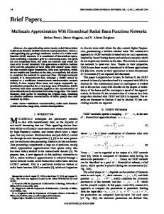
Figure 1: Left: RMS error versus the shape parameter from interpolating function (15). Right: condition numbers of the system matrix B versus the shape parameter. Although somewhat problem dependent, if a generalization could be made about the accuracy of RBF methods it would be that typically, the best 8
4
5
method d dd qd
|error| optimal ε time κ(B) 6.3e-9 1.85 4.9e-3 1.6e18 9.4e-14 1.05 3.1e-2 1.2e34 1.5e-21 0.55 3.0e-1 1.4e66
Table 3: Execution times, errors, and optimal shape parameters for interpolating function (15).
accuracy from RBF methods will be achieved with a shape parameter that results in a system matrix that is “critically conditioned” [6]. Critically conditioned means that the system matrix (or the evaluation matrix when solving steady PDE problems) has a condition number with the highest order of magnitude that varies smoothly as a function of the shape parameter. With the double type this range is κ(B) = O (1016 ). If, for fixed N, the shape parameter is decreased further, the calculated condition number will cease to be computed accurately and will oscillate between O (1017 ) and O (1020 ). Note that the optimal shape parameter, as we have defined it, may produce a system matrix with a condition number in the oscillatory range. For instance, in table 3 the optimal double shape parameter is listed as ε = 1.85, while the method is critically conditioned for approximately 4.0 ≤ ε ≤ 4.5. However, computational results from the oscillatory range are unpredictable. More reliable and “near optimal” results can be obtained from the critical range as can be seen in figure 1. With double-double precision the critically conditioned range is κ(B) = O (1032 ), and with quad-double the range is κ(B) = O (1064 ). The condition number rule of thumb applied to this situation would indicate that in the critically conditioned range for each floating point type that the calculated RBF expansion coefficients would have zero decimal places of accuracy. However, this is another instance where the errors are “diabolically correlated”, as the famous pioneering numerical analyst J. H. Wilkinson used to describe. The RBF expansion coefficients may not be accurately calculated when the method is critically conditioned, but compensating errors in other parts of the method result in the method being very accurate overall.
9
ε=5
0
0
10
10
qd dd d
−5
−5
10
RMS error
RMS error
10
−10
10
ε=2
−10
10
ε=1
−15
10
−15
10
−20
10
ε = 0.75
−20
10
0
−25
100
200 N
300
400
10
0
20
40
60
80
N
Figure 2: Left: RMS error versus the shape parameter from interpolating function (15). Right: RMS error versus N using quad-double precision and with various shape parameters. 4.1.2
fixed ε, refined N
In the left image of figure 2, the double calculation with ε = 5 has a steady error decay up to approximately N = 100 at which it has an O (10−8 ) error. However, due to the poor conditioning of the system matrix it is not possible to get further accuracy by increasing N. Double-double convergence begins to slow after N = 250, while the quad-double error continues to decay rapidly up to the largest N tested, which was N = 350. While extend precision allows RBF methods to be very accurate with large N (or small h), the most important benefit of extended precision with RBF methods may be the extreme accuracy that can be obtained with small N and relatively large minimum separation distance. This is illustrated in the right image of figure 2 with quad-double precision. With ε = 0.75 and N = 30 the error is O (10−10 ). With N = 60, 16 decimal places of accuracy are realized, and with N = 100 the error is O (10−24 ). 4.1.3
hybrid interpolation
Both N and ε may be varied in a hybrid approach which is often taken in applications. The shape parameter is adjusted with changing N so that the 10
100
system matrix remains critically conditioned (as described in section 4.1.1). In practice it is of course inefficient to calculate condition numbers so they are either estimated [16] or else a strategy is used to calculate the shape parameter, based on the minimum separation distance, that leads to the method being close to critically conditioned. Figure 3 illustrates the results 0
10
−5
RMS error
10
−10
10
−15
10
−20
10
d dd qd
−25
10
0
20
40
60
80
100
N
Figure 3: RMS error in interpolating function (15) versus N (hybrid interpolation) from interpolating function (15) using the three precisions with N varying from 10 to 100 in increments of 5. With the hybrid approach, convergence with double precision ceases at about N = 40 with an O (10−6 ) error. Above N = 40, the increase in shape parameter that corresponds to increasing N in order to prevent the system matrix from becoming too poorly conditioned also prevents any further increase in accuracy. The double-double error decay begins to cease about N = 60 with an O (10−14 ) error. The quad-double error is still decaying up to N = 100 and is approximately O (10−24 ). 4.1.4
mixed precision
All computations in the previous examples were carried out in the same precision. These include calculating the distance between centers, evaluating the 11
basis functions, solving the linear systems, and evaluating the interpolants. If accuracy of less than or equal to the fifteen decimal places afforded by double precision is desired, it may be questionable as to whether it is necessary to go to the expense of performing all calculations in extended precision. Is it possible to only solve the ill-conditioned systems (3) and (11) in extended precision and perform all other calculation in double precision? In some instances [17] mixed precision calculations have proven effective. This does not appear to be the case with RBF methods. In figure 4 the results are illustrated from using the standard double type to calculate the distance between centers, B, and f and the double-double type to calculate α. The expansion coefficients α are then converted to doubles and the interpolant is evaluated in double precision. Taking a mixed precision approach in this example reduces the accuracy to that comparable to an all double precision calculation. This can be explained by the fact that when the RBF methods become critically conditioned, the size of the expansion coefficients become very large. Evaluating the RBF interpolant involves summing the product of the expansion coefficients and basis functions which evaluate to small numbers when using small shape parameters. If the basis functions are not also evaluated using extended precision, the accumulated loss of accuracy from the coefficient by basis function product significantly decreases the accuracy of the approximation. For example, with N = 100 and ε = 1.05 which produces the smallest error with double-double precision in figure 1, the size of the expansion coefficients are O (1015 ).
4.2
2d Interpolation
As a two dimensional example we use the function 2 1 2 2 2 1 3 [ −1 3 −1 e 4 (9x−2) − 4 (9y−2) ] + e[ 49 (9x+1) − 10 (9y+1) ] 4 4 2 −1 2 2 2 1 [ −1 1 + e 4 (9x−7) − 4 (9y−3) ] − e[−(9x−4) −(9y−7) ] 2 5
f (x, y) =
(16)
that Franke [18] considered in his 1982 test of scattered data approximation methods. The function has become a standard test for scattered data interpolation methods. A surface plot of the function is shown in figure 6. The domain for the example is a circle of radius 0.25. In the example, the number of uniformly spaced centers N is increased from 30 to 390 in increments of 30. For each N, the interpolant is evaluated at M = 441 12
N = 100 mixed dd d
0
10
RMS error
−5
10
−10
10
−15
10
0
1
2 3 shape parameter, ε
4
5
Figure 4: Mixed floating point types. RMS error in interpolating function (15) versus the shape parameter. Mixing types results in comparable accuracy to double accuracy evaluation points. The RMS errors and execution times are recorded in table 4. Figure 5 illustrates the center and evaluation point layout with N = 60. Figure 7 shows the RMS error versus the shape parameter using N = 300. If eight accurate decimal places are desired, the accuracy can be achieved with either a double computation with N = 330 in 3.9e-2 second or with a double-double computation with N = 120 in 0.1 second. If extreme accuracy, such as fourteen decimal places is desired, quad-double precision with N ≥ 300 must be used. Approximately one decimal place of accuracy is gained with each addition of 30 centers until the system (3) becomes too poorly conditioned for the trend to continue. The trend continues until N = 90 with the double type, indicating that for larger N the condition number of the system matrix is above O (1016 ). The convergence trend continues until N = 300 with the double-double type which indicates that for larger N the condition number of the system matrix is above O (1032 ). With all N used (up to N = 390) the trend continues with quad-double precision indicating that the condition number of the system matrix remains under O (1064 ). 13
N = 60 0.3 0.2
y
0.1 0 −0.1 −0.2 −0.2
0 x
0.2
Figure 5: N = 60 centers marked with asterisks and M = 441 evaluations points marked with dots for the Franke function (16) interpolation example.
4.3
Extended Precision versus “bypass” algorithms
The term bypass algorithm refers to an algorithm that evaluates a RBF approximation without solving the linear system (3) or (11). Methods that work with the linear systems are usually called direct methods. In [19], an algorithm called the Contour-Pad´e (cp) algorithm is described for evaluating RBF approximation methods that avoids working directly with the associated ill-conditioned linear systems. The algorithm stably calculates the RBF approximant for small values of the shape parameter ε that cannot be handled by direct methods using double precision. The algorithm is severely limited by the restriction that it only works with a small number of centers (usually N < 80). Next we use an example to compare the Contour-Pad´e algorithm to the direct method with extended precision. We approximate the first order partial derivative with respect to x of the function f (x, y) = exp(x/2+y/4) using the 60 scattered centers in figure 8. The approximation is evaluated at the center that is located at approximately (0.7487,-0.1156) and is marked with an asterisk in figure 8. The resulting error plots versus the shape parameter are shown in figure 9. The execution times, RMS errors, and optimal shape parameters for the example are in table 5. Both the double-double and quaddouble extended precision direct methods are more accurate in this example than the Contour-Pad´e algorithm. 14
N 30 60 90 120 150 180 210 240 270 300 330 360 390
execution time, secs d dd qd 1.6e-3 2.0e-2 2.6e-1 2.2e-3 3.5e-2 5.2e-1 2.8e-3 6.4e-2 8.9e-1 3.8e-3 1.0e-1 1.3 1.0e-2 1.6e-1 2.0 7.5e-2 1.9e-1 2.5 1.1e-2 3.3e-1 4.0 1.5e-2 4.7e-1 5.4 2.1e-2 6.2e-1 7.0 2.5e-2 8.3e-1 9.0 3.9e-2 1.0 11.4 4.4e-2 1.3 14.2 4.6e-2 1.6 17.5
RMS d 2.0e-4/1.6 5.8e-5/1.05 6.7e-7/1.5 5.9e-7/1.5 1.9e-7/1.55 7.0e-8/2.2 2.3e-8/2.5 2.8e-8/2.55 1.2e-8/2.75 1.3e-8/2.35 8.4e-9/2.85 8.3e-9/2.8 5.3e-9/2.8
error/optimal dd 2.0e-4/1.6 5.7e-5/1.05 1.7e-7/1.3 8.9e-9/1.0 1.7e-9/0.95 2.5e-10/0.85 1.2e-11/0.95 2.8e-12/1.05 1.4e-12/1.0 5.4e-13/1.4 4.6e-13/1.2 5.9e-13/1.4 2.6e-13/1.45
shape qd 2.0e-4/1.6 5.7e-5/1.05 1.7e-7/1.3 8.9e-9/1.0 1.7e-9/0.95 2.5e-10/0.85 1.2e-11/0.95 9.8e-13/0.8 1.4e-13/0.7 6.0e-15/0.75 1.5e-15/0.75 1.3e-16/0.7 5.6e-17/0.8
Table 4: Execution times, RMS errors, and optimal shape parameters for the 2d interpolation example using the Franke function (16)
method d cp dd qd
|error| optimal ε time 3.2e-7 0.175 2.9e-3 7.2e-10 0.120 3.8e-1 9.5e-11 0.08 1.2e-2 8.9e-11 0.005 1.4e-1
Table 5: Execution times, errors, and optimal shape parameters for the first bypass algorithm example. See figure 9 for more information.
15
1.1 1 0.9 0.8 0.7 0.6 0.5 0.4 0.5 0.4
0.2
0
0
−0.2
−0.4
−0.5
y
x
Figure 6: Franke’s function. A second bypass algorithm is the RBF-QR method. The RBF-QR algorithm [20] stably evaluates RBF methods in the special case of when the domain is the surface the surface of a sphere. Unlike the Contour-Pad´e algorithm, the RBF-QR algorithm is not limited to a small number of centers. In [21], the RBF-QR algorithm is extended to work with Gaussian RBFs in two dimensions. For accuracy and use with large N, the 2d RBF-QR algorithm requires the use of extended precision. If double-double precision arithmetic is used within the algorithm, the upper limit on N is about 2700 centers. If accuracy of the order O (10−6 ) is sufficient, the limit goes up to about 6000 centers if double-double precision floating point arithmetic is used. We test the RBF-QR algorithm with the largest N that was used with the Franke function example. We use the Matlab version of the RBF-QR algorithm that is available electronically on the web site of the second author of reference [21]. The RBF-QR algorithm executes in 465 seconds with N = 390, ε = 1.45, and has an RMS error of 2.9e-12. For comparison, the C++ code using double-double precision with N = 390 and ε = 1.45 executes in 1.6 seconds and has an RMS error of 2.6e-13. An efficiently written C++ version of the RBF-QR algorithm would improves it’s efficiency, but in the code that
16
N = 300
0
10
d dd qd −5
RMS error
10
−10
10
−15
10
1
2
3
shape parameter, ε
4
5
Figure 7: RMS errors versus the shape parameter for the Franke function interpolation example with N = 300. is publicity available the algorithm programmed in Matlab does not seem viable for use in applications. The C++ extended precision double-double direct method code is 290 times faster as well as slightly more accurate.
4.4
Steady PDEs
As a two dimensional steady PDE example we consider the Poisson problem uxx + uyy = (λ2 + µ2 )e(λx+µy) , (x, y) ∈ Ω (λx+µy) u(x, y) = e , (x, y) ∈ ∂Ω
(17)
with λ = 1, µ = 2, and a domain Ω taken to be the unit circle. The exact solution is u(x, y) = e(λx+µy) . The accuracy results, execution times, and optimal shape parameters for problem (17) are listed in table 6 for various N and three floating point precisions. The N centers are uniformly spaced as shown for N = 300 in figure 10. In this example, increasing precision from double to double-double results in execution times being approximately 10 times slower. Increasing 17
1 0.5 0 −0.5 −1 −1.5
−1
−0.5
0
0.5
1
1.5
Figure 8: The Contour-Pad´e algorithm evaluates ∂f /∂x at the center marked with the asterisk and is compared to the accuracy of the direct method with various floating point precisions.
−4
10
−6
|error|
10
−8
10
cp d dd qd
−10
10
0
0.1 0.2 shape parameter, ε
0.3
Figure 9: Standard and extended precision Gaussian Elimination and Contour-Pad´e error versus the shape parameter for approximating ∂f /∂x of function f (x, y) = exp(x/2 + y/4) at the point (0.74874,-0.11558) that is marked in figure 8.
18
execution time, secs RMS error/optimal N d dd qd d dd 20 3.9e-4 1.8e-3 1.6e-2 3.1e-2/0.035 2.5e-2/0.003 30 5.9e-4 3.9e-3 4.1e-2 2.9e-3/0.1 2.1e-3/0.008 60 1.7e-3 2.0e-2 1.9e-1 4.8e-4/0.2 8.2e-5/0.04 75 2.8e-3 3.0e-2 3.1e-1 6.4e-4/0.23 3.1e-5/0.08 90 5.6e-3 4.7e-2 4.9e-1 1.7e-4/0.3 3.7e-6/0.08 150 1.7e-2 1.7e-1 1.7 1.1e-4/0.42 2.3e-8/0.18 225 4.8e-2 4.9e-1 4.7 3.6e-5/0.55 3.7e-9/0.17 300 1.0e-1 9.2e-1 9.7 5.4e-5/0.58 1.3e-9/0.2 400 2.3e-1 2.3 1.0e-5/0.75 3.2e-10/0.27 500 4.3e-1 4.1 8.0e-6/0.76 2.1e-10/0.27 1000 3.3 29.2 5.9e-6/1.23 1.9e-11/0.39
shape qd 2.1e-2/0.002 2.1e-3/0.0001 5.0e-5/0.02 5.4e-6/0.03 9.6e-7/0.04 2.0e-10/0.08 3.9e-14/0.04 0/0.06 -
Table 6: Execution times, RMS errors, and optimal shape parameters for the steady PDE problem 17
precision from double-double to quad-double results again results in a factor of 10 execution penalty. With a goal of five accurate decimal places, doubledouble with N = 90 is the most efficient choice with an error of 3.7e-6 and an execution time of 4.7e-2 seconds. To obtain five accurate decimal places with double precision we need N = 500 which executes in 4.3e-1 seconds. If more than five accurate decimal places are desired, double-double or quad-double precision must be used as the goal can not be achieved in double precision. With N = 300 (right image of figure 11) the quad-double calculation is accurate to more than 16 decimal places. In this example we did not record accuracy results of more than 16 decimal places. In table 6 we see the extreme accuracy that is possible when using extended precision. However, many scientists and engineers do not need RMS errors on the order of machine epsilon, but rather just several decimal places of accuracy. In our final experiment, we consider some moderate error goals between 1e-3 and 1e-7 and find the minimum N needed to achieve the accuracy goal. The results along with execution times are recorded in table 7. If an error of no more that 1e-3 can be tolerated, the standard double precision calculation is the most efficient. However, with the four other more stringent accuracy goals, the double-double calculations are the most efficient. When using standard double precision, the two most stringent accuracy goals can 19
N = 300 1
y
0.5
0
−0.5
−1 −1
−0.5
0 x
0.5
1
Figure 10: N = 300 centers for the 2d Poisson problem (17). not be achieved.
5
Conclusions
In summarizing the current state of and the evolution of computer technology and floating point arithmetic, the author of reference [15] concludes that “Inevitably, 256-bit floating point will become the standard eventually.” RBF methods will certainly benefit in the future from this predicted hardware accuracy goal 1e-3 1e-4 1e-5 1e-6 1e-7
N execution time, secs d dd qd d dd qd 53 38 38 1.6e-3 4.0e-3 4.2e-2 196 53 53 4.5e-2 9.2e-3 9.3e-2 490 79 71 4.3e-1 3.2e-2 2.0e-1 105 90 6.3e-2 4.9e-1 145 105 1.6e-1 7.3e-1
Table 7: The number of centers needed to meet accuracy goals and the execution times for the steady PDE problem 17.
20
N = 150
5
N = 300
10
0
d dd qd
d dd qd
10
0
RMS error
RMS error
10
−5
10
−5
10
−10
10
−10
10
0
0.2
0.4 0.6 0.8 shape parameter, ε
1
0
0.2
0.4 0.6 0.8 shape parameter, ε
Figure 11: RMS errors versus the shape parameter for the steady PDE problem (17). Left: N = 150. Right: N = 300. implementation of more accurate floating point arithmetic. Until processors evolve to handle such precision in hardware, the RBF method can benefit from efficiently implemented software extended precision. The high computational overhead associated with arbitrary precision with large dps ≥ 100 results in tools that currently are not efficient enough to be used in most applications. Fortunately, the extended precision double-double and quad-double types can be implemented more efficiently and are able to dramatically improve the accuracy of the RBF methods. In the numerical experiments, double-double calculations took approximately 10 times longer to execute than double calculations, and quad-double 10 times longer than double-double. However, reference [1] reports that it is more typical for double-double calculations to take 5 times longer than double calculations, and quad-double to 5 times longer than double-double. The difference in results is most likely due to the choice of compilers or choice of optimization flags. If extreme accuracy is desired and if the theoretical spectral convergence rates are to be achieved, extended precision is a must. In many cases using extended precision may even be more efficient. Extended precision may produce a smaller error with small N and execute more quickly than standard precision software with large N. This was the case in our steady PDE exam21
1
ple. Domain decomposition will be an important tool to use with extended precision on higher dimensional problems in order to keep N sufficiently small so that the extended precision execution times are comparable to standard precision times with larger N. Mixing numerical precisions, e.g., solving the ill-conditioned linear systems (3) and (11) in extended precision while performing all other computations in double precision, did not improve on standard double precision results in our examples. A typical result of using mixed precision was given in section 4.1.4. All parts of the approximation must take place in extended precision in order to reap accuracy benefits. The availability of a C++ extended precision RBF package that calculates distance matrices, evaluates basis functions and their derivative, performs necessary linear algebra, etc., would undoubtedly be beneficial to the development of RBF methods and further increase the popularity and application of the methods. Bypass algorithms evaluate the RBF approximate without directly work with the linear systems (3) and (11). The Contour-Pad´e algorithm is applicable in the case of a small numbers of centers. In our numerical example the double-double solution of linear system was more accurate than the Contour-Pad´e algorithm using double precision. Extended precision could be used within the Contour-Pad´e algorithm as well, but the algorithm includes the solution of multiple linear systems and using extended precision would increase the execution time dramatically. The other bypass algorithm, the RBF-QR method was not as accurate as the direct double-double method for the Franke function example and the execution time of the RBF-QR method in this example indicated it was not viable for use in applications. In [21], the authors suggest that the algorithm be implemented with extended precision with large N in order to improve accuracy. However, performing the QR factorization within the method in extended precision would further increase the execution time. One of the most attractive features of RBF methods is their simplicity. Working with the RBF method is as simple as setting up and evaluating a linear system. While the mathematics of the bypass algorithms are interesting and often elegant, they add a great deal of complexity to the RBF method in order to recast an ill-conditioned linear system in a different light. Our experience suggests that the rather inelegant and brute force approach of extend precision is much easier to implement and also often more accurate and efficient. In this work, we have examined the costs and benefits of using extended precision floating point arithmetic in RBF interpolation methods and in RBF 22
methods for steady PDEs. Many questions remain about eigenvalue stability for RBF methods for time-dependent PDEs [22, 23]. Extended precision may be of benefit to RBF methods for time-dependent PDEs and will be explored in future work. Additionally, it has been previously suggested by the second author in [6] that RBF methods are an appropriate tool for the numerical solution of high dimensional (d ≥ 4) PDEs. The use of extended precision with RBF methods may afford the use of relatively small N to achieve moderate accuracy for this class of problem.
References [1] D. H. Bailey. High-precision arithmetic in scientific computation. Computing in Science and Engineering, pages 54–61, 2005. 1, 3, 5 [2] D. H. Bailey and Jonathan M. Borwein. High-precision computation and mathematical physics. To appear in XII Advanced Computing and Analysis Techniques in Physics Research, 2008. 1 [3] C.-S. Huang, C.-F. Leeb, and A.H.-D. Cheng. Error estimate, optimal shape factor, and high precision computation of multiquadric collocation method. Engineering Analysis with Boundary Elements, 31:614–623, 2007. 1 [4] D. Bailey, Y. Hida, X. Li, and B. Thompson. High precision software. http://crd.lbl.gov/ dhbailey/mpdist/. 1, 3 [5] E. J. Kansa. Multiquadrics - a scattered data approximation scheme with applications to computational fluid dynamics II: Solutions to parabolic, hyperbolic, and elliptic partial differential equations. Computers and Mathematics with Applications, 19(8/9):147–161, 1990. 2 [6] S. A. Sarra and E. J. Kansa. Multiquadric Radial Basis Function Approximation Methods for the Numerical Solution of Partial Differential Equations. Tech Science Press, 2010. 2, 4.1.1, 5 [7] M. D. Buhmann. Radial Basis Functions. Cambridge University Press, 2003. 2 [8] G. E. Fasshauer. Meshfree Approximation Methods with Matlab. World Scientific, 2007. 2 23
[9] H. Wendland. Scattered Data Approximation. Cambridge University Press, 2005. 2 [10] C. Micchelli. Interpolation of scattered data: Distance matrices and conditionally positive definite functions. Constructive Approximation, 2:11–22, 1986. 2 [11] Y. C. Hon and R. Schaback. On unsymmetric collocation by radial basis function. Applied Mathematics and Computations, 119:177–186, 2001. 2 [12] W. R. Madych and S. A. Nelson. Bounds on multivariate interpolation and exponential error estimates for multiquadric interpolation. Journal of Approximation Theory, 70:94–114, 1992. 2 [13] L. N. Trefethen and D. Bau. Numerical Linear Algebra. SIAM, first edition, 1997. 2, 4 [14] R. Schaback. Error estimates and condition numbers for radial basis function interpolation. Advances in Computational Mathematics, 3:251– 264, 1995. 2 [15] M. Overton. Numerical Computing with IEEE Floating Point Arithmetic. SIAM, 2001. 3, 5 [16] J. Demmel. Applied Numerical Linear Algebra. SIAM, 1997. 4.1.3 [17] X. S. Li, J. W. Demmel, D. H. Bailey, and G. Henry. Design, implementation and testing of extended and mixed precision BLAS. ACM Transactions on Mathematical Software, 20(2):152–205, 2002. 4.1.4 [18] R. Franke. Scattered data interpolation: Tests of some methods. Mathematics of Computation, pages 181–200, 1982. 4.2 [19] B. Fornberg and G. Wright. Stable computation of multiquadric interpolants for all values of the shape parameter. Computers and Mathematics with applications, 48:853–867, 2004. 4.3 [20] B. Fornberg and C. Piret. A stable algorithm for flat radial basis functions on a sphere. SIAM Journal of Scientific Computing, 30:60–80, 2007. 4.3
24
[21] B. Fornberg, E. Larsson, and N. Flyer. Stable computations with Gaussian radial basis functions in 2-d. Submitted to SIAM Journal of Scientific Computing, 2009. 4.3, 5 [22] R. Platte and T. Driscoll. Eigenvalue stability of radial basis functions discretizations for time-dependent problems. Computers and Mathematics with Applications, 51:1251–1268, 2006. 5 [23] S. A. Sarra. A numerical study of the accuracy and stability of symmetric and asymmetric RBF collocation methods for hyperbolic PDEs. Numerical Methods for Partial Differential Equations, 24(2):670 – 686, 2008. 5
25