we are considering a set of images whose elements have the same value almost ... because it tells us that we do not have much information to work with. .... ment vector, v, and vector direction (cos θ, sin θ) (blue col- ored curve). ... panel Ω. 1 . For the set of frequencies in Ω. 1. , cos θ = 0, we can write: Ëfd[n, m] = â j,k f[j, k]e.
Radon Transform for Lineal Symbol Representation Oriol Ramos Terrades∗, Ernest Valveny† Computer Vision Center - Dept. Inform`atica Universitat Aut`onoma de Barcelona Edifici O - Campus UAB, 08193 Bellaterra, SPAIN {oriolrt,ernest}@cvc.uab.es Abstract Content-based retrieval and recognition of graphic images requires good models for symbol representation, able to identify those features providing the most relevant information about the shape and the visual appearance of symbols. In this work we have used the Radon transform as the basis to extract the representation of graphic images as it permits to globally detect lineal singularities in an image, which are the most important source of information in these images. The image obtained after applying Radon transform can be used directly to describe the symbol, or can be used to extract new and compact descriptors from it, which will also be based on lineal information about the image. We present some preliminary results showing the usefulness of this representation with a set of architectural symbols.
1. Introduction Images of graphic symbols use to be very structured, with only few particular features allowing to describe them. Lines and arcs of circumference are usually the most common curves we can find into a drawing. More complex curves are rare. If we consider such lines being of zerowidth, we can observe that this kind of images have zeronorm, in any Lp norm, i.e. from an analytic point of view, we are considering a set of images whose elements have the same value almost everywhere, except for the very small set corresponding to lines. This is a very remarkable property because it tells us that we do not have much information to work with. Moreover, all relevant information is concentrated in a small set of singularities where the image is non-zero, usually one in binary images. Thus, if we want to get a useful representation of linear images, we must be able ∗ Supported † Partially
by UAB grant supported by CICYT TIC2000-0382, Spain
to accurately identify and describe those singularities corresponding to their geometric features. Good symbol representation is the basis for a lot of applications working with graphic images, such as indexation and content-based retrieval in databases of document images, graphic web navigation or symbol recognition. Vectorization[4, 6, 7, 10] has usually been used to extract line information in graphic images. These methods usually work only with local information and are very noise sensitive and dependent on accurate tuning of a set of parameters. As different symbols have different number of lines, it is difficult to find an homogeneous representation easy to compare and to use in retrieval operations. In this work we explore another way to identify and represent line information applying a global transformation to the image which will provide an homogenous representation for all symbols. In this sense, if we try to determine image singularities by computing the modulus and the phase of image gradient we obtain images where it is difficult to work. We obtain images very similar in its structure to the original image. Therefore, we must think of another strategy. We should have a mathematical transform which converts line singularities in original images into characteristic points in the transformed image. These points should be local maxima in order to be able to extract them with some post-process. Radon transform, RT, appears to be a good candidate. Radon transform converts original image into a new image space with parameters θ and t. Each point in this new space accumulates all information corresponding to a line in the original image with angle θ and radius t. Thus, when Radon transform localizes near an angle θ0 and around a slice t0 a local maximum it results that original image has a line in position (t0 , θ0 ). This is the kind of transform we are looking for. In this paper, we show how Radon transform efficiently represents and geometrically describes linear symbols. We briefly resume Radon transform and its properties in section 2. Then, in section 3, we present Fast Radon transform (de-
Proceedings of the Seventh International Conference on Document Analysis and Recognition (ICDAR 2003) 0-7695-1960-1/03 $17.00 © 2003 IEEE
veloped by Averbuch et al. [1]) and discuss some geometrical precision problems it has and how we have solved them. Finally, sections 4 and 5 describe experimental studies and gives a discussion about advantages and limitations of our approach applied to the representation of linear symbols.
2
Radon Transform
(a)
(b)
(c)
(d)
For a L2 function f (x), let Rf denote the Radon transform of f , which is defined as the integral of the function along a line Lt,θ , and is expressed using the Dirac mass δ: � Rf (t, θ) = f (x1 , x2 )δ(x1 cos θ + x2 sin θ − t)dx, (1) where our phase space is R × [0, 2π). In binary images, the Radon transform value at point (t0 , θ0 ) will be the total length of all segments belonging to line Lt,θ . Radon transform has some interesting properties relating to the application of affine transformations. We can compute the Radon transform of any traslated, rotated or scaled image, knowing the Radon transform of the original image and the parameters of the affine transformation applied to it. This is a very interesting property for symbol representation because it permits to distinguish between transformed objects, but we can also know if two objects are related by an affine transformation by analyzing their Radon transforms. Let’s see these three properties: • Rotation Let Gα be the rotation of angle α, which is applied to an image f (x). Then, the Radon transform of the rotated image can be expressed as: R (f ◦ Gα (x)) (t, θ) = Rf (t, θ + α). • Shift Let Tv (x) = x + v, v ∈ R2 , be the traslation of an image. Then the Radon transform of the traslated image is: R (f ◦ Tv (x)) (t, θ) = Rf (t + t� (θ), θ), where t� (θ) = v1 cos(θ) + v2 sin(θ). • Scale Let Ha (x) = ax, a > 0, be the scaling of an image. Then, the Radon transform of the scaled image is: R (f ◦ Ha (x)) (t, θ) =
1 Rf (at, θ), a
The effect of rotation on Radon transform can be seen in figures 3.a and 3.c. We can see how, as images are being more rotated, local maxima of Radon transform move to the right, while slice t remains constant, i.e., the Radon transform of rotated images is the same as the original, but shifted in the angular direction by the angle of rotation.
Figure 1. Shifts effects. Shift effect is quite interesting because it tell us that angular parameter is independent to shift. However, slice parameter depends on the shift and θ. Horizontal shifts don’t affect horizontal segments’ Radon transform (figure 1). Shift contribution t� is the inner product between movement vector, v, and vector direction (cos θ, sin θ) (blue colored curve). There exist two digital implementations of Radon transform: direct and Fourier implementation. Direct strategies [3] try to optimize calculus of equation 1. Averbuch et al. [1] proposes a fast method to implement Discret Radon transform DRT based on the Fourier strategy.
3
Fast Discret Radon Transform
Fourier Slice theorem gives us the relationship between Radon transform and Fourier transform [9]. Let us denote F1 , F2 the univariate and bivariate, respective, Fourier transform and the polar-to-cartesian operator P . Then: F1 ◦ R = P ◦ F2
(2)
This expression suggests us a two steps method to estimate the Radon transform of an image. Firstly, we can calculate Polar Fourier transform, the right side in equation (2) and after that, we can apply inverse 1D Fourier transform to recover Radon transform. From the 2-dimensional discret Fourier’s expression, we get: � f [j, k]e−i(kω1 +jω2 ) (3) fˆd (ω1 , ω2 ) = j,k
we can change this expression to polar coordinates by writing ω1 = ξ cos θ and ω2 = ξ sin θ. Then, we replace in (3) n , n = 0, . . . , N − 1 and θm = 2π by sampling ξn = N M m, m = 0, . . . , M − 1.
Proceedings of the Seventh International Conference on Document Analysis and Recognition (ICDAR 2003) 0-7695-1960-1/03 $17.00 © 2003 IEEE
3
2
1
a) 0
−1
−2
b) −3 −3
−2
−1
0
1
2
3
Figure 2. Pseudopolar grid for N = 8 fˆd [n, m] =
�
− in N (k cos
f [j, k]e
2πm M +j
sin
2πm M
)
c)
(4)
Figure 3. a) rotated images. b) Local maximums near angles π4 move away from red line. c) corrected version
j,k
It is not clear how to calculate equation (4) in a fast way. However, Averbuch et al. define a pseudopolar grid (see figure 2), where circumferences are approximated by squares in order to have frequencies aligned in two separate panels: the first one, Ω1 , is composed of frequencies with angles in [− π4 , π4 ) and the second one composed of those frequencies 2 with angles in [ π4 , 3π 4 ), Ω . Ω1 = Ω2 =
�� ��
nπ nπ 2 , m N M N 2 nπ nπ m , M N N
� − N ≤ n < N, −
M M ≤m< 2 2
− N ≤ n < N, −
M M ≤m< 2 2
�
� �
We are going to develop Averbuch et al. approach with panel Ω1 . For the set of frequencies in Ω1 , cos θ = 0, we can write: � fˆd [n, m] = f [j, k]e−iξ cos θ(k+j tan θ) j,k
and tan θ = 2m M . Thus: � π 2m fˆd [n, m] = f [j, k]e−i N n(k+j M )
But ξ cos θ =
nπ N
j,k
=
� � � j
Setting αm =
� π −i N nk
f [j, k]e
2π
2m
e−i N nj M
k
2m NM ,
we rewrite this last expression as: � � � � π fˆd [n, m] = f [j, k]e−i N nk e−i2πnjαm , j
This discrete implementation results in a Radon transform that is geometrically exact to the continuous version in the same way circles are similar to square. There is some distortion form ideal transform introduced by the use of a pseudo-polar grid instead of using a real polar grid. Figure 3.b shows what we mean. As we move away from origin, the distance between image transform local maxima and theoretical local maxima grows. The red line corresponds to the position in t direction where all maxima should be. However, for rotated images, local maxima are farther from the origin. Furthermore, slice parameter t and angular parameter θ, are not uniformly sampled for all couple (t, θ). We have developed a slightly different implementation of the Discrete Radon Transform, where we correct the sampling of t parameter and we increase geometrical precision by replacing the last 1D inverse Fourier transform in equation 2 by its fractional version with parameter α according to the angular value in each column. In the pseudopolar grid, for each angle θ, t samples are equispaced but distances between them depends on the angle. Fractional Fourier transform allows us to obtain an uniform t sampling for all θ, as we can see in figure 3.c, where all local maxima are located at the same value of parameter t, independently of the angle. As angular sampling is not important for our applications, we leave it as in Averbuch et al. approach.
(5)
k
where external sum is a Fractional Fourier transform with parameter αm , that can be computed with logarithmic cost, [2]. Panel Ω2 can be treated in an analogous way, replacing cos by sin and tan by cot. In this way, we can compute the right side of equation 2. Finally, we only have to apply 1D inverse Fourier transform to each column and we retrieve the Radon Transform.
4
Experiments and discussion
We have used a set of seven different linear symbols to test the validity of the Radon transform to represent them. Figure 4 shows these symbols and their Radon transform. We have scaled every image in such a way that one bounding box side had length 64 and we have centered it in an 64 × 64 image. We could distinguish two different
Proceedings of the Seventh International Conference on Document Analysis and Recognition (ICDAR 2003) 0-7695-1960-1/03 $17.00 © 2003 IEEE
0
12.19
4.90
7.63
85.43
84.77
71.60
1.76
0
1.07
1.02
100
99.53
82.20
7.53
5.75
0
6.12
90.68
90.23
72.09
2.63
1.48
0.58
0
89.20
88.11
73.03
8.23
6.41
5.718
3.27
0
0.27
0.18
8.21
7.68
3.71
1.67
0.27
0
0.01
8.78
6.07
3.09
5.05
4.45
4.34
0
Figure 5. Distance between symbols Figure 4. Symbols used ant its Radon Transform
groups of symbols. The first one is composed of figures containing a rectangle: symbols 1,2,3 and 4. Essentially, in such symbols we add a variety of linear structures to a rectangle. The second group is a collection of arrow symbols. Differences among the elements on this group are minima. From the analysis of the Radon transform of these images, we can observe that all images sharing a common structure such as the rectangle have also a common structure in its Radon transform corresponding to the lines of the rectangle. All images having similar lines in orientation and position have the same maxima in the Radon transform. In this way we show how the Radon transform is able to capture the lineal information of the symbols. Moreover, symbols belonging to the second group, which are very similar in their visual appearance have almost the same Radon transform. In order to measure the power of Radon transform in capturing symbol similarities and differences we have defined a “non-symmetric distance” d. Let us denote sl our symbol collection, l = 1, . . . , 7, and sl (j) the map that return the j-th local maximum’s coordinates of symbol l. Then we define d(sn , sm ) as: d(sn , sm ) =
Nm 1 � min {�sn (i) − sm (j)�2 } (6) Nm j=1 i=1,...,Nn
where Nl is the number of representative lines for symbol sl . This “non-symmetric distance” gives us an inclusion relationship between symbols. Let us denote dn,m = d(sn , sm ). Then, dn,m < dm,n implies that sn structure is in sm structure. For example, if we compare a square, Sq, with one of its sides, S: 0 = d(S, Sq) < d(Sq, S) (replacing in (6)), so one square’s side belongs to square. This
property of the distance and the Radon transform permits to identify symbols with a common structure. We have also define a symmetric distance between symbols to compare them. An easy way to construct a symmetric distance from the previous one is to define:
D(sn , sm ) =
1 (dn,m + dm,n ) 2
(7)
To compute this distance we must extract, from Radon transform, the location of every significant segment in the image. As Radon transform gives us information about the length of segments in a given location, if we choose an appropriate threshold we can select locations in the Radon space corresponding to significant lines in the image space. However, due to noise, each line will be represented by a distribution of points centered on the segment location. To find the exact location of every segment, we have applied a gaussian mixture to the thresholded image to get the center of each distribution. Table 5 shows the matrix of non-symmetric distances among all the symbols. This distances have been normalized in the range [0, 100], according to he maximum value, in order to make easier comparatives. We can see how the symbols in group one have lower distances among them than with symbols in group two. This is due to the fact that all symbols in this group share a common structure around a rectangle. We also observe how distances among symbols in group 2 are the lowest, corresponding to the fact that their similar appearance is very similar. Finally, if we analyze information provided by the asymmetry of the distance, we can see that the distance complies with the inclusion relationship explained before. Symbols in group 2 can be included in symbols of groups 1. Thus, distances are lower in this direction than in the opposite one. In the same way, symbol 2 which can be included in the other symbols
Proceedings of the Seventh International Conference on Document Analysis and Recognition (ICDAR 2003) 0-7695-1960-1/03 $17.00 © 2003 IEEE
have lower distances in the direction from this symbol to the other ones. Finally, we have carried out an experiment to test the robustness of the representation obtained with the Radon transform to shape distortions. We have taken fifty handdrawn images of symbol 1 with a high degree of distortion from the ideal shape of the symbol. For each image, we have found using the procedure explained before with an appropriate threshold, the location in the Radon space of all significant lines in the image space corresponding to all the images. We have plot all points in a single image getting a distribution of locations for each line and we have applied a gaussian mixture to get the center of each distribution. We can see it in figure 6. It shows how, despite of the distortion the local maxima corresponding to each line are close for all images. The black point in each distribution is the location of the line in the ideal model. We can see how it is located inside the area of influence of each distribution, showing that it captures well the information of every line. In order to verify if our distance defined in (7) catches well our perception, we have computed the distance between the new representation got from the distorted symbols and every model, showing us that the ideal model of the symbol 1 is the closest to noisy images, whereas the others models are well distinguished by the distance - figure 6 -. 250
200
150
100
50
0
4.34
0
33.40
50
25.64
100
32.00
150
200
100
250
99.21
76.86
Figure 6. Representation of distorted images
5
Conclusions and future work
A good representation of images is the basis for any application concerning matching, retrieval, browsing or recognition. In this work we have explored the possibilities of Radon transform in order to get such representation. Radon transform converts the original image into a new one, with local maxima at points corresponding to the parameters θ and t of the lines, taken as singularities in the image space. Application of Radon transform to a set of graphic images shows that it is able to capture shape structure of sym-
bols and that it is robust to unconstrained shape distortions. Symbols with a common structure share maxima location in the Radon transform, although the Radon transform also reflects differences among them. Then, it can be used to distinguish among different symbols, but also to search similar symbols. The non-symmetric similarity measure d can be used to decompose any symbol in primitive shapes, obtaining a high level feature vector and reducing symbol database size. However, it is essential to have an accurate description of primitive symbols. In that way, works such as [5, 8], where singularities in the Radon space are detected using Ridgelets transform, could enlighten in that direction. Distorted shapes os a symbol result in a Radon transform which has the same global structure than the ideal one, with few differences in the location of significant points. Properties of Radon transform permit to handle affine transformations from the Radon transform of the original image. These results must be taken as a preliminary study in the way of getting a general representation model for symbols. From Radon transform of an image we must consider extracting a set of descriptors keeping shape information and easy to compute and to compare.
References [1] A. Averbuch, R. Coifman, D. Donoho, M. Israeli, and W. J. Fast slant stack: A notion of radon transform for data in a cartesian grid which is rapidly computible, algebraically exact, geometrically faithful and invertible. 2001. [2] D. H. Bailey and P. N. Swarztrauber. The fractional fourier transform and aplicattions. SIAM Review, 33(3):389–404, September 1991. [3] M. L. Brady. A fast discret approximation algorithm for the radon transform. SIAM J. Comput, 27(1):107–119, February 1998. [4] Y. Chen, N. Langrana, and A. Das. Perfecting vectorized mechanical drawings. Computer Vision and Image Understanding, 63(2):273–286, March 1996. [5] D. L. Donoho. Orthonormal ridgelets and linear singularities. 2001. [6] D. Dori and W. Liu. Sparse pixel vectorization: An algorithm and its performance evaluation. IEEE Trans. on PAMI, 21(3):202–215, March 1999. [7] V. Nagasamy and N. Langrana. Engineering drawing processing and vectorisation system. Computer Vision, Graphics and Image Processing, 49:379–397, 1990. [8] O. Ramos and E. Valveny. Line detection using ridgelets transform for graphic symbol recognition. In Proceedings of First IbPRIA, June 2003. Andratx, Spain. To appear. [9] A. Rosenfeld and A. C. Kak. Digital Picture Processing. Academic Press, San Diego, California, 1982. [10] K. Tombre, C. Ah-Soon, P. Dosch, G. Masini, and S. Tabonne. Stable and robust vectorization: How to make the right choices. In Proceedings of Third IAPR Work. on Graphics Recognition, pages 3–16, Sept 1999. Jaipur, India.
Proceedings of the Seventh International Conference on Document Analysis and Recognition (ICDAR 2003) 0-7695-1960-1/03 $17.00 © 2003 IEEE