Random Forests of Very Fast Decision Trees on GPU for Mining ...

Random Forests of Very Fast Decision Trees on GPU for Mining Evolving Big Data Streams Diego Marron1 and Albert Bifet2 and Gianmarco De Francisci Morales3 Abstract. Random Forest is a classical ensemble method used to improve the performance of single tree classifiers. It is able to obtain superior performance by increasing the diversity of the single classifiers. However, in the more challenging context of evolving data streams, the classifier has also to be adaptive and work under very strict constraints of space and time. Furthermore, the computational load of using a large number of classifiers can make its application extremely expensive. In this work, we present a method for building Random Forests that use Very Fast Decision Trees for data streams on GPUs. We show how this method can benefit from the massive parallel architecture of GPUs, which are becoming an efficient hardware alternative to large clusters of computers. Moreover, our algorithm minimizes the communication between CPU and GPU by building the trees directly inside the GPU. We run an empirical evaluation and compare our method to two well know machine learning frameworks, VFML and MOA. Random Forests on the GPU are at least 300x faster while maintaining a similar accuracy.

With the raise of GPUs as a general purpose platform that provides high throughput computation, researchers have started to explore their use in high performance data mining. Deep Learning is an example of a hugely successful application of GPUs to large scale batch learning [4]. Therefore, it is interesting and challenging to see whether and how we can draw benefits from such an architecture in a streaming context. In this work, we focus on one of the most common data mining applications: classification. In particular, we study how to effectively deploy decision trees and random forests for data streams on GPUs. These models are very popular in machine learning, but, perhaps surprisingly, to the best of our knowledge their streaming deployment on GPUs has not been studied in the literature. The paper is structured as follows. We present related work in Section 2, a brief introduction to CUDA in Section 3, and our GPU Very Fast Decision Tree in Section 4, and GPU Random Forest for evolving streams in Section 5. In Section 6 we report on their empirical evaluation, and finally we draw conclusions in Section 7.

1

2

INTRODUCTION

Data has become predominant in our modern information society, so much that people often describe it as “the new oil”4 . However, data without a model to understand it is just noise. The large amount of data available poses new challenges to computational methods that try to extract knowledge and models from data. In particular, in this work we focus on the challenges in analyzing big data streams. There is an increasing need for more computational power to process large amounts of data in near real-time. The need to scale data analysis to ever growing big data streams motivates exploring different possible routes, both algorithmic and architectural. In this paper, we explore the usage of Graphics Processing Units (GPUs) to applications of data stream mining. Recently, GPUs moved from a simple role of 3D accelerators to a more general purpose of mathematical co-processors (GPGPU, General Purpose Graphics Processing Unit). A GPU provides a massively parallel architecture with many cores (up to 2880 cores in most recent models5 ) and is throughput oriented. Additionally, GPUs have better performance-per-watt than CPUs; it is not a coincidence that the top 10 entries of the Green5006 all use GPUs. 1 2 3 4 5 6

Yahoo Labs, Barcelona, Spain; email: [email protected] HUAWEI Noah’s Ark Lab, Hong Kong; email: [email protected] Yahoo Labs, Barcelona, Spain; email: [email protected] http://www.forbes.com/sites/perryrotella/2012/04/ 02/is-data-the-new-oil http://www.nvidia.com/object/tesla-servers.html http://www.green500.org/lists/green201311

RELATED WORK

The Very Fast Decision Tree or Hoeffding Tree [5] is the current stateof-the-art method for building decision trees on data streams, which uses a tree as the main data structure. The main challenge while working with recursive data structures, such as trees, is they are designed to be built sequentially, i.e., you need to build the parent node before building the child node. Furthermore, trees are not linear so it is hard to divide its construction in independent unit of works and later combine their result. Early works, such [6, 9] use a GPU to accelerate the traversing of a k-d tree pre-built on a CPU. A novel method for traversing kd trees for ray tracing is presented in [15]. Their method is able to reach peaks of 16 million rays per second with reasonably complex scenes by dividing the tree into smaller trees. The authors of [12] introduce an in-place method for constructing radix-trees in parallel. This radix-tree is used later as a building block to construct octrees and k-d trees. Recent works are focusing on applying general transformations. For example, the authors of [7] propose new techniques (“autoropes” and “lockstepping”) to traverse irregular trees. Random Forests on GPU in a non-streaming scenario were introduced in [8], where the authors describe the training and classification phases that run inside the GPU using one thread per tree, needing a high number of trees in order to achieve a good performance. Another recent work on GPU Random Forests in the batch setting is [13], that presents a library in python to build random forests inside the GPU hybrid depth/breath first search approach.

3

CUDA Basics

In CUDA, the kernel or code running on the GPU is divided in blocks of threads executed inside a stream multiprocessor. Each block of threads can obtain 3D space coordinates to form a grid depending on needs. Inside each block of threads, execution is divided into smaller units of 32 threads called a warp. Threads inside a block can also obtain 3D space coordinates independently of the ones the block have. The global memory in CUDA is the largest amount of memory available and the one with highest latency. Inside each processor, there is a small amount of memory that can be used as shared or L1 cache visible to all threads on the same block, whose size varies depending on the GPU architecture. Processors contain a register file which is private to each thread. The performance of a kernel depends on the number of threads running on the GPU. GPUs suffer on latency-oriented operations, but try to hide latency by re-scheduling threads waiting for IO operations. A context switch between warps on the same processor is virtually free as it only takes one cycle.

4

VERY FAST DECISION TREES ON GPUs

In this section we present GVFDT, our implementation of the VFDT on the GPU. We assume the reader is already familiar with decision tree algorithms and with the VFDT. An analysis of the VFDT reveals the algorithm has 3 basic phases: 1. Learning phase. This phase includes tree traversal in order to find the correct leaf node, class computation and increment of counters for label-attribute-value triplets. 2. Heuristic computation (e.g., entropy or information gain) for each attribute at each leaf node. 3. Model growth, if needed. This phase executes if the delta between the heuristic of the two best attributes is above a threshold. During this phase, a leaf node is split into two new leaf nodes. Before explaining the parallel design for these phases, we proceed to define a suitable data structure layout for the tree, as this is the basis for the algorithm and also a very important design decision.

4.1

Tree Layout

The tree is the main data structure used by the GVFDT. Tree traversal is the main operation, as it is performed at both learning and prediction time. The main challenge is that tree traversal is inherently sequential: one needs to know the decision at the parent node in order the get to the correct child. However, GPUs perform poorly on latency-sensitive operations. In order to hide latency, GPU programs run a large number of threads in parallel to maximize throughput. Therefore, the tree layout needs to allow for having a large number threads traversing the tree at the same time. For simplicity, we only consider binary attributes in the layout, as in the original decision tree algorithm. In this case the decision tree becomes a binary tree. This choice lets us use a simple regular data structure to represent the tree: an array. Our tree structure is based in the one in [11]. It uses a breadth-first traversal to encode the binary tree in a single array, level by level. Hence, we can use a basic binary tree search algorithm to traverse the tree. An example of the encoding for a tree with two attributes in depicted Figure 1. Each tree node is encoded as a 32-bit unsigned integer that contains an id of 31 bits and a one bit flag. This number corresponds to the maximum number of execution blocks available on the X axis in

Figure 1: GVFDT tree encoding

the GPU (216 for Z and Y axis). The meaning of this id depends on the flag value: if the flag is 1, the node is a leaf and the id is a leaf id, if the flag is 0 the node is an internal node and the id represents an attribute id. With this layout it is easy to obtain the child offset of the child nodes of any given node. Given a node at offset i, its left child will be at offset 2i + 1 and its right child will be at offset 2i + 2. GVFDT allocates the memory for the full tree. This very simple design favors speed over space. As we will see in Section 6, this can easily become the bottleneck of the algorithm as the tree grows. In this study we resort to ensembles as detailed in Section 5 to sidestep the problem. A memory-efficient tree implementation on GPUs requires a more sophisticated design, which we defer to further studies.

4.2

Tree Leaves

Figure 2 illustrates the two supporting arrays for the GVFDT. The first one is the “leaf class”, which stores the class for a given leaf. The second one, “leaf back”, is used as a reverse pointer to map a leaf id to an offset in the tree array. We use the latter map when managing the counters and checking if the tree needs to be grown. The id at each leaf node is used as an offset in the leaf class array in order to get the leaf class label and the corresponding counters. This design decouples the tree representation from actual leaves and counters. In addition, we can reuse leaf ids when splitting the tree and thus keep the supporting arrays compact and fully utilized. All relevant information is stored at leaves rather than internal nodes. Hence, the tree is just a routing data structure whose only purpose is to reach to a leaf id given a data instance. Keeping separate data structures to store counters and class labels allows to decouple them from the tree structure. Therefore, we can compute the majority class of a leaf and its split heuristic independently and in parallel. Finally, when splitting a leaf node, the only extra information we need is a way to go back to the tree offset given its leaf id. The “leaf back” array serves exactly this purpose. If the algorithm decides to split a node, it replaces the leaf node by an internal node and adds two leaf nodes. However, we only need to allocate one new leaf node as we can reuse the previous leaf node id.

4.3

Learning Phase

This first phase can be divided in 3 smaller steps: (1) tree traversal, (2) counter increase, and (3) class computation. Traversing the tree means finding the leaf id corresponding to the instance being processed. This step is illustrated in Figure 3. To traverse the tree, a 1D reference system is used inside the block. A thread is assigned to one instance using the y-axis. Using a separate kernel for the tree traversal is easier as we can force all work to be done at once. This may be not enough to completely hide latency but it will help, and hopefully we can benefit from some cache effects. The output of this step is a vector with as many positions as instances, each containing the class for the instance at that position.

Figure 4: 2D organization of the leaf counters.

Figure 2: GVFDT leaf class and back pointer

Figure 3: Learning step: getting leaf ids.

Figure 4 shows the 2D leaf-counter layout with four rows used by GVFDT. Each leaf counter is represented by a block inside the grid, and uses one thread for each attribute i and value j. Row 0 stores the total number of times value nij appeared, rows 2 and 3 store partial counters nijk for each class k. Row 1 is a mask that keeps track of which attributes have been already used in internal nodes along the path to this leaf. This binary mask avoids the need for an explicit check on the tree. For efficiency, rather than computing the heuristic for model growth for each instance, the algorithm does so only every nmin instances. Therefore, the algorithm can increase a large number of counters in parallel at the same time. Increasing the counters can be highly parallel as each value is totally independent from the others. At first glance this step may seem embarrassingly parallel. However, there might be overlap between the set of counters increased by different thread. Therefore some kind of synchronization is needed. We resort to a parallel reduction approach for this step.

4.4

Heuristic: Information Gain

In this second phase, the algorithm neither depends on the number of instances nor needs to perform a tree traversal. It can run the heuristic to choose an attribute to split in parallel for all leaves. In this work we use information gain as heuristic. We choose to parallelize the information gain in GVFDT using 2 parallel reductions. Figure 5 illustrates how these reductions work. The first reduction step, in red, is where each thread calculates all the inner partial information gains Iijk for each attribute-value-class triplet. Then, a parallel reduction computes the corresponding Iij using atomic additions. The second reduction step, in yellow, similarly combines the results, where threads now combine each Iij to obtain the final Ii for each attribute. This phase uses a 1D grid layout, mapping each leaf-counter to one block on the x-axis. It calculates all counters at the same time, whether it has been allocated for a leaf or not.

Figure 5: Parallel computation of information gain.

Inside each block we only need one dimension for each possible attribute value. As all attributes are binary, a block needs as much threads as twice the number of attributes and it uses the x-axis only as reference. We do not need a 2D reference per counter, as one thread uses the whole column. In Figure 5 the red step illustrates how each thread only uses the aijk (rows 2 and 3) and the aij (row 0) values on the same column. The GPU works on all counters at the same time. It enables or disables attributes without branching by using row 1 as a logical and mask. Each thread uses this mask on the values from its columns, to zero out unused attributes in the path to the given leaf. There are two risky situations the algorithm needs to care about: a division by zero and the log2 0. The CUDA compiler can use a fast floating point operations, or the standard IEEE-754 floating point operation (the one we are using). According the the standard, a division 00 will return a NaN (Not a Number). The same way according the NVIDIA log man page, a log2 0 will return a −∞, or NaN if x < 0. To avoid an explicit check on these values we decided to use the ISA PTX instruction max.f32, which receives two parameters and if one of them is a NaN returns the other. One modification we did in the red step is instead of calculate each n Iij and then multiply it by nij , the algorithm do this multiplication while calculating each Iijk . As it has already accessed these values to calculate all Iijk it will not cost much but it simplifies the next step (the yellow one in Figure 5). The second reduction is a simple parallel reduction of sums. The easy way of doing this is with atomic additions using an inverse map to map a counter offset to an attribute. That is, the offsets 0 and 1 (counter position 0 and 1) will be mapped to 0 (attribute 0), and so on. The output to this kernel is a vector with the attributes information gain values for all leaves, including the unused ones.

Figure 7: Counters for all tree in the ensemble.

Figure 6: Ensemble of 100 trees with random attributes.

4.5

Node Split

The node split is the third phase we identified in Section 4. After the heuristic calculation, the algorithm needs to decide whether it is time to split a leaf. This phase takes as input a vector with the attribute information gain for all leaves. The layout for the grid in this phase is the same as the one explained for the heuristic calculations. The algorithm uses one block per leaf and does the check for all leaf-counters at the same time. At each block, the kernel brings all attributes to shared memory to perform a variant of a parallel sort. However, the sort uses two vectors: one for the actual value and the other with the attribute id of the value at the same position. The swaps needed by the sorting algorithm are performed on both vectors at the same time. A parallel sort is more efficient than a linear scan on a GPU as we need only a logarithmic number of cycles to perform it. This step could also be implemented more efficiently on modern GPU architectures with a parallel linear scan and a parallel reduction, but the difference is not high and we opted for a more convenient solution. Once the sorting is completed, we know the two best attributes and their corresponding values are at positions 0 and 1 in both vectors. By using the Hoeffding bound the algorithm can decide whether the node needs to be split. The decision if a split is needed or not is saved using a vector which has one position per leaf. Each of this positions are encoded following the same way as in Figure 1. Here if the flag is 1 it means the node needs to be split and the id refers to the attribute id where to split, otherwise no split is needed and we can ignore the id.

5

In batch mode, bagging builds a set of M base models, training each model with a bootstrap sample of size N created by drawing random samples with replacement from the original training set. The training set for each base model contains each of the original training example K times where P (K = k) follows a binomial distribution. This binomial distribution for large values of N tends to a Poisson(1) distribution, where Poisson(1)= exp(−1)/k!. We use this approach to give each example a weight according to Poisson(1). In our implementation we need to update all attributes of the same instance by using the same weight. Rather than doing it while increasing counters, we perform this operation right after the tree traversal, as in this step we only use one thread per instance. We use an extra vector for each instance and tree to store the random Poisson weight. Hence, when increasing the counters each thread only needs to use its y-axis coordinate to obtain the value on this new vector. Finally, each tree gives a prediction vote for each class label. The ensemble combines all these votes by using a simple parallel reduction to aggregate them and pick the most frequent one. To implement the ensemble on the GPU, we extend the grid layout to use the z-axis. Each single GVFDT uses a 1D or 2D grid layout, with 1D or 2D components inside the blocks. In turn, each single GVFDT lives inside a 2D plane. They can be seen as M independent 2D planes that use the z coordinate as the tree id. In GVFDT despite using 2D reference systems, all data structures are single arrays, and kernels use an offset to the position inside the array. Rather than making M copies of these data structures, we just make these arrays large enough to hold data for M trees. Thus, we can easily adapt the GVFDT to run on an ensemble of M trees. In Figure 7 we show how counters are extended to be used in ensembles. GVFDT kernels receives as parameters the pointers to the start of each data structure the kernel needs. In ensembles, we introduce an intermediate step were each kernel uses the grid z coordinate to get the offset to the beginning of its data structure. Hence, the GVFDT kernels can be called without further modifications.

RANDOM FORESTS ON GPUs

Breiman [3] proposed Random Forests as a method to use randomization on the input and on the internal construction of the decision trees. Random Forests are ensembles of trees with the following characteristics: the input training set is obtained by sampling with replacement, the nodes of the tree only may use a fixed number of random attributes to split, and the trees are grown without pruning. We use the square root of the total number of attributes as the number of random attributes to split, as proposed by Breiman. Figure 6 shows an example of instances with 10 attributes, where each tree √ node is using 10 ≈ 3 attributes each. Each tree has its own space (blue clouds) and is built independently from the other trees. Our adaptive implementation uses GVFDT as a base learner, online bagging [14] to sample instances for each tree, and ADWIN [1] to detect changes in the accuracy of the ensemble members, so that trees that decrease in accuracy can be replaced with new ones.

6

EXPERIMENTAL EVALUATION

We compare GVFDT and GPU Random Forests to similar methods available in MOA [2] and VFML [10]. MOA is a data stream framework developed in Java at the University of Waikato, New Zealand. VFML is a toolkit in C for mining evolving data streams developed at the University of Washington, US. Both MOA and VFML were used on a system with Intel Core2Duo E6000 @ 2.4GHz. We run the GPU experiments on a computer provided by BSC/UPC CUDA Center of Excellence7 with the following configuration: 2x Dual-Core AMD Opteron Processor 2222, 8GB RAM, Debian Linux OS, Kernel 3.12-1-amd64 SMP, CUDA compilation tools v5.5.0, and NVIDIA Tesla C2050. We use three datasets to evaluate our design: 7

http://ccoe.ac.upc.edu

1. The Covertype Dataset has 581 012 instances with 55 attributes and seven different classes with concept drift. We use only 45 of these attributes that are binary. 2. The Record Linkage Comparison Patterns Dataset (REC) originally has 5 749 132 instances with 9 attributes and 2 classes. In this dataset, two of the nine attributes have continuous values. We convert them to binary attributes by computing their quartiles and encoding the values according to their quartile range. 3. RandomTree (RT) generates 1 000 000 instances with 10 binary attributes, 2 classes, 5 levels and 20% of noise. This dataset is created with the original VFDT data stream generator [5] that produces concepts that should favor decision tree learners.

6.1

MOA 77.93 99.80 69.13

Covertype REC RT

GPU Random Forest 77.55 99.80 69.00

90

accuracy

85

80

75

70

Accuracy Evaluation

0

1

2

3

4

5

Instances

We use two metrics for measuring the evaluation performance: accuracy and speed. Accuracy refers to the number of correctly classified instances divided by the total number of instances used in the evaluation. Speed refers to the time the model needs to process all instances from a dataset. We use prequential evaluation to measure the model accuracy over time. Prequential evaluation uses each instance first to test the model, and then to train it. With the information obtained from testing, we plot a learning curve to observe how the model evolves over time.

6.1.1

Table 2: Random Forest accuracy comparison.

Single Tree Accuracy Comparison

MOA

6 ·105

GPU Random Forest

Figure 8: Random Forests: Learning curve comparison for the Covertype dataset.

Figure 8 shows the learning curve for the Covertype Dataset for MOA and GPU Random Forests. Both curves are similar, they start with good accuracy, but soon both curves drop and stay between 7580% until half of the stream is reached. After this point, both converge to the same accuracy value. Figure 9 shows the learning curve for the REC Dataset. Both MOA and GPU Random Forests have almost identical curves. Both implementations needs a small number of instances to converge.

First, we compare GVFDT with the single decision trees in VFML and MOA. A summary of the results are in Table 1. We were not able to evaluate GVFDT using the Covertype Dataset, as we could not allocate 245 unsigned integer positions for the entire tree. Also, this dataset contains concept drift which is not supported by VFML hence MOA has better accuracy. For the Record Linkage Comparison Patterns Dataset (REC) MOA obtains the best result with an accuracy of 99.62%, followed by VFML and GVFDT. However, the differences are very small. Also on the RT synthetic dataset, the three decision trees also get very similar performances: VFML obtained (69.03%) followed by MOA with (68.82%) and GVFDT close to it (68.41%).

accuracy

100

98

96

0

1

2

3

4

Instances MOA

5

6 ·106

GPU Random Forest

Figure 9: Random Forests: Learning curve comparison for the REC Table 1: Single tree accuracy comparison. Covertype REC RT

VFML 69.29 99.59 69.03

MOA 76.34 99.62 68.82

GVFDT 99.20 68.41

dataset. Figure 10 shows the learning curve for the RT dataset. MOA and GPU Random Forests have a similar curve, converging faster than when using single trees.

6.2 6.1.2

Random Forest Accuracy Comparison

We could not use VFML in our Random Forest experiments, since VFML does not include any ensemble method. We use 100 random trees with the square root of the number of attributes as the fixed number of random attributes to split. Table 2 summarizes the accuracy test for all datasets. The first thing to observe is that ensembles improve the performance results compared to single trees. GPU Random Forest is able to obtain the same accuracy as MOA (99.80%) when using the REC dataset. For the other two datasets MOA is slightly better than GPU Random Forests; for the Covertype dataset MOA obtains 77.93% and GPU Random Forests 77.55%, and for the RT dataset MOA obtains a 69.13% and GPU Random Forests 69%.

Speed Evaluation

We perform a speed test to compare the new GPU methods with the CPU ones. The setting for these tests is the same as within accuracy, using the prequential learning for MOA, VFML, and GVFDT. We first compare single tree speeds, and then Random Forest speeds.

6.2.1

Single Tree Speed Evaluation

Table 3 shows the speed test results for single trees. The surprising results in this table is the performance of VFML compared to MOA: it takes about 15 minutes to process the REC dataset, and about 7 minutes to process the RT dataset. As expected, GVFDT performs better than MOA and VFML with an speedup of 22x for the REC dataset, and 25x for the RT dataset. As in Section 6.1.1, we could not

·106

75

1.5 time (ms)

accuracy

70

65

1 0.5 0

60

0

1

2

3

4

5

6

7

Instances MOA

8 ·106

0

1

2

GPU Random Forest

MOA

Figure 10: Random Forests: Learning curve comparison for the RT

3

4

Instances

5

6 ·106

GPU Random Forest

Figure 11: Random Forest running time using the REC dataset.

dataset. test the Covertype dataset for a single tree due to the limitations in our design regarding memory requirements. Table 3: Single tree VFML vs MOA vs GVFDT speed comparison. Cov REC RT

6.2.2

VFML 107s 902s 422s

MOA 8.2s 21.9s 6.5s

GVFDT 0.98s 0.25s

Speedup 22x 25x

Random Forest Speed Evaluation

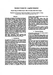
Results for an ensemble of 100 random trees is shown in Table 4. We can see that GPU Random Forests clearly outperforms MOA for all three datasets, being up to 1300x faster than MOA for the RT dataset. Table 4: Comparison of the speed of MOA Random Forest vs GPU

Random Forest. Cov REC RT

MOA 363s 1 778s 795s

GPU RF 0.330s 5.740s 0.597s

Speedup 1000x 309x 1300x

In this test, 100 random trees run on the GPU at the same time, thus generating more threads for the GPU to schedule. The higher the number of threads available to run contemporarily on the GPU, the better its latency gets hidden. Compared to a single GVFDT tree, ensembles are 2–5 times slower, but obtain higher accuracy. Figure 11 shows how MOA and GPU Random Forests scale with the number of instances of the REC dataset. In this dataset MOA scales linearly while GPU Random Forests seems to scale almost constantly. This is an effect of the scale, as GPU Random Forests runs in milliseconds instead of minutes. In summary, we can appreciate that GPU Random Forests performs much better than MOA Random Forests for all three datasets.

7

CONCLUSIONS

In this paper we presented efficient streaming Very Fast Decision Trees and Random Forests algorithms designed for the GPU. We started by identifying the phases of execution of the decision tree algorithm, extended them horizontally to increase parallelism, and studied how each of them could be implemented on the GPU. Our streaming Random Forest algorithm uses a per-tree adaptive mechanism to detect changes on the stream so it can react to it. These new methods minimize the communication between the GPU and the CPU to the point that they only need to communicate when the

CPU has new instances to process and when the GPU sends the results back to the CPU. We showed how using our adaptive streaming Random Forest on GPUs, speed increases at least 300x. This huge improvement in speed using GPUs opens new exciting possibilities for future research on streaming machine learning.

REFERENCES [1] Albert Bifet and Ricard Gavald`a, ‘Learning from timechanging data with adaptive windowing’, in In SIAM International Conference on Data Mining, (2007). [2] Albert Bifet, Geoff Holmes, Richard Kirkby, and Bernhard Pfahringer, ‘MOA: Massive Online Analysis’, Journal of Machine Learning Research (JMLR), (2010). [3] Leo Breiman, ‘Random forests’, Machine Learning, 45(1), 5– 32, (2001). [4] Adam Coates, Brody Huval, Tao Wang, David J. Wu, Bryan C. Catanzaro, and Andrew Y. Ng, ‘Deep learning with cots hpc systems’, in ICML (3), pp. 1337–1345, (2013). [5] Pedro Domingos and Geoff Hulten, ‘Mining high-speed data streams’, in ACM SIGKDD, KDD ’00, pp. 71–80, (2000). [6] Tim Foley and Jeremy Sugerman, ‘KD-tree Acceleration Structures for a GPU Raytracer’, HWWS ’05, pp. 15–22, (2005). [7] Michael Goldfarb, Youngjoon Jo, and Milind Kulkarni, ‘General Transformations for GPU Execution of Tree Traversals’, SC ’13, pp. 10:1–10:12, (2013). [8] Hakan Grahn, Niklas Lavesson, Mikael Hellborg Lapajne, and Daniel Slat, ‘CudaRF: A CUDA-based Implementation of Random Forests’, AICCSA ’11, pp. 95–101, (2011). [9] Daniel Reiter Horn, Jeremy Sugerman, Mike Houston, and Pat Hanrahan, ‘Interactive K-d Tree GPU Raytracing’, I3D ’07, pp. 167–174, New York, NY, USA, (2007). ACM. [10] Geoff Hulten and Pedro Domingos. VFML – a toolkit for mining high-speed time-changing data streams, 2003. [11] G. Jacobson, ‘Space-efficient static trees and graphs’, SFCS ’89, pp. 549–554, (1989). [12] Tero Karras, ‘Maximizing Parallelism in the Construction of BVHs, Octrees, and K-d Trees’, in ACM SIGGRAPH, EGGHHPG’12, pp. 33–37, (2012). [13] Yisheng Liao. CudaTree, a python library, 2013. [14] Nikunj C. Oza and Stuart Russell, ‘Experimental comparisons of online and batch versions of bagging and boosting’, in KDD ’01, pp. 359–364, (2001). [15] Stefan Popov, Johannes G¨unther, Hans-Peter Seidel, and Philipp Slusallek, ‘Stackless KD-Tree Traversal for High Performance GPU Ray Tracing’, volume 26, pp. 415–424, (2007).